Novel Numerical Approach Based on Modified Extended Cubic B-Spline Functions for Solving Non-Linear Time-Fractional Telegraph Equation

Abstract

The telegraph model describes that the current and voltage waves can be reflected on a wire, that symmetrical wave patterns can form along a line. A numerical study of these voltage and current waves on a transferral line has been proposed via a modified extended cubic B-spline (MECBS) method. The B-spline functions have the flexibility and high order accuracy to approximate the solutions. These functions also preserve the symmetrical property. The MECBS and Crank Nicolson technique are employed to find out the solution of the non-linear time fractional telegraph equation. The time direction is discretized in the Caputo sense while the space dimension is discretized by the modified extended cubic B-spline. The non-linearity in the equation is linearized by Taylor’s series. The proposed algorithm is unconditionally stable and convergent. The numerical examples are displayed to verify the authenticity and implementation of the method.

1. Introduction

Transmission line equation is the other name known for the classical telegraph equation (TE) due to the reason of its origination because of the connection amongst voltage and the current waves on the transferral line. The common diffusion circumstance is explained well such an equation. However, in case of finite long transmits procedure, when the situation of abnormal diffusion happens (in presence of voltage wave or current wave), the classical TE does not completely explain well. FTE works well in such type of scenarios. Cascaval et al. [1] analysed FTE happens to facilitate in improved understanding of diffusion process present in blood flow investigations. The FTE has been used into the modeling of reaction dissemination, signal analysis for transference, random walk of suspension flow, propagation of electrical signals etc.

Consider the nonlinear time fractional telegraph equation (FTE) [2]

$$\frac{{\partial }^{2\alpha }u(s,t)}{\partial t^{2\alpha }}+\gamma \frac{{\partial }^{\alpha }u(s,t)}{\partial t^{\alpha }}-\frac{{\partial }^{2}u(s,t)}{\partial s^2}+\psi \left(u(s,t)\right)=g(s,t),s\in \mathsf{\Omega },t\ge 0,$$

(1)

with initial conditions

$$\left\{\begin{array}{c}u(s,0)={\varphi }_1\left(s\right),s\in \mathsf{\Omega }\hfill \\ u_t(s,0)={\varphi }_2\left(s\right),s\in \mathsf{\Omega }\hfill \\ u(s,t)=g_1\left(t\right),t\ge 0\hfill \\ u(s,t)=g_2\left(t\right),\hfill \end{array}\right.$$

(2)

where $\gamma >0$, g are a constant and suitable prescribed function of s and t respectively. $\psi \left(u(s,t)\right)={\gamma }_1{u}^3(s,t)+{\gamma }_2{u}^2(s,t)+{\gamma }_{3}u(s,t),$${\gamma }_1,$${\gamma }_2,$${\gamma }_3,$ are real constants. $\alpha$, $\mathsf{\Omega }$ denote fractional derivative and bounded domain in real functions. Furthermore, $\frac{{\partial }^{2\alpha }u(s,t)}{\partial t^{2\alpha }}$, $\frac{{\partial }^{\alpha }u(s,t)}{\partial t^{\alpha }}$ are Caputo fractional derivatives (CFD) and $\alpha \in (0,1)$. The CFD [3] is interpreted as follows:

$$D_C^{\alpha }F\left(x\right)=\left\{\begin{array}{cc}\frac{1}{\mathsf{\Gamma }(n-\alpha )}{\int }_0^x{(x-\xi )}^{n-1-\alpha }{F}^{\left(n\right)}\left(\xi \right)d\xi ,\hfill & n-1<\alpha \le n,n\in N,\hfill \\ F^{\left(n\right)}\left(x\right),\hfill & \alpha =n.\hfill \end{array}\right.$$

(3)

where $\mathsf{\Gamma }$ is the Euler’s Gamma function. The CFD allows traditional initial and boundary conditions to be involved in the formula of the modeled problem. Here, the CFD of a constant equals to zero [4,5].

Several numerical and analytical techniques have been developed to solve FTE. The Adomian decomposition method has been proposed for the analytical solution of FTE by Momani [6]. In this article fractional derivatives have been used in Caputo sence. Yildirim [7] investigated He’s homotopy technique for the solution of space-time FTE. The analytical solution has been calculated in the form of series solutions. Das et al. [8] presented an analytical solution of time FTE using homotopy analysis method. A linear time FTE has been solved by Li and Cao [9] via finite difference (FD) algorithm. Galerkin mixed finite element technique for the solution of time FTE has been proposed by Wang [10]. A combination of Sumudu variational and iteration technique for solving FTE has been proposed by Alkahtani et al. [11]. Asgari et al. [12] solved time FTE using Bernstein ploynomials operational matrices. A combined method of a group preserving technique and the technique of line with CFD has been proposed by Hashemi and Baleanu [13]. A collocation technique based on radial basis function for the numerical solution of nonlinear time FTE has been proposed by Sepehrian and Shamohammadi [2]. Wang et al. [14] discussed the reproducing kernel space algorithm with CFD for solving time FTE numerically. Wang and Mei [15] presented a Legendre spectral Galerkin technique and generalized FD technique for solving time FTE. Liu [16] presented difference approximations for solving time FTE via Grünwald formula and CFD.

B-splines functions have adaptability to estimate the solution with high order precision at any point in the domain. These basis functions have been used to obtain the solution of fractional differential equations (FDEs). Several researchers have been utilized B-splines to obtain the solution of FDEs but only short number of studies for the FTE. Furthermore, so far as we realise there is no such research on the use of B-spline for solving non-linear telegraph equation. Esen and Tasbozan [17] solved the fractional Burgers equation using quadratic B-spline Galerkin approach. Sayevand et al. [18] discussed a numerical technique for fractional diffusion problems via cubic B-spline (CBS). Pitolli [19] presented the solutions of the Predator-Prey models using fractional B-spline technique. The FD algorithm via extended cubic B-spline (ECBS) has been proposed for the time fractional advection diffusion model by Mohyud-Din et al. [20]. Ghalomian and Nadjafi [21] presented the solution of integro-differential model using CBS approach. Akram et al. [22,23,24] developed numerical techniques for the linear time fractional telegraph model and fractional diffusion models via ECBS functions and CFD. Khalid et al. [25] discussed time fractional Allen–Cahn model using redefine CBS functions.

The collocation method with B-splines functions is shown to provide good results for FDEs. The main advantage of this method is that the obtained solution will be in approximate analytical form. Then the numerical solution can be established from the approximate analytical solution at any discrete point.

This paper is organised as follows: In Section 2, a modified basis function is introduced. In Section 3, a MECBS, Crank–Nicolson method and Caputo’s derivative are applied to solve nonlinear FTE. Section 4 and Section 5 are devoted to stability analysis and convergence analysis. In Section 6, numerical examples are illustrated. Finally conclusion is demonstrated in Section 7.

2. Modified Basis Function

Consider $\left\{s_i\right\}$ be a equally spaced partitioning of a finite domain with $i\in \mathbb{Z}$. Therefore, supposed interval is arranged into M equal subintervals at the nodes as $s_i=s_0+ih$, where h is a step size. The ECBS functions [26] at the $s_i$ over the assumed interval is presented as follows;

$$E_i(s,\eta )=\frac{1}{24h^4}\left\{\begin{array}{cc}4h(1-\eta ){(s-s_{i-2})}^3+3\eta {(s-s_{i-2})}^4,\hfill & s\in [s_{i-2},s_{i-1}),\hfill \\ (4-\eta )h^4+12h^3(s-s_{i-1})+6h^2(2+\eta ){(s-s_{i-1})}^2\hfill \\ -12h{(s-s_{i-1})}^3-3\eta {(s-s_{i-1})}^4,\hfill & s\in [s_{i-1},s_i),\hfill \\ (4-\eta )h^4+12h^3(s_{i+1}-s)+6h^2(2+\eta ){(s_{i+1}-s)}^2\hfill \\ -12h{(s_{i+1}-s)}^3-3\eta {(s_{i+1}-s)}^4,\hfill & s\in [s_i,s_{i+1}),\hfill \\ 4h(1-\eta ){(s_{i+2}-s)}^3+3\eta {(s_{i+2}-s)}^4,\hfill & s\in [s_{i+1},s_{i+2}),\hfill \\ 0,\hfill & \mathrm{otherwise}.\hfill \end{array}\right.$$

(4)

where $i=-1\left(1\right)M+1$, $\eta \in \mathbb{R}$ is a free parameter in the closed interval $[-8,1]$ and $s\in \mathbb{R}$ is a variable. For $\eta \in [-8,1]$, the CBS and ECBS basis hold same properties such as convex hull, symmetry, geometrical invariability. The CBS and ECBS basis functions are numerically stable due to the convex hull and symmetry properties. The ECBS transforms into CBS for $\eta =0$. For a smooth function $u(s,t)$ there is a unique $U(s,t)$, that assures the determined conditions, such that

$$U(s,t)=\sum _{i=j-1}^{j+1}{d}_i^n\left(t\right)E_i(s,\eta ),$$

(5)

where time dependent unknown coefficients $d_j\left(t\right)$’s are carried out by some specific restrictions. The ECBS functions (4) and Equation (5) produce the following relations

$$U_j(s,t)=\sum _{i=j-1}^{j+1}{d}_i\left(t\right)E_i(s,\eta )=\left(\frac{4-\eta }{24}\right)d_{j-1}+\left(\frac{8+\eta }{12}\right)d_j+\left(\frac{4-\eta }{24}\right)d_{j+1}$$

(6)

$$U_j^{\prime }(s,t)=\sum _{i=j-1}^{j+1}{d}_i\left(t\right)E_i^{\prime }(s,\eta )=\left(-\frac{1}{2h}\right)d_{j-1}+\left(\frac{1}{2h}\right)d_{j+1}$$

(7)

$$U_j^{″}(s,t)=\sum _{i=j-1}^{j+1}{d}_i\left(t\right)E_i^{″}(s,\eta )=\left(\frac{2+\eta }{2h^2}\right)d_{j-1}+\left(-\frac{4+2\eta }{2h^2}\right)d_j+\left(\frac{2+\eta }{2h^2}\right)d_{j+1}.$$

(8)

In this article, the modified basis function are defined as follows

$$\left\{\begin{array}{cc}\widetilde{E_0}\left(s\right)=E_0\left(s\right)+2E_{-1}\left(s\right),\hfill & \mathrm{for}j=0\hfill \\ \widetilde{E_1}\left(s\right)=E_1\left(s\right)-E_{-1}\left(s\right),\hfill & \mathrm{for}j=1\hfill \\ \widetilde{E_j}\left(s\right)=E_j\left(s\right),\hfill & \mathrm{for}j=2,\dots ,M-2\hfill \\ {\tilde{E}}_{M-1}\left(s\right)=E_{M-1}\left(s\right)-E_{M+1}\left(s\right),\hfill & \mathrm{for}j=M-1\hfill \\ {\tilde{E}}_M\left(s\right)=E_M\left(s\right)+2E_{M+1}\left(s\right),\hfill & \mathrm{for}j=M.\hfill \end{array}\right.$$

(9)

The ECBS functions are modified in this way that the diagonally dominance property is hold [27]. Now approximated solution of modified basis is described as follows

$$\left\{\begin{array}{cc}U(s_0,t)=g_1\left(t\right),\hfill & \mathrm{for}j=0\hfill \\ U(s_j,t)=\sum _{j=0}^M{d}_j\widetilde{E_j}\left(s\right),\hfill & \mathrm{for}j=1,\dots ,M-1\hfill \\ U(s_M,t)=g_2\left(t\right),\hfill & \mathrm{for}j=M.\hfill \end{array}\right.$$

(10)

3. Derivation of the Method

In this part, we develop the numerical technique to solve the nonlinear time FTE using CFD. Take uniform partition of time interval as $t_m=t_0+m\tau$ with $\tau =t_{m+1}-t_m$, $m=0,1,\dots ,N-1$. The discretization of $\frac{{\partial }^{2\alpha }u(s,t)}{\partial t^{2\alpha }}$ and $\frac{{\partial }^{\alpha }u(s,t)}{\partial t^{\alpha }}$ in CFD form [28] are described as follows

$$\begin{array}{cc}& \frac{{\partial }^{2\alpha }u(s,t_{m+1})}{\partial t^{2\alpha }}\hfill \\ =& \frac{1}{\mathsf{\Gamma }(2-2\alpha )}{\int }_0^t\frac{{\partial }^{2}u(s,\sigma )}{\partial {\sigma }^2}\frac{d\sigma }{{(t_{m+1}-\sigma )}^{2\alpha -1}}\hfill \\ =& \frac{1}{\mathsf{\Gamma }(2-2\alpha )}\sum _{p=0}^m{\int }_{t_p}^{t_{p+1}}\frac{{\partial }^{2}u(s,\sigma )}{\partial {\sigma }^2}\frac{d\sigma }{{(t_{m+1}-\sigma )}^{2\alpha -1}}\hfill \\ =& \frac{1}{\mathsf{\Gamma }(2-2\alpha )}\sum _{p=0}^m\frac{u(s,t_{p+1})-2u(s,t_p)+u(s,t_{p-1})}{{\tau }^2}{\int }_{t_p}^{t_{p+1}}\frac{d\sigma }{{(t_{m+1}-s)}^{2\alpha -1}}+e_{\tau }^{m+1}\hfill \end{array}$$

$$\frac{{\partial }^{2\alpha }u(s,t^{m+1})}{\partial t^{2\alpha }}=\frac{1}{\mathsf{\Gamma }(3-2\alpha )}\sum _{p=0}^m{b}_p^{\ast }\frac{u(s,t^{m-p+1})-2u(s,t^{m-p})+u(s,t^{m-p-1})}{{\tau }^{2\alpha }}+e_{\tau }^{m+1},$$

(11)

where $b_p^{\ast }={(p+1)}^{2-2\alpha }-p^{2-2\alpha }$. The truncation error $e_{\tau }^{m+1}$ is given in [29] as

$$\begin{array}{c}\hfill |e_{\tau }^{m+1}|\le C{\tau }^{3-2\alpha },\end{array}$$

(12)

Remark 1.

For $\alpha \in (0,0.5)$, the given telegraph model becomes first order in time direction. Therefore always $\alpha \in (0.5,1)$.

And

$$\begin{array}{ccc}\hfill \frac{{\partial }^{\alpha }u(s,t_{m+1})}{\partial t^{\alpha }}& =& \frac{1}{\mathsf{\Gamma }(1-\alpha )}{\int }_0^t\frac{\partial u(s,\sigma )}{\partial \sigma }\frac{d\sigma }{{(t_{m+1}-\sigma )}^{\alpha }},\hfill \\ & =& \frac{1}{\mathsf{\Gamma }(1-\alpha )}\sum _{p=0}^m{\int }_{t_p}^{t_{p+1}}\frac{\partial u(s,\sigma )}{\partial \sigma }\frac{d\sigma }{{(t_{m+1}-\sigma )}^{\alpha }},\hfill \\ & =& \frac{1}{\mathsf{\Gamma }(1-\alpha )}\sum _{p=0}^m\frac{u(s,t_{p+1})-u(s,t_p)}{\tau }{\int }_{t_p}^{t_{p+1}}\frac{d\sigma }{{(t_{m+1}-\sigma )}^{\alpha }}+e_1^{m+1},\hfill \\ & =& \frac{1}{\mathsf{\Gamma }(2-\alpha )}\sum _{p=0}^m\frac{u(s,t_{m-p+1})-u(s,t_{m-p})}{{\tau }^{\alpha }}\left({(p+1)}^{1-\alpha }-p^{1-\alpha }\right)+e_1^{m+1},\hfill \end{array}$$

$$\begin{array}{c}\hfill \frac{{\partial }^{\alpha }u(s,t^{m+1})}{\partial t^{\alpha }}=\frac{1}{\mathsf{\Gamma }(2-\alpha )}\sum _{p=0}^m{b}_p\frac{u(s,t^{m-p+1})-u(s,t^{m-p})}{{\tau }^{\alpha }}+e_1^{m+1},\end{array}$$

(13)

where $b_p={(p+1)}^{1-\alpha }-p^{1-\alpha }$. The truncation error of first order $e_1^{m+1}$ is defined in [30] as

$$\begin{array}{c}\hfill |e_1^{m+1}|\le C_1{\tau }^{2-\alpha },\end{array}$$

(14)

where C and $C_1$ are constants.

The $b_p$, $b_p^{\ast }$ satisfy the following conditions

$$\left\{\begin{array}{c}{b}_0=1\hfill \\ b_0>b_1>b_2>\dots >b_p,b_p\to 0asp\to \infty \hfill \\ b_p>0forp=0,1,\dots ,m\hfill \\ \sum _{p=0}^m(b_p-b_{p+1})+b_{m+1}=(1-b_1)+\sum _{p=1}^{m-1}(b_p-b_{p+1})+b_m=1\hfill \\ \sum _{p=2}^{m-1}(2b_p^{\ast }-b_{p-1}^{\ast })+b_{p-1}^{\ast },\forall p=1,2,\dots ,m.\hfill \end{array}\right.$$

Using $\theta$ weighted technique and Equations (11) and (13) in Equation (1), we obtain

$$\begin{array}{c}\frac{{\tau }^{-2\alpha }}{\mathsf{\Gamma }(3-2\alpha )}\sum _{p=0}^m{b}_p^{\ast }[u^{m-p+1}-2u^{m-p}+u^{m-p-1}]+\frac{\gamma {\tau }^{-\alpha }}{\mathsf{\Gamma }(2-\alpha )}\sum _{p=0}^m{b}_p[u^{m-p+1}-u^{m-p}]\hfill \\ \hfill +\theta (-u_{ss}^{m+1}+\psi \left(u^{m+1}\right))+(1-\theta )(-u_{ss}^m+\psi \left(u^m\right))=g^{m+1},\end{array}$$

(15)

It is perceived that the $u^{-1}$ will arise for $j=0,m$, where $m=0,1,\dots ,N$. The central difference formula is used to obtain this term:

$$u^{-1}=u^1-2\tau {\varphi }_2\left(s\right).$$

Nonlinear term is linearized [31] as follow

$${\left(u^2\right)}^{m+1}=2u^m{u}^{m+1}-u^m{u}^m+O{\left(\tau \right)}^2$$

(16)

$${\left(u^3\right)}^{m+1}=3{\left(u^2\right)}^m{u}^{m+1}-2{\left(u^3\right)}^m+O{\left(\tau \right)}^2$$

(17)

here, if we choose $\theta =0,$$\frac{1}{2}$ and 1, the above equation gives explicit, Crank–Nicolson and implicit method. Substituting $\theta =\frac{1}{2}$ in (15), we obtain Crank–Nicolson scheme as follows:

$$\begin{array}{c}{r}_1\sum _{p=0}^m{b}_p^{\ast }[u^{m-p+1}-2u^{m-p}+u^{m-p-1}]+r_2\sum _{p=0}^m{b}_p[u^{m-p+1}-u^{m-p}]\hfill \\ -\frac{1}{2}(u_{ss}^{m+1}+u_{ss}^m)+\frac{{\gamma }_1}{2}\left({\left(u^3\right)}^{m+1}+{\left(u^3\right)}^m\right)+\frac{{\gamma }_2}{2}\left({\left(u^2\right)}^{m+1}+{\left(u^2\right)}^m\right)\\ \hfill +\frac{{\gamma }_3}{2}\left(u^{m+1}+u^m\right)=g^{m+1},\end{array}$$

(18)

where $r_1=\frac{{\tau }^{-2\alpha }}{\mathsf{\Gamma }(3-2\alpha )},$$r_2=\frac{\gamma {\tau }^{-\alpha }}{\mathsf{\Gamma }(2-\alpha )}$. Using (16), (17) in (18), we have

$$\begin{array}{c}(r_1+r_2+\frac{{\gamma }_3}{2})u^{m+1}-\frac{u_{ss}^{m+1}}{2}+{\gamma }_2{u}^m{u}^{m+1}+\frac{3{\gamma }_1}{2}{\left(u^2\right)}^m{u}^{m+1}\hfill \\ =(2r_1+r_2-\frac{{\gamma }_3}{2})u^m-r_1{u}^{m-1}+\frac{u_{ss}^m}{2}+\frac{{\gamma }_1}{2}{\left(u^3\right)}^m-r_1\sum _{p=1}^m{b}_p^{\ast }[u^{m-p+1}\\ \hfill -2u^{m-p}+u^{m-p-1}]-r_2\sum _{p=1}^m{b}_p[u^{m-p+1}-u^{m-p}]+g^{m+1}\end{array}$$

Using (10) in the above equation, for $j=0,1,\dots ,M,$ we have

$$\begin{array}{c}(r_1+r_2+\frac{{\gamma }_3}{2})\sum _{j=0}^M{d}_j^{m+1}{\tilde{E}}_j\left(s\right)-\frac{1}{2}\sum _{j=0}^M{d}_j^{m+1}{\tilde{E}}_j^{″}\left(s\right)+{\gamma }_2\sum _{j=0}^M{d}_j^m{\tilde{E}}_j\left(s\right)\sum _{j=0}^M{d}_j^{m+1}{\tilde{E}}_j\left(s\right)\hfill \\ +\frac{3{\gamma }_1}{2}\sum _{j=0}^M{d}_j^m{\tilde{E}}_j^2\left(s\right)\sum _{j=0}^M{d}_j^{m+1}{\tilde{E}}_j\left(s\right)=(2r_1+r_2-\frac{{\gamma }_3}{2})\sum _{j=0}^M{d}_j^m{\tilde{E}}_j\left(s\right)-r_1\sum _{j=0}^M{d}_j^{m-1}{\tilde{E}}_j\left(s\right)\\ +\frac{1}{2}\sum _{j=0}^M{d}_j^m{\tilde{E}}_j^{″}\left(s\right)+\frac{{\gamma }_1}{2}\sum _{j=0}^M{d}_j^m{\tilde{E}}_j^3\left(s\right)-r_1\sum _{p=1}^m{b}_p^{\ast }[\sum _{j=0}^M{d}_j^{m-p+1}{\tilde{E}}_j\left(s\right)-2\sum _{j=0}^M{d}_j^{m-p}{\tilde{E}}_j\left(s\right)\\ \hfill +\sum _{j=0}^M{d}_j^{m-p-1}{\tilde{E}}_j\left(s\right)]-r_2\sum _{p=1}^m{b}_p\left[\sum _{j=0}^M{d}_j^{m-p+1}{\tilde{E}}_j\left(s\right)-\sum _{j=0}^M{d}_j^{m-p}{\tilde{E}}_j\left(s\right)\right]+g^{m+1}.\end{array}$$

The above system have $(M+1)\times (M+1)$, we can solve it uniquely. In order to begin the iteration on the above system, it is mandatory to obtain the initial vector, for this we will utilize initial conditions

$$\left\{\begin{array}{cc}{\tilde{E}}_0^{m+1}={\varphi }_1^0\left(s_j\right),\hfill & j=0,\hfill \\ \sum _{j=0}^M{d}_j^{m+1}{\tilde{E}}_j={\varphi }_1^0\left(s_j\right),\hfill & j=1,\dots ,M-1,\hfill \\ {\tilde{E}}_M^{m+1}={\varphi }_1^0\left(s_j\right),\hfill & j=M.\hfill \end{array}\right.$$

(19)

The above system (19) can be written as

$$A{d}^0=B$$

where

$$A=\frac{1}{24}\left[\begin{array}{ccccccc}24& 0& 0& 0& \dots & \dots & 0\\ 4-\eta & 2(8+\eta )& 4-\eta & 0& \dots & \dots & 0\\ 0& 4-\eta & 2(8+\eta )& 4-\eta & \dots & \dots & 0\\ ⋮& \dots & \ddots & \ddots & \ddots & \dots & ⋮\\ ⋮& \dots & \dots & \dots & 4-\eta & 2(8+\eta )& 4-\eta \\ 0& \dots & \dots & \dots & 0& 0& 24\end{array}\right]$$

$B={[g_1\left(s_0\right),\dots ,g_1\left(s_M\right)]}^T$. It is clearly observed that for $\eta >-2$ the matrix A is strictly diagonally dominant. Therefore invertible by Gershgorin’s theorem [32]. Therefore, the above system cab be solved easily by Wolfram Mathematica 12.

4. Stability Analysis

The idea of stability is related to the errors of computational method do not grow as the execution continues. We will employ Von Neumann technique to examine the stability analysis. Let ${\mathsf{{\rm Y}}}^m$ represents the growth factor in the form of Fourier mode and suppose ${\mathsf{{\rm Y}}}^{\ast m}$ be the computed value. Therefore the error ${\xi }^m$ at mth time level is defined as

$${\xi }^m={\mathsf{{\rm Y}}}^m-{\mathsf{{\rm Y}}}^{\ast m}.$$

Consider the linearization [31] of (18) as $\psi \left(u\right)=({\gamma }_1{u}^2+{\gamma }_{2}u+{\gamma }_3)u=\lambda u$, we have the following error equation:

$$\begin{array}{c}(r_1+r_2+\frac{\lambda }{2}){\xi }^{m+1}-\frac{{\xi }_{ss}^{m+1}}{2}=(2r_1+r_2-\frac{\lambda }{2}){\xi }^m-r_1{\xi }^{m-1}+\frac{{\xi }_{ss}^{m+1}}{2}\hfill \\ \hfill -r_1\sum _{p=0}^m{b}_p^{\ast }[{\xi }^{m+1-p}-2{\xi }^{m-p}+{\xi }^{m-p-1}]-r_2\sum _{p=0}^m{b}_p[{\xi }^{m+1-p}-{\xi }^{m-p}].\end{array}$$

(20)

Suppose the modified basis difference equation in one Fourier mode as

$${\xi }_j^{m+1}={\delta }^m{e}^{i\beta hj},$$

where $i=\sqrt{-1}$, $\beta$, $\delta$, h are the mode number, the Fourier coefficient and the element size respectively, then the expression (20) takes the form

$$\begin{array}{c}(r_1+r_2+\frac{\lambda }{2}){\xi }^{m+1}-\frac{{\xi }_{ss}^{m+1}}{2}=(2r_1+r_2-\frac{\lambda }{2}){\xi }^m-r_1{\xi }^{m-1}+\frac{{\xi }_{ss}^{m+1}}{2}\hfill \\ \hfill -r_1\sum _{p=0}^m{b}_p^{\ast }[{\xi }^{m+1-p}-2{\xi }^{m-p}+{\xi }^{m-p-1}]-r_2\sum _{p=0}^m{b}_p[{\xi }^{m+1-p}-{\xi }^{m-p}],\end{array}$$

(21)

Using the basis function, Equation (21) reduces to

$$\begin{array}{c}[(r_1+r_2+\frac{\lambda }{2})\left(\left(\frac{4-\eta }{24}\right)e^{i\beta h(j-1)}+\left(\frac{8+\eta }{12}\right)e^{i\beta hj}+\left(\frac{4-\eta }{24}\right)e^{i\beta h(j+1)}\right)\hfill \\ -\frac{1}{2}\left(\left(\frac{2+\eta }{2h^2}\right)e^{i\beta h(j-1)}+\left(-\frac{2+\eta }{h^2}\right)e^{i\beta hj}+\left(\frac{2+\eta }{h^2}\right)e^{i\beta h(j+1)}\right)]{\delta }^{m+1}=\\ (2r_1+r_2-\frac{\lambda }{2})\left[\left(\frac{4-\eta }{24}\right)e^{i\beta h(j-1)}+\left(\frac{8+\eta }{12}\right)e^{i\beta hj}+\left(\frac{4-\eta }{24}\right)e^{i\beta h(j+1)}\right]{\delta }^m\\ -r_1\left[\left(\frac{4-\eta }{24}\right)e^{i\beta h(j-1)}+\left(\frac{8+\eta }{12}\right)e^{i\beta hj}+\left(\frac{4-\eta }{24}\right)e^{i\beta h(j+1)}\right]{\delta }^{m-1}\\ +\frac{1}{2}\left[\left(\frac{2+\eta }{2h^2}\right)e^{i\beta h(j-1)}+\left(-\frac{2+\eta }{h^2}\right)e^{i\beta hj}+\left(\frac{2+\eta }{h^2}\right)e^{i\beta h(j+1)}\right]-r_1\sum _{p=0}^m{b}_p^{\ast }[{\delta }^{m+1-p}\\ -2{\delta }^{m-p}+{\delta }^{m-p-1}]\left[\left(\frac{4-\eta }{24}\right)e^{i\beta h(j-1)}+\left(\frac{8+\eta }{12}\right)e^{i\beta hj}+\left(\frac{4-\eta }{24}\right)e^{i\beta h(j+1)}\right]\\ \hfill -r_2\sum _{p=0}^m{b}_p[{\delta }^{m+1-p}-{\delta }^{m-p}]\left[\left(\frac{4-\eta }{24}\right)e^{i\beta h(j-1)}+\left(\frac{8+\eta }{12}\right)e^{i\beta hj}+\left(\frac{4-\eta }{24}\right)e^{i\beta h(j+1)}\right],\end{array}$$

(22)

Divide (22) by $e^{i\beta hj}$ and incorporating the terms, we attain

$$\begin{array}{c}\left[(r_1+r_2+\frac{\lambda }{2})\left(\frac{8+\eta }{12}+2\frac{4-\eta }{24}cos\left(\beta h\right)\right)-\frac{1}{2}\left(-\frac{2+\eta }{h^2}+2\frac{2+\eta }{2h^2}cos\left(\beta h\right)\right)\right]{\delta }^{m+1}=\hfill \\ \left[(2r_1+r_2-\frac{\lambda }{2})\left(\frac{8+\eta }{12}+2\frac{4-\eta }{24}cos\left(\beta h\right)\right)+\frac{1}{2}\left(-\frac{2+\eta }{h^2}+2\frac{2+\eta }{2h^2}cos\left(\beta h\right)\right)\right]{\delta }^m\\ -r_1\left[\frac{8+\eta }{12}+2\frac{4-\eta }{24}cos\left(\beta h\right)\right]{\delta }^{m-1}-r_1\left(\frac{8+\eta }{12}+2\frac{4-\eta }{24}cos\left(\beta h\right)\right)\sum _{p=0}^m{b}_p^{\ast }[{\delta }^{m+1-p}\\ \hfill -2{\delta }^{m-p}+{\delta }^{m-p-1}]-r_2\left(\frac{8+\eta }{12}+2\frac{4-\eta }{24}cos\left(\beta h\right)\right)\sum _{p=0}^m{b}_p[{\delta }^{m+1-p}-{\delta }^{m-p}]\end{array}$$

Throughout divide by $\frac{8+\eta }{12}+2\frac{4-\eta }{24}cos\left(\beta h\right)$, we achieve

$$\begin{array}{c}[(r_1+r_2+\frac{\lambda }{2})+v]{\delta }^{m+1}=[(2r_1+r_2-\frac{\lambda }{2})-v]{\delta }^m-r_1{\delta }^{m-1}\hfill \\ \hfill -r_1\sum _{p=0}^m{b}_p^{\ast }[{\delta }^{m+1-p}-2{\delta }^{m-p}+{\delta }^{m-p-1}]-r_2\sum _{p=0}^m{b}_p[{\delta }^{m+1-p}-{\delta }^{m-p}],\end{array}$$

(23)

where $v=\frac{(2+\eta ){sin}^2\beta h/2}{h^2(6+(\eta -4){sin}^2\beta h/2)}\ge 0$ for all $\eta >-2$.

Proposition 1.

If ${\delta }^m,m=0,1,\dots ,N$ be the solution of (23), then $|{\delta }^k|\le |{\delta }^0|$.

Proof. 

We determine this results by mathematical induction. Using $m=0$ in expression (23), we get

$$\begin{array}{ccc}\hfill (r_1+r_2+\frac{\lambda }{2}+v){\delta }^1& =& (2r_1+r_2-\frac{\lambda }{2}-v){\delta }^0-r_1{\delta }^{-1}\hfill \\ \hfill (r_1+r_2+\frac{\lambda }{2}+v){\delta }^1& =& (2r_1+r_2-\frac{\lambda }{2}-v){\delta }^0\hfill \\ \hfill {\delta }^1& =& \left[\frac{2r_1+r_2-\frac{\lambda }{2}-v}{2r_1+r_2+\frac{\lambda }{2}+v}\right]{\delta }^0\hfill \\ \hfill |{\delta }^1|& \le & |{\delta }^0|.\hfill \end{array}$$

Suppose that for $m=0,1,\dots ,N-1$, $|{\delta }^m|\le |{\delta }^0|$ is true then we have

$$\begin{array}{ccc}\hfill (r_1+r_2+\frac{\lambda }{2}+v){\delta }^{m+1}& =& (2r_1+r_2-\frac{\lambda }{2}-v){\delta }^m-r_1{\delta }^{m-1}-r_1\sum _{p=0}^m{b}_p^{\ast }[{\delta }^{m+1-p}\hfill \\ & -& 2{\delta }^{m-p}+{\delta }^{m-p-1}]-r_2\sum _{p=0}^m{b}_p[{\delta }^{m+1-p}-{\delta }^{m-p}]\hfill \\ \hfill (r_1+r_2+\frac{\lambda }{2}+v){\delta }^{m+1}& \le & (2r_1+r_2){\delta }^m-r_1{\delta }^{m-1}-r_1\sum _{p=0}^m{b}_p^{\ast }[{\delta }^{m+1-p}-2{\delta }^{m-p}\hfill \\ & +& {\delta }^{m-p-1}]-r_2\sum _{p=0}^m{b}_p[{\delta }^{m+1-p}-{\delta }^{m-p}]\hfill \\ \hfill (r_1+r_2+\frac{\lambda }{2}+v)|{\delta }^{m+1}|& \le & |(2r_1+r_2){\delta }^m-r_1{\delta }^{m-1}|+r_1\sum _{p=0}^m{b}_p^{\ast }\left[\right|{\delta }^{m+1-p}\hfill \\ & -& 2{\delta }^{m-p}+{\delta }^{m-p-1}\left|\right]+r_2\sum _{p=0}^m{b}_p\left[\right|{\delta }^{m+1-p}-{\delta }^{m-p}\left|\right]\hfill \end{array}$$

$$\begin{array}{ccc}& =& |(2r_1+r_2){\delta }^m-r_1{\delta }^{m-1}|+r_1\sum _{p=0}^m{b}_p^{\ast }\left[\right|{\delta }^{m+1-p}-{\delta }^{m-p}|\hfill \\ & +& |{\delta }^{m-p-1}-{\delta }^{m-p}\left|\right]+r_2\sum _{p=0}^m{b}_p\left[\right|{\delta }^{m+1-p}-{\delta }^{m-p}\left|\right]\hfill \\ & =& |(2r_1+r_2)|{\delta }^m|-r_1|{\delta }^{m-1}\left|\right|+r_1\sum _{p=0}^m{b}_p^{\ast }\left[\right||{\delta }^{m+1-p}|\hfill \\ & -& |{\delta }^{m-p}\left|\right|+\left|\right|{\delta }^{m-p-1}|-|{\delta }^{m-p}\left|\right|]+r_2\sum _{p=0}^m{b}_p\left[\right||{\delta }^{m+1-p}|\hfill \\ & -& |{\delta }^{m-p}\left|\right|]\hfill \\ \hfill (r_1+r_2+\frac{\lambda }{2}+v)\left|{\delta }^{m+1}\right|& \le & |(2r_1+r_2)|{\delta }^0|-r_1|{\delta }^0\left|\right|+r_1\sum _{p=0}^m{b}_p^{\ast }\left[\right||{\delta }^0|-|{\delta }^0\left|\right|+\left|\right|{\delta }^0|\hfill \\ & -& |{\delta }^0\left|\right|]+r_2\sum _{p=0}^m{b}_p\left[\right||{\delta }^0|-|{\delta }^0\left|\right|]\hfill \\ \hfill (r_1+r_2+\frac{\lambda }{2}+v)\left|{\delta }^{m+1}\right|& \le & (r_1+r_2)\left|{\delta }^0\right|\hfill \\ \hfill |{\delta }^{m+1}|& \le & |{\delta }^0|.\hfill \end{array}$$

Hence ${\delta }_j^{m+1}={\xi }_j^{m+1}\le |{\delta }^0|=|{\xi }_j^0|$, in order that $\parallel {\xi }_j^{m+1}{\parallel }_2\le {\parallel {\delta }^0\parallel }_2$. Consequently, The MECBS technique for model problem is unconditionally stable. □

5. Convergence Analysis

In this segment, we will consider the convergence of MECBS technique for the time FTE.

Theorem 1

([33,34,35]). Assume that $u(s,t)\in C^4\mathsf{\Omega }$, $f\in C^2\mathsf{\Omega }$ and Ω is an equally spaced partition of Ω with length h. If $u^{\ast }(s,t)$ is the particular spline approximation to the solution of FTE at grid points $s_0,\dots ,s_N\in \mathsf{\Omega }$, then there exists ${\rho }_i$ free of h, such that

$$\parallel D^i{(u(s,t)-U(s,t))\parallel }_{\infty }\le {\rho }_i{h}^{4-i},i=0,1,2$$

(24)

Lemma 1

([20,36]). The Basis set $\{E_{-1},E_0,\dots ,E_{M+1}\}$ interpreted in definition (4) attains the inequality

$$\sum _{i=-1}^{M+1}\left|E_i(s,\eta )\right|\le \frac{7}{4},0\le s\le 1.$$

(25)

Theorem 2.

The $U(s,t)$ be the numerical approximation to the exact solution $u(s,t)$ of Equations (1) and (2). Furthermore, if $g\in C^2[0,1]$, we achieve

$$\begin{array}{c}\hfill {\parallel u(s,t)-U(s,t)\parallel }_{\infty }\le W{h}^2,t\ge 0,\end{array}$$

(26)

where $\rho >0$ is a constant free of h and h is adequately small.

Proof. 

Let $u^{\ast }(s,t)={\sum }_{j=0}^M{d}_j\left(t\right)E_j$ is the computed solution to the $U(s,t)$. Let the proposed technique (20) attains collocation conditions

$$Lu(s_j,t)=LU(s_j,t)=g(s_j,t),j=0,\dots ,M$$

then

$$L{u}^{\ast }(s_j,t)=g^{\ast }(s_j,t),j=0,\dots ,M.$$

The difference equation of MECBS technique at mth time stage, can be explained as

$$\begin{array}{c}(r_1+r_2+\frac{\lambda }{2})\left[\left(\frac{4-\eta }{24}\right){\zeta }_{j-1}^{m+1}+\left(\frac{8+\eta }{12}\right){\zeta }_j^{m+1}+\left(\frac{4-\eta }{24}\right){\zeta }_{j+1}^{m+1}\right]-\frac{1}{2}[\left(\frac{2+\eta }{2h^2}\right){\zeta }_{j-1}^{m+1}\hfill \\ -\left(\frac{2+\eta }{h^2}\right){\zeta }_j^{m+1}+\left(\frac{2+\eta }{2h^2}\right){\zeta }_{j+1}^{m+1}]=(2r_1+r_2-\frac{\lambda }{2})[\left(\frac{4-\eta }{24}\right){\zeta }_{j-1}^m+\left(\frac{8+\eta }{12}\right){\zeta }_j^m\\ +\left(\frac{4-\eta }{24}\right){\zeta }_{j+1}^m]-r_1\left[\left(\frac{4-\eta }{24}\right){\zeta }_{j-1}^{m-1}+\left(\frac{8+\eta }{12}\right){\zeta }_j^{m-1}+\left(\frac{4-\eta }{24}\right){\zeta }_{j+1}^{m-1}\right]\\ +\frac{1}{2}\left[\left(\frac{2+\eta }{2h^2}\right){\zeta }_{j-1}^m-\left(\frac{2+\eta }{h^2}\right){\zeta }_j^m+\left(\frac{2+\eta }{2h^2}\right){\zeta }_{j+1}^m\right]+g^{m+1}-r_1\sum _{p=0}^m{b}_p^{\ast }[\frac{4-\eta }{24}({\zeta }_{j-1}^{m+1-p}\\ -2{\zeta }_{j-1}^{m-p}+{\zeta }_{j-1}^{m-p-1})+\frac{8+\eta }{12}({\zeta }_j^{m+1-p}-2{\zeta }_j^{m-p}+{\zeta }_j^{m-p-1})+\frac{4-\eta }{24}({\zeta }_{j+1}^{m+1-p}-2{\zeta }_{j+1}^{m-p}\\ +{\zeta }_{j+1}^{m-p-1})]-r_2\sum _{p=0}^m{b}_p[\frac{4-\eta }{24}({\zeta }_{j-1}^{m+1-p}-{\zeta }_{j-1}^{m-p})+\frac{8+\eta }{12}({\zeta }_j^{m+1-p}-{\zeta }_j^{m-p})\\ \hfill +\frac{4-\eta }{24}({\zeta }_{j+1}^{m+1-p}-{\zeta }_{j+1}^{m-p})].\end{array}$$

(27)

For $j=0$, we have

$$\begin{array}{c}(r_1+r_2+\frac{\lambda }{2}){\zeta }_0^{m+1}=(2r_1+r_2-\frac{\lambda }{2}){\zeta }_0^m-r_1{\zeta }_0^{m-1}-r_1\sum _{p=0}^m[{\zeta }_0^{m-p+1}+{\zeta }_0^{m-p}+{\zeta }_0^{m-p-1}]\hfill \\ \hfill -r_2\sum _{p=0}^m[{\zeta }_0^{m-p+1}-{\zeta }_0^{m-p}]+g_0^{m+1}.\end{array}$$

(28)

Likewise, for $j=M$. we have

$$\begin{array}{c}(r_1+r_2+\frac{\lambda }{2}){\zeta }_M^{m+1}=(2r_1+r_2-\frac{\lambda }{2}){\zeta }_M^m-r_1{\zeta }_M^{m-1}-r_1\sum _{p=0}^m[{\zeta }_M^{m-p+1}+{\zeta }_M^{m-p}+{\zeta }_M^{m-p-1}]\hfill \\ \hfill -r_2\sum _{p=0}^m[{\zeta }_M^{m-p+1}-{\zeta }_M^{m-p}]+g_M^{m+1}.\end{array}$$

(29)

The boundary condition are defined as

$$\left(\frac{4-\eta }{24}\right){\zeta }_{j-1}^{m+1}+\left(\frac{8+\eta }{24}\right){\zeta }_j^{m+1}+\left(\frac{4-\eta }{24}\right){\zeta }_{j+1}^{m+1}=0,j=0,M,$$

where ζ can be interpreted as

$${\zeta }_j^m=d_j^m-c_j^m,j=0,\dots ,M.$$

it is obvious from the (24)

$${\mu }_j^m=h^2[g_j^m-g_j^{\ast m}]\le \rho h^4.$$

Define ${\mu }^m=max\left\{\right|{\mu }_j^m|;0\le j\le M\},$$e_j^m=\left|{\zeta }_j^m\right|$ and $e^m=max\left\{\right|e_j^m|;0\le j\le M\}.$ Let $m=0,$ in (27), we obtain

$$\begin{array}{c}(2r_1+r_2+\frac{\lambda }{2})\left[\left(\frac{4-\eta }{24}\right){\zeta }_{j-1}^1+\left(\frac{8+\eta }{12}\right){\zeta }_j^1+\left(\frac{4-\eta }{24}\right){\zeta }_{j+1}^1\right]-\frac{1}{2}[\left(\frac{2+\eta }{2h^2}\right){\zeta }_{j-1}^1\hfill \\ -\left(\frac{2+\eta }{h^2}\right){\zeta }_j^1+\left(\frac{2+\eta }{2h^2}\right){\zeta }_{j+1}^1]=(2r_1+r_2-\frac{\lambda }{2})[\left(\frac{4-\eta }{24}\right){\zeta }_{j-1}^0+\left(\frac{8+\eta }{12}\right){\zeta }_j^0\\ \hfill +\left(\frac{4-\eta }{24}\right){\zeta }_{j+1}^0]+\frac{1}{2}\left[\left(\frac{2+\eta }{2h^2}\right){\zeta }_{j-1}^0-\left(\frac{2+\eta }{h^2}\right){\zeta }_j^0+\left(\frac{2+\eta }{2h^2}\right){\zeta }_{j+1}^0\right]+g_j^1\end{array}$$

implies that

$$\begin{array}{c}\left[(2r_1+r_2+\frac{\lambda }{2})\left(\frac{8+\eta }{12}\right)+\frac{1}{2}\left(\frac{2+\eta }{h^2}\right)\right]{\zeta }_j^1\hfill \\ \hfill =-\left[(2r_1+r_2+\frac{\lambda }{2})\left(\frac{4-\eta }{24}\right)-\frac{1}{2}\left(\frac{2+\eta }{2h^2}\right)\right]({\zeta }_{j-1}^1+{\zeta }_{j+1}^1)+g_j^1.\end{array}$$

Taking absolute values of ${\mu }_j^1$, ${\zeta }_j^1$ and from the initial conditions $e^0=0$, then

$$e_j^1\le \frac{6\rho h^4}{(2+\eta )[(2r_1+r_2+\frac{\lambda }{2})h^2+6]}.$$

From (28) and (29), we obtain

$$e_j^1\le \frac{\rho h^4}{2r_1+r_2+\frac{\lambda }{2}},j=0,M.$$

As $e_{-1}^1$, $e_{M+1}^1$ can be bounded. From the boundary conditions, we attains

$$e_{-1}^1\le \rho h^2,e_{M+1}^1\le \rho h^2.$$

This implies

$$e^1\le {\rho }_1{h}^2.$$

(30)

Here ${\rho }_1$ is free from h. Using mathematical induction on m, Assume that $e^n\le {\rho }_n{h}^2,$ for $n=1,\dots ,m$. Let $\rho =max\{{\rho }_n:0\le n\le m\},$ then from (27), we obtain

$$\begin{array}{c}(r_1+r_2+\frac{\lambda }{2})\left[\left(\frac{4-\eta }{24}\right){\zeta }_{j-1}^{m+1}+\left(\frac{8+\eta }{12}\right){\zeta }_j^{m+1}+\left(\frac{4-\eta }{24}\right){\zeta }_{j+1}^{m+1}\right]-\frac{1}{2}[\left(\frac{2+\eta }{2h^2}\right){\zeta }_{j-1}^{m+1}\hfill \\ -\left(\frac{2+\eta }{h^2}\right){\zeta }_j^{m+1}+\left(\frac{2+\eta }{2h^2}\right){\zeta }_{j+1}^{m+1}]=(2r_1+r_2-\frac{\lambda }{2})[\left(\frac{4-\eta }{24}\right){\zeta }_{j-1}^m+\left(\frac{8+\eta }{12}\right){\zeta }_j^m\\ +\left(\frac{4-\eta }{24}\right){\zeta }_{j+1}^m]-r_1\left[\left(\frac{4-\eta }{24}\right){\zeta }_{j-1}^{m-1}+\left(\frac{8+\eta }{12}\right){\zeta }_j^{m-1}+\left(\frac{4-\eta }{24}\right){\zeta }_{j+1}^{m-1}\right]\\ +\frac{1}{2}\left[\left(\frac{2+\eta }{2h^2}\right){\zeta }_{j-1}^m-\left(\frac{2+\eta }{h^2}\right){\zeta }_j^m+\left(\frac{2+\eta }{2h^2}\right){\zeta }_{j+1}^m\right]+g^{m+1}-r_1\sum _{p=1}^{m-1}{b}_p^{\ast }[\frac{4-\eta }{24}({\zeta }_{j-1}^{m+1-p}\\ -2{\zeta }_{j-1}^{m-p}+{\zeta }_{j-1}^{m-p-1})+\frac{8+\eta }{12}({\zeta }_j^{m+1-p}-2{\zeta }_j^{m-p}+{\zeta }_j^{m-p-1})+\frac{4-\eta }{24}({\zeta }_{j+1}^{m+1-p}-2{\zeta }_{j+1}^{m-p}\\ +{\zeta }_{j+1}^{m-p-1})]-r_2\sum _{p=0}^m{b}_p[\frac{4-\eta }{24}({\zeta }_{j-1}^{m+1-p}-{\zeta }_{j-1}^{m-p})+\frac{8+\eta }{12}({\zeta }_j^{m+1-p}-{\zeta }_j^{m-p})\\ +\frac{4-\eta }{24}({\zeta }_{j+1}^{m+1-p}-{\zeta }_{j+1}^{m-p})]-r_1[\frac{4-\eta }{24}({\zeta }_{j-1}^{m+1}-2{\zeta }_{j-1}^m+{\zeta }_{j-1}^{m-1})+\frac{8+\eta }{12}({\zeta }_j^{m+1}-2{\zeta }_j^m\\ +{\zeta }_j^{m-1})+\frac{4-\eta }{24}({\zeta }_{j+1}^{m+1}-2{\zeta }_{j+1}^m+{\zeta }_{j+1}^{m-1})]-r_1{b}_m^{\ast }[\frac{4-\eta }{24}({\zeta }_{j-1}^1-2{\zeta }_{j-1}^0+{\zeta }_{j-1}^{-1})\\ +\frac{8+\eta }{12}({\zeta }_j^1-2{\zeta }_j^0+{\zeta }_j^{-1})+\frac{4-\eta }{24}({\zeta }_{j+1}^1-2{\zeta }_{j+1}^0+{\zeta }_{j+1}^{-1})]-r_2[\frac{4-\eta }{24}({\zeta }_{j-1}^{m+1}-{\zeta }_{j-1}^m)\\ +\frac{8+\eta }{12}({\zeta }_j^{m+1}-{\zeta }_j^m)+\frac{4-\eta }{24}({\zeta }_{j+1}^{m+1}-{\zeta }_{j+1}^m)]-r_2{b}_m[\frac{4-\eta }{24}({\zeta }_{j-1}^1-{\zeta }_{j-1}^0)\\ \hfill +\frac{8+\eta }{12}({\zeta }_j^1-{\zeta }_j^0)+\frac{4-\eta }{24}({\zeta }_{j+1}^1-{\zeta }_{j+1}^0)].\end{array}$$

From the above equation, we obtain

$$e_j^{m+1}\le \frac{(2r_1+2r_2+\frac{\lambda }{2})\rho h^2-2r_1{b}_m^{\ast }\rho h^2-r_2{b}_m\rho h^2-r_1{\sum }_{p=1}^{m-1}{b}_p^{\ast }\rho h^2-r_2{\sum }_{p=1}^{m-1}{b}_p\rho h^2}{(2+\eta )[(2r_1+2r_2+\frac{\lambda }{2})h^2+6]}.$$

Similarly from (28), (29) and boundary conditions, we achieve

$$e_0^{m+1}\le \rho h^2,e_M^{m+1}\le \rho h^2,e_{-1}^{m+1}\le \rho h^2,e_{M+1}^{m+1}\le \rho h^2.$$

Therefore, for every m, we obtain

$$e^{m+1}\le \rho h^2.$$

(31)

By using Theorem 1 and the inequality (31), we obtain

$$u^{\ast }(s,t)-U(s,t)=\sum _{j=-1}^{M+1}(d_j\left(t\right)-c_j\left(t\right))E_j(s,\eta )\le \frac{7}{4}\rho h^2.$$

(32)

Using the triangular inequality, we have

$${\parallel u(s,t)-U(s,t)\parallel }_{\infty }\le \parallel u(s,t)-u^{\ast }{(s,t)\parallel }_{\infty }+{\parallel u^{\ast }(s,t)-U(s,t)\parallel }_{\infty }.$$

From inequality (24) and (32), we acquire

$${\parallel u(s,t)-U(s,t)\parallel }_{\infty }\le {\rho }_0{h}^4+\frac{7}{4}\rho h^2=W{h}^2,$$

where $W={\rho }_0{h}^2+\frac{7}{4}\rho$. It is concluded from the above theorem, inequality (12) and (14), the MECBS for the FTE is convergent.

$${\parallel u(s,t)-U(s,t)\parallel }_{\infty }\le W{h}^2+C{\tau }^{3-2\alpha }+C_1{\tau }^{2-\alpha }.$$

□

6. Numerical Implementation

We will go through some numerical experiments for the MECBS method in this part. The theoretical claims are checked by error norms. All numerical tests are done in Mathematica. The norms $E_{\infty }(h,\tau )$ and $E_2(h,\tau )$ between numerical results and analytical results are determined as

$$\begin{array}{c}\hfill E_{\infty }(h,\tau )=\underset{0\le m\le M}{max}{\parallel e^m\parallel }_{\infty },\end{array}$$

$$\begin{array}{c}\hfill E_2(h,\tau )=\sqrt{\sum _{m=0}^M{\left(e^m\right)}^2},\end{array}$$

$$\begin{array}{c}\hfill RMSE=\sqrt{\frac{1}{M}\sum _{m=0}^M{\left(e^m\right)}^2},\end{array}$$

The following formulation can be utilized to determine the order of convergence numerically [20]:

$$O=\frac{log\left[\frac{E_{\infty }\left(M_i\right)}{E_{\infty }\left(M_{i+1}\right)}\right]}{log\left[\frac{M_{i+1}}{M_i}\right]},$$

where $E_{\infty }\left(M_i\right)$ and $E_{\infty }\left(M_{i+1}\right)$ are the maximum errors at partitioning $M_i$ and $M_{i+1}$ respectively.

Example 1.

The following FTE takes into consideration

$$\frac{{\partial }^{2\alpha }u(s,t)}{\partial t^{2\alpha }}+10\frac{{\partial }^{\alpha }u(s,t)}{\partial t^{\alpha }}-\frac{{\partial }^{2}u(s,t)}{\partial s^2}+u^3(s,t)+u(s,t)=g(s,t),$$

with

$$\left\{\begin{array}{c}u(s,0)=0,0\le s\le 1\hfill \\ u_t(s,0)=0,\hfill \\ u(0,t)=t^2,t\ge 0\hfill \\ u(1,t)=t^{2}e.\hfill \end{array}\right.$$

where $g(s,t)=\frac{2t^{2-2\alpha }{e}^s}{\mathsf{\Gamma }(3-2\alpha )}+\frac{20t^{2-\alpha }{e}^s}{\mathsf{\Gamma }(3-\alpha )}+t^6{e}^{3s}$ and analytical solution is $u(s,t)=t^2{e}^s$ [2].

In Table 1 comparison of $E_{\infty }$, RMSE are presented for various values of M, $\alpha =0.9$, $\tau =0.003$ at $t=0.18$. Table 2 shows the comparison of RMSE given by Sepehrian and Shamohammadi [2] for $\alpha =0.8$, $M=21$ and various values of $\tau$. The CPU time is also presented. In Table 3, $E_{\infty }$, $E_2$, RMSE and rate of convergence are presented for $\alpha =0.7$, $M=50$ at $t=0.3$. Table 4 demonstrates the errors and rate of convergence for various values of M. 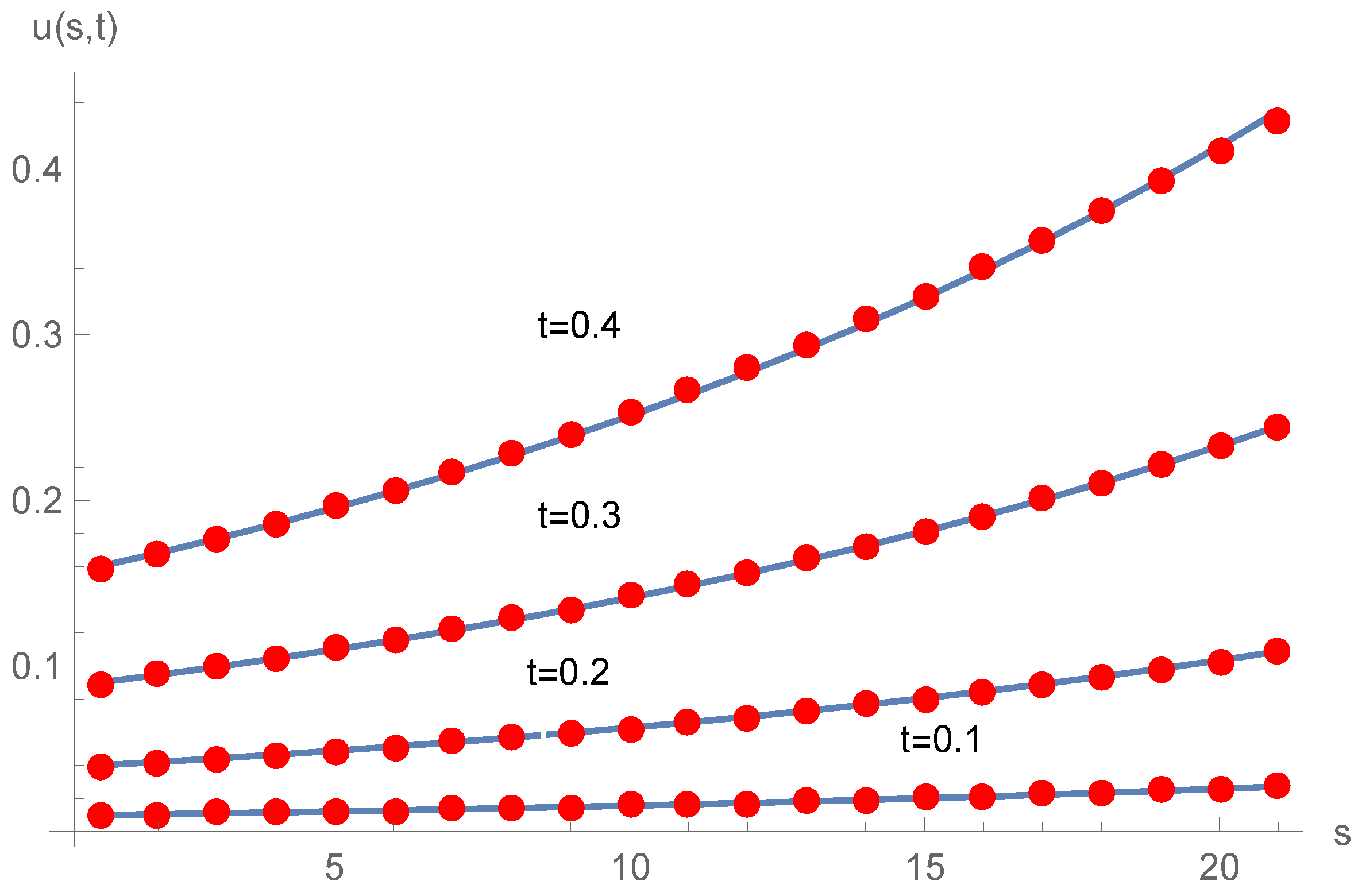Figure 1 illustrates the graph of numerical and exact values for time levels $t=0.4$, $0.3$, $t=0.2$ and $t=0.1$. 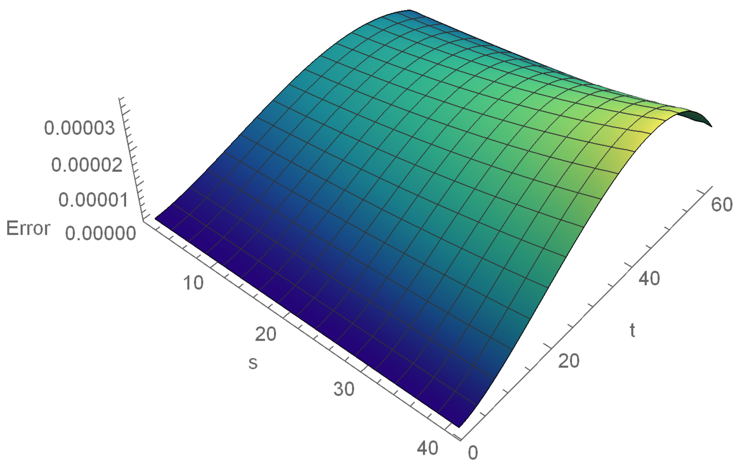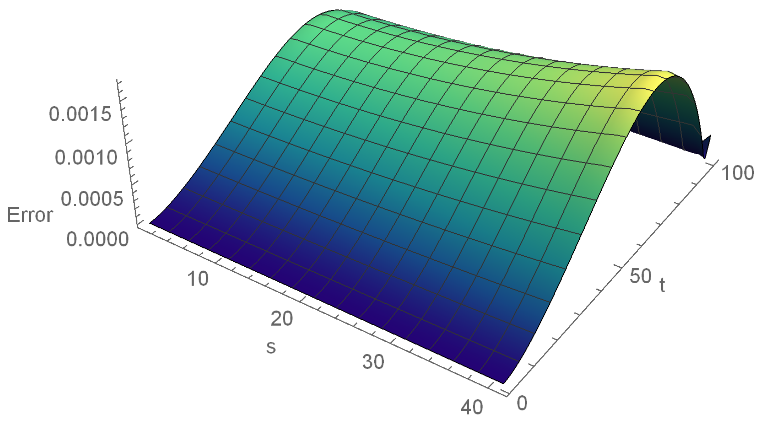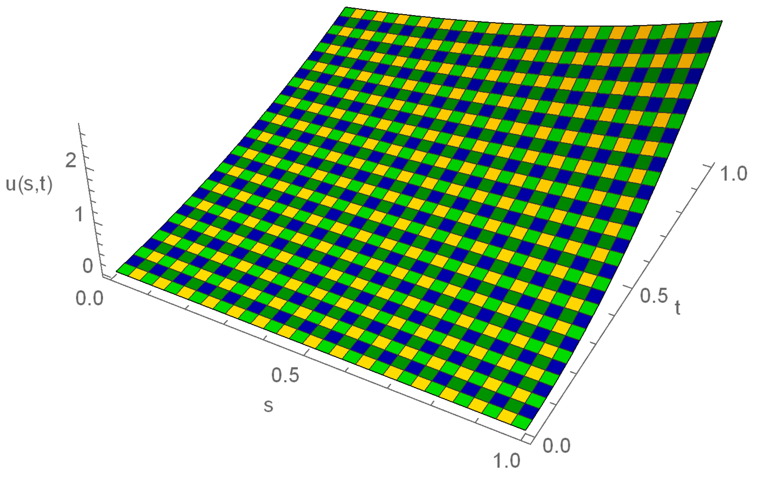Error graph for $\alpha =0.8$, $N=40$, at $t=0.1$ is plotted in Figure 2. Numerical solutions given by MECBS is plotted in Figure 3 corresponding $\alpha =0.7$ and $T=1$.

Table 1. Error norms of example 1 for $\alpha =0.9$, $\tau =0.003$ at $t=0.18$.

M	Method in [2]		MECBS
	${\mathit{E}}_{\mathit{\infty }}$	RMSE	${\mathit{E}}_{\mathit{\infty }}$	RMSE	CPU Time
06	0.0004175	0.0001734	0.0003592	0.0000388	0.023125
11	0.0003690	0.0001118	0.0003329	0.0000200	0.093750
21	0.0001256	0.0000298	0.0000973	0.0000032	0.156250
41	0.0000174	0.0000064	0.0000646	0.0000011	0.390625

Table 2. Comparison of RMSE for $\alpha =0.8$, $M=21$ at $t=0.18$.

$\mathit{\tau }$	Method in [2]
	Gaussian	Inverse Quadratic	Inverse Multi Quadratic	MECBS	CPU Time
$\frac{1}{50}$	0.000018177	0.000018192	0.000018126	0.000013528	0.45313
$\frac{1}{100}$	0.000008112	0.000008128	0.000008066	0.000007219	1.43750
$\frac{1}{200}$	0.000003621	0.000003637	0.000003578	0.000003547	1.48438
$\frac{1}{400}$	0.000001645	0.000001660	0.000001611	0.000001652	9.93750

Table 3. The errors for $\alpha =0.7$, $M=50$, $t=0.3$ at different $\tau$.

$\mathit{\tau }$	${\mathit{E}}_{\mathit{\infty }}$	${\mathit{E}}_2$	RMSE	O
$\frac{1}{5}$	0.01124290	0.001260777	0.0001765441	…
$\frac{1}{10}$	0.00420084	0.000466420	0.0000653119	1.42027
$\frac{1}{20}$	0.00157882	0.000167477	0.0000234515	1.41183
$\frac{1}{40}$	0.00059535	0.000051284	0.0000071812	1.40705

Table 4. The $E_{\infty }$, $E_2$ and RMSE of Example 1 for $\alpha =0.75$, $\tau =50$ at $t=0.1$.

M	${\mathit{E}}_{\mathit{\infty }}$	${\mathit{E}}_2$	RMSE	O
$\frac{1}{5}$	0.000112879	0.0000343788	0.0000140351	…
$\frac{1}{10}$	0.000026850	0.0000048482	0.0000014618	2.071799
$\frac{1}{20}$	0.000006615	0.0000008568	0.0000001870	2.021091
$\frac{1}{40}$	0.000001504	0.0000001627	0.0000000254	2.136861

Figure 1. Comparison graph of Example 1 at $\alpha =0.8$.

Figure 2. Error plot corresponding $\alpha =0.8$, $N=40$ at $t=0.1$ for Example 1.

Figure 3. Space-time graph corresponding $\alpha =0.7$, $\gamma =10$, ${\gamma }_1=1$ and ${\gamma }_3=1$.

Example 2.

The following form of FTE

$$\frac{{\partial }^{2\alpha }u(s,t)}{\partial t^{2\alpha }}+20\frac{{\partial }^{\alpha }u(s,t)}{\partial t^{\alpha }}-\frac{{\partial }^{2}u(s,t)}{\partial s^2}+u^3(s,t)+u(s,t)=g(s,t),$$

with

$$\left\{\begin{array}{c}u(s,0)=0,0\le s\le 1\hfill \\ u_t(s,0)=0,\hfill \\ u(0,t)=2t^{2+\alpha },t\ge 0\hfill \\ u(1,t)=2t^{2+\alpha }cosh\left(1\right).\hfill \end{array}\right.$$

where $g(s,t)=\frac{2\mathsf{\Gamma }(3+\alpha )}{\mathsf{\Gamma }(3-\alpha )}{t}^{2-\alpha }cosh\left(x\right)+20\mathsf{\Gamma }(3+\alpha )t^{2}cosh\left(x\right)-2t^{2+\alpha }cosh\left(x\right)+{\gamma }_1{(2t^{2+\alpha }cosh\left(x\right))}^3+2{\gamma }_{3}2t^{2+\alpha }cosh\left(x\right)$ and analytical solution is $u(s,t)=2t^{2+\alpha }cosh\left(x\right)$ [2].

Table 5 presents the comparison of $E_2$ and RMSE with CPU time for $\alpha =0.7$, $M=17$ and various values of $\tau$ at $t=0.4$. In Table 6, $E_{\infty }$, $E_2$, RMSE and rate of convergence are given for several values of $\tau$, $\alpha =0.8$, $M=20$ at $t=0.4$. Table 7 and Table 8 demonstrate that the numerical outcomes and exact values for $\alpha =0.6$, $0.7$, $0.8$ and $0.9$ at several knots. 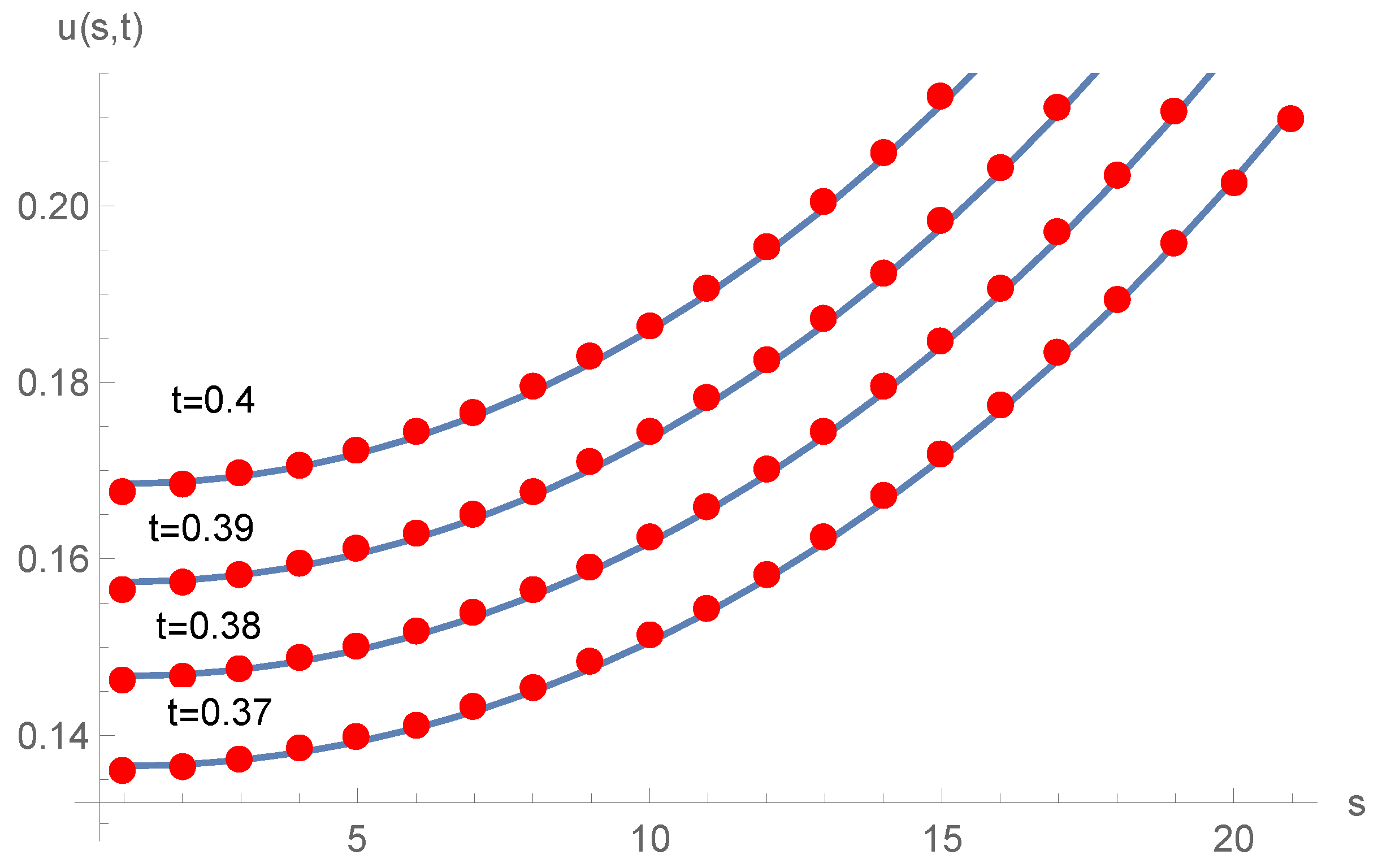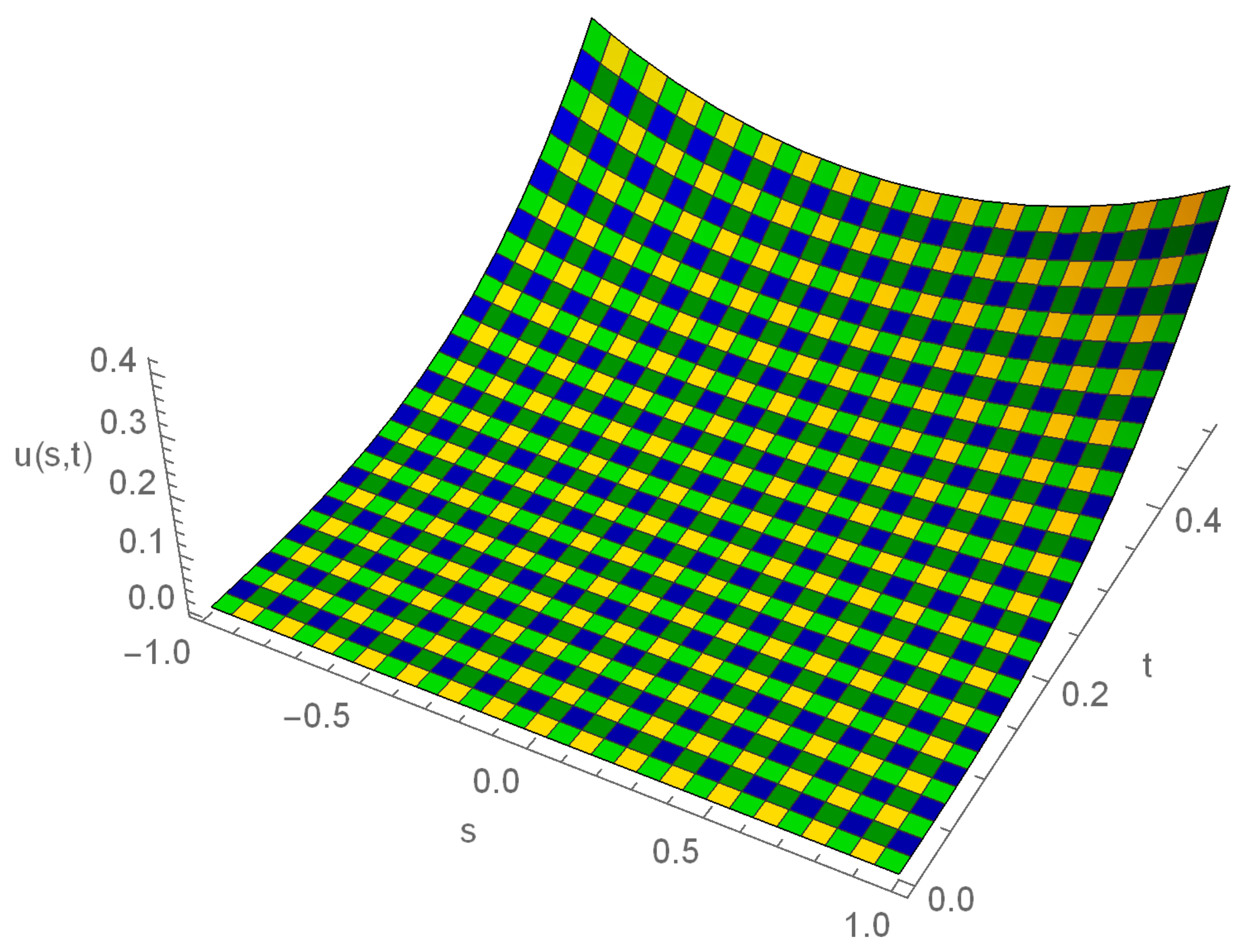Figure 4 shows the computational outcomes and exact solutions for various time steps. Figure 5 and Figure 6 depict the error plot and space-time graph of Example 2 at $t=0.6$ and $0.5$ respectively.

Table 5. The $E_2$ and RMSE of Example 2 for $\alpha =0.7$, $M=17$ at $t=0.4$.

$\mathit{\tau }$	Method in [2]				MECBS
	${\mathit{E}}_2$	RMSE	${\mathit{E}}_2$	RMSE	${\mathit{E}}_2$	RMSE	CPU Time
0.008	0.0019484	0.0004726	0.0019501	0.0004730	0.00038535	0.000090827	0.28125
0.004	0.0009842	0.0002387	0.0009860	0.0002391	0.00017451	0.000041133	1.29688
0.002	0.0004949	0.0001200	0.0004968	0.0001205	0.00014626	0.000034473	5.50000
0.001	0.0002481	0.0000602	0.0002502	0.0000607	0.00013846	0.000032635	23.9375

Table 6. The errors of Example 2 for $\alpha =0.8$, $M=20$, $t=0.4$ at different $\tau$.

$\mathit{\tau }$	${\mathit{E}}_{\mathit{\infty }}$	${\mathit{E}}_2$	RMSE	O
$\frac{1}{5}$	0.0432554	0.00796291	0.00173765	…
$\frac{1}{10}$	0.0192807	0.00363394	0.00079299	1.16572
$\frac{1}{20}$	0.0085208	0.00164049	0.00035799	1.17809
$\frac{1}{40}$	0.0037512	0.00072265	0.00015770	1.18365
$\frac{1}{80}$	0.0016524	0.00030803	0.00006722	1.18277

Table 7. Numerical and exact values for $\alpha =0.6$, $0.7$ at knots.

s	$\mathit{\alpha }=0.6$		$\mathit{\alpha }=0.7$
	Numerical Values	Exact Values	Numerical Values	Exact Values
0.0	0.0871566	0.0874068	0.0777292	0.0774921
0.1	0.0879147	0.0878442	0.0783412	0.0778799
0.2	0.0893033	0.0891608	0.0795512	0.0790471
0.3	0.0915300	0.0913697	0.0815268	0.0810055
0.4	0.0946615	0.0944931	0.0843142	0.0837746
0.5	0.0987382	0.0985622	0.0879450	0.0873821
0.6	0.1038020	0.1036180	0.0924559	0.0918642
0.7	0.1099020	0.1097100	0.0978915	0.0972657
0.8	0.1170840	0.1169010	0.1043004	0.1036410
0.9	0.1253520	0.1252620	0.1117061	0.1110530
1.0	0.1344900	0.1348760	0.1199427	0.1195770

Table 8. Numerical values and exact values for $\alpha =0.8$, $0.9$ at knots.

s	$\mathit{\alpha }=0.8$		$\mathit{\alpha }=0.9$
	Numerical Values	Exact Values	Numerical Values	Exact Values
0.0	0.0694043	0.0687020	0.0621345	0.0609090
0.1	0.0697533	0.0690458	0.0624465	0.0612138
0.2	0.0707987	0.0700806	0.0633824	0.0621313
0.3	0.0725527	0.0718169	0.0649526	0.0636705
0.4	0.0750328	0.0742719	0.0671730	0.0658471
0.5	0.0782639	0.0774702	0.0700656	0.0686826
0.6	0.0822783	0.0814439	0.0736595	0.0722055
0.7	0.0871162	0.0862326	0.0779906	0.0764511
0.8	0.0928260	0.0918845	0.0831022	0.0814619
0.9	0.0994647	0.0984559	0.0890456	0.0872879
1.0	0.1070960	0.1060130	0.0958785	0.0939875

Figure 4. Comparison graph of Example 2 at $\alpha =0.7$.

Figure 5. Error plot of Example 2 for $\alpha =0.85$, $N=40$ at $t=0.6$.

Figure 6. Space-time plot for $\alpha =0.8$, $\gamma =20$, ${\gamma }_1=1$, ${\gamma }_3=1$ at $t=0.5$.

7. Conclusions

In this article, a MECBS collocation technique was presented for the numerical solution of nonlinear FTE. The Crank–Nicolson and MECBS were employed for the discretization of space dimension. Time variable is discretized by finite difference scheme in Caputo’s sense. This method has $2-\alpha$ order accurate in time direction and order 2 accurate in space dimension consequently MECBS lead to accurate numerical outcomes. The MECBS collocation technique has been validated through several illustrative numerical experiments.