Solution and Interpretation of Neutrosophic Homogeneous Difference Equation

Abstract

In this manuscript, we focus on the brief study of finding the solution to and analyzingthe homogeneous linear difference equation in a neutrosophic environment, i.e., we interpreted the solution of the homogeneous difference equation with initial information, coefficient and both as a neutrosophic number. The idea for solving and analyzing the above using the characterization theorem is demonstrated. The whole theoretical work is followed by numerical examples and an application in actuarial science, which shows the great impact of neutrosophic set theory in mathematical modeling in a discrete system for better understanding the behavior of the system in an elegant manner. It is worthy to mention that symmetry measure of the systems is employed here, which shows important results in neutrosophic arena application in a discrete system.

1. Introduction

1.1. Uncertainty Theory and Neutrosophic Sets

The uncertainty theory becomes a very helpful tool for real life modeling in discrete and continuous systems. The different theories of the fuzzy uncertainty theory have been given a new direction since the setting of the fuzzy set, invented by Professor Zadeh [1]. This is generalized representation of [1] is established as an intuitionistic fuzzy set theory by Atanassov [2]. Atarasov gave a novel designusing the intuitionistic fuzzy theory, where he demonstrated the idea of a membership function and non-membership function by which degree of belongingness and non-belongingness, respectively, can be measured in a set. Liu and Yuan [3] ignited the perception of a triangular intuionistic fuzzy set, which is the affable blend of a triangular fuzzy number and a intuionistic fuzzy set theory. Ye [4] set up the idea for a trapezoidal intuionistic fuzzy set. Smarandache [5] found his more generalized idea as a neutrosophic set, considering terms of the truth membership function, the indeterminacy membership function, and the falsity membership function. This theory become more beneficial and germane, rather than the common fuzzy and intuitionistic fuzzy theory settings.

Several researchershave already worked in the neutrosophic field, some of which have developed the theory [6,7], while some have applied the related theories in an applied field [8,9]. Various kinds of forms and extensions of the Neutrosophic set, such as the triangular neutrosophic set [10], the bipolar neutrosophic sets [11,12,13,14], and the multi-valued neutrosophic sets [15], were also found.

1.2. Difference Equation in an Uncertain Environment

There exist some works associated with difference equation and uncertainty. Mostly, researchers have worked on the difference equation allied with fuzzy and intuitionistic fuzzy environments. We are now giving details descriptions of some related published work. In the literature [16], Deebaet al. found a strategy for solving the fuzzy difference equation with an interesting application. The model involving CO2 levels in blood streamflow is thinkingin the view ofthe fuzzy difference equation by Deebaet al. [17]. Lakshmikantham and Vatsala [18] talk abou tdifferent basic theories and properties of fuzzy difference equations. Papaschinopoulos et al. [19,20] and PapaschinopoulosandSchinas [21] discuss more findings in a similar context. Papaschinopoulos and Stefanidou [22] provide an explanation on boundedness with asymptotic behavior of a fuzzy difference equation. Umekkanet al. [23] give a finance application based on discrete system modeling in a fuzzy environment. Stefanidou et al. [24] treat the exponential-type fuzzy difference equation. The asymptotic behavior of a second order fuzzy difference equation is considered by Din [25]. The fuzzy non-linear difference equation is considered by Zhang et al. [26], where Memarbashi and Ghasemabadi [27] corporate with a volterra type rational form by Stefanidou and Papaschinopoulos [28]. The economics application is considered by Konstantinos et al. [29]. Mondal et al. [30] solve the second-order intuitionistic difference equation. Non-linear interval-valued fuzzy numbers and their relevance to difference equations are shown in [31]. National income determination models with fuzzy stability analysis in a discrete system are elaborately discussed by Sarkar et al. [32]. The fuzzy discrete logistic equation is taken and stability situations are found in the literature [33]. Zhang et al. [34] show the asymptotic performance of a discrete time fuzzy single species population model. On discrete time, a Beverton–Holt population replica with fuzzy environment is illustrated in [35]. Additionally, a different view of the fuzzy discrete logistic equation is taken under uncertainty in [36]. The existence and stability situation of the difference equation with a fuzzy setting is found by Mondal et al. [37]. Important results are also found for fuzzy difference equations by Khastan and Alijani [38] and Khastan [39].

1.3. Novelties of the Work

In this connection of the above idea, few advances can still be prepared, which include:

(1)

The homogeneous difference equation, solved and analyzed with a neutrosophic initial condition, neutrosophic coefficient, and neutrosophic coefficient and initial together as a different section, which was not done earlier.

(2)

Establishment of the corresponding characterization theorem for the neutrosophic set with a difference equation.

(3)

Different theorems, lemmas, and corollary drawn for the purpose of the study.

(4)

Numerical examples of the difference equation with a neutrosophic number, solved and illustrated for better understanding of our observations.

(5)

An application in actuarial science, illustrated in a neutrosophic environment for better understanding of the practical application of the proposed theoretical results.

1.4. Structure of the Paper

In Section 1, we recall the related work and write the novelties of our study. The preliminary concepts are addressed in Section 2. The difference equation with a neutrosophic variable is defined and corresponds with a necessary theory, for which a lemma is prepared for the study in Section 3. Section 4 shows the solution of the neutrosophic homogeneous difference equation. Two numerical examples are shown in Section 5. In Section 6, we take an appliance of an actuarial science problem in the neutrosophic data and solve it. The conclusion and future research scope are written in Section 7.

2. PreliminaryIdea

Definition 1.

Neutrosophicset: [6] Let X be a universe set. A single-valued neutrosophic set A on X is distinct as $A=\left\{\left(T_A\left(x\right),I_A\left(x\right),F_A\left(x\right)\right):x\in X\right\}$, where $T_A\left(x\right),I_A\left(x\right),F_A\left(x\right):X\to \left[0,1\right]$ is the degree of membership, degree of indeterministic, and degree of non-membership, respectively, of the element $x\in X$, such that $0\le T_A\left(x\right)+I_A\left(x\right)+F_A\left(x\right)\le 3$.

Definition 2.

Neutrosophicfunction: If we take the set of all real numbers as notation $\mathcal{R}$ and real valued fuzzy numbers as notation ${\mathcal{R}}_{\mathcal{F}}$, then the function $W:\mathcal{R}\to \left[0,1\right]$ is called a fuzzy number valued function if $w$ satisfies the subsequent properties.

(1)

$W$ is the upper semi continuous.

(2)

$W$ is the fuzzy convex, i.e., $W\left(\lambda s_1+\left(1-\lambda \right)s_2\right)\ge min\left\{W\left(s_1\right),W\left(s_2\right)\right\}$ for all $s_1,s_2\in \mathcal{R}$ and $\lambda \in \left[0,1\right]$.

(3)

$W$ is normal, i.e., $\exists$ a $s_0\in \mathcal{R},$ such that $W\left(s_0\right)=1$

(4)

Closure of $supp\left(W\right)$ is compact, where $supp\left(W\right)=\left\{s\in \mathcal{R}|W\left(s\right)>0\right\}$.

Definition 3.

Triangular neutrosophic number: [40] If we consider the measure of the truth, for which indeterminacy and falsity are not dependent, then a Triangular Neutrosophic number is taken as $\tilde{\mathit{N}}=\left({\mathit{r}}_{\mathbf{0}},{\mathit{r}}_{\mathbf{1}},{\mathit{r}}_{\mathbf{2}};{\mathit{s}}_{\mathbf{0}},{\mathit{s}}_{\mathbf{1}},{\mathit{s}}_{\mathbf{2}};{\mathit{w}}_{\mathbf{0}},{\mathit{w}}_{\mathbf{1}},{\mathit{w}}_{\mathbf{2}}\right),$ where the truth membership, falsity, and indeterminacy membership function is treated as follows:

$$T_{\tilde{\mathrm{N}}}\left(y\right)=\{\begin{array}{c}\begin{array}{cc}\frac{y-r_0}{r_1-r_0}& \mathrm{when}{r}_0\le y<r_1\end{array}\\ \begin{array}{cc}1& \mathrm{when}y=r_1\end{array}\\ \begin{array}{c}\begin{array}{cc}\frac{r_2-y}{r_2-r_1}& \mathrm{when}{r}_1<y\le r_2\end{array}\\ \begin{array}{cc}0& \mathrm{otherwise}\end{array}\end{array}\end{array}$$

and

$$F_{\tilde{\mathrm{N}}}\left(y\right)=\{\begin{array}{c}\begin{array}{cc}\frac{s_1-y}{s_1-s_0}& \mathrm{when}{s}_0\le y<s_1\end{array}\\ \begin{array}{cc}0& \mathrm{when}y=s_1\end{array}\\ \begin{array}{c}\begin{array}{cc}\frac{y-s_1}{s_2-s_2}& \mathrm{when}{s}_1<y\le s_2\end{array}\\ \begin{array}{cc}1& \mathrm{otherwise}\end{array}\end{array}\end{array}$$

$$I_{\tilde{\mathrm{N}}}\left(y\right)=\{\begin{array}{c}\begin{array}{cc}\frac{w_1-y}{w_1-w_0}& \mathrm{when}{w}_0\le y<w_1\end{array}\\ \begin{array}{cc}0& \mathrm{when}y=w_1\end{array}\\ \begin{array}{c}\begin{array}{cc}\frac{y-w_1}{w_2-w_1}& \mathrm{when}{w}_1<y\le w_2\end{array}\\ \begin{array}{cc}1& \mathrm{otherwise}\end{array}\end{array}\end{array}$$

where$0\le T_{\tilde{\mathrm{N}}}\left(y\right)+F_{\tilde{\mathrm{N}}}\left(y\right)+I_{\tilde{\mathrm{N}}}\left(y\right)\le 1$, $y\in \tilde{\mathrm{N}}$.

The parametric setting of the above number is ${\left(\tilde{\mathrm{N}}\right)}_{\alpha ,\beta ,\gamma }=\left[T_{Neu1}\left(\alpha \right),T_{Neu2}\left(\alpha \right);I_{Neu1}\left(\beta \right),I_{Neu2}\left(\beta \right);F_{Neu1}\left(\gamma \right),F_{Neu2}\left(\gamma \right)\right]$,

where

$$N_L^1\left(\alpha \right)=r_0+\alpha \left(r_1-r_0\right)$$

$$N_R^1\left(\alpha \right)=r_2-\alpha \left(r_2-r_1\right)$$

$$N_L^2\left(\beta \right)=s_1-\beta \left(s_1-s_0\right)$$

$$N_R^2\left(\beta \right)=s_1+\beta \left(s_2-s_1\right)$$

$$N_L^3\left(\gamma \right)=w_1-\gamma \left(w_1-w_0\right)$$

$$N_R^3\left(\gamma \right)=w_1+\gamma \left(w_2-w_1\right)$$

Here, $0<\alpha ,\beta ,\gamma \le 1$ and $0<\alpha +\beta +\gamma \le 3$

The verbal phrase with the number can be written as in

Table 1. The verbal phrase of different uncertain settings and neutrosophic numbers.

Type of Uncertain Parameter	Verbal Phrase	Used Functionsand Their Roles
Triangular Fuzzy Number	[Low, Medium, High]	Membership function for measuring degree of belongingness
Triangular Intuitionistic Fuzzy Number	[Low, Medium, High; Very Low, Medium, Very High]	Membership and non-membership function for measuring degree of belongingness and non-belongingness
Triangular NeutrosophicNumber	[Low, Medium, High; Very Low, Medium, Very High; Between low and very low; Medium; Between high and very high]	Truthiness, falsity, and indeterminacy function for measuring the degree of truth belongingness, strictly non-belongingness and indeterminacy

:

Definition 4.

Hukuhara difference on neutrosophic function: Let $E^{*}$ be the set of all neutrosophicfunctions, $\tilde{s},\tilde{t}\in E^{*}$. If $\exists$ is a neutrosophic number, $\tilde{w}\in E^{*}$ and $\tilde{w}$ suit the relation $\tilde{s}=\tilde{w}+\tilde{t}$, then $\tilde{w}$ is assumed to be the Hukuhara difference of $\tilde{s}$ and $\tilde{t}$, denoted by $\tilde{w}=\tilde{s}\ominus \tilde{t}$.

3. Difference Equation with a Neutrosophic Variable

Definition 5.

A difference equation (sometime named as a recurrence relation) is an equation that relates the consecutive terms of a sequence of numbers.

A $q$th order difference equation in the linear form can be articulated:

$$x_{n+q}=d_1{x}_{n+q-1}+d_2{x}_{n+q-2}+\cdots +d_q{x}_n+b_n$$

(1)

where $d_1,d_2,\dots ,d_q$ and $b_n$ are constants, which are known.

If $b_n=0$ for all $n$, then Equation (1) is the homogeneous difference equation. On the other hand, it will be the non-homogeneous difference equation if $b_n\ne 0$, where $b_n$ is treated as the forcing factor.

We consider an autonomous linear homogeneous difference equation of the form:

$$x_{n+1}=\sigma x_n,\left(\sigma \ne 0\right)$$

(2)

with the initial condition $x_{n=0}=x_0$. The solution of Equation (2) can then be written as:

$$x_n={\sigma }^n{x}_0$$

(3)

Theorem 1.

[41]Let $m\in \mathbb{N},m\ge 2$. A linear homogeneous system of them first order difference equation is given in matrix form as:

$$X_{n+1}=A{X}_n$$

(4)

where,$X_n={\left(X_n^1,X_n^2,\dots ,X_n^m\right)}^T$and$A={\left(a_{ij}\right)}_{m\times m},i,j=1,2,\dots ,m$

The solution of Equation (3) can then be written as:

$$X_n=A^n{X}_0,n\in \mathbb{N}$$

(5)

The difference Equation (1) is considered as the neutrosophic difference equation if any one of the following conditions are added:

(i)

The initial condition or conditions are the neutrosophic number (Type I);

(ii)

The coefficient or coefficients are the neutrosophic number (Type II);

(iii)

The initial conditions and coefficient or the coefficients are both neutrosophic numbers (Type III).

Theorem 2.

Characterization theorem: Let us consider the neutrosophic difference equation problem:

$${\tilde{x}}_{n+1}=\tilde{f}\left(x_n,n\right),$$

(6)

with initial value${\tilde{x}}_{n=0}={\tilde{x}}_0$as a neutrospohic number, where$f:E^{*}\times {\mathbb{Z}}_{\ge 0}\to E^{*}$, such that

(1) 

The parametric form of the function is:

$${\left[\tilde{f}\left(\left(x_n,n\right)\right)\right]}_{\left(\alpha ,\beta ,\gamma \right)}=\left[\begin{array}{c}{f}_{L,n}^1\left(x_{L,n}^1\left(\alpha \right),x_{R,n}^1\left(\alpha \right),n,\alpha \right),f_{R,n}^1\left(x_{L,n}^1\left(\alpha \right),x_{R,n}^1\left(\alpha \right),n,\alpha \right);\\ f_{L,n}^2\left(x_{L,n}^2\left(\beta \right),x_{R,n}^2\left(\beta \right),n,\beta \right),f_{R,n}^2\left(x_{L,n}^2\left(\beta \right),x_{R,n}^2\left(\beta \right),n,\beta \right);\\ f_{L,n}^3\left(x_{L,n}^3\left(\gamma \right),x_{R,n}^3\left(\gamma \right),n,\gamma \right),f_{R,n}^3\left(x_{L,n}^3\left(\gamma \right),x_{R,n}^3\left(\gamma \right),n,\gamma \right)\end{array}\right]$$

(2) 

The functions$f_{L,n}^1\left(x_{L,n}^1\left(\alpha \right),x_{R,n}^1\left(\alpha \right),n,\alpha \right)$,$f_{R,n}^1\left(x_{L,n}^1\left(\alpha \right),x_{R,n}^1\left(\alpha \right),n,\alpha \right)$,$f_{L,n}^2\left(x_{L,n}^2\left(\beta \right),x_{R,n}^2\left(\beta \right),n,\beta \right)$,$f_{R,n}^2\left(x_{L,n}^2\left(\beta \right),x_{R,n}^2\left(\beta \right),n,\beta \right)$,$f_{L,n}^3\left(x_{L,n}^3\left(\gamma \right),x_{R,n}^3\left(\gamma \right),n,\gamma \right)$and$f_{R,n}^3\left(x_{L,n}^3\left(\gamma \right),x_{R,n}^3\left(\gamma \right),n,\gamma \right)$are taken as continuous functions, i.e., for any${\in }_1>0\exists$a${\delta }_1>0$, such that:

$$\left|f_{L,n}^1\left(x_{L,n}^1\left(\alpha \right),x_{R,n}^1\left(\alpha \right),n,\alpha \right)-f_{L,n_1}^1\left(x_{L,n_1}^1\left(\alpha \right),x_{R,n_1}^1\left(\alpha \right),n_1,\alpha \right)\right|<{\in }_1$$

for all$\alpha \in \left[0,1\right]$

with$\Vert \left(x_{L,n}^1\left(\alpha \right),x_{R,n}^1\left(\alpha \right),n,\alpha \right)-\left(x_{L,n_1}^1\left(\alpha \right),x_{R,n_1}^1\left(\alpha \right),n_1,\alpha \right)\Vert <{\delta }_1$and for any${\in }_2>0\exists$an${\delta }_2>0$, such that:

$$\left|f_{R,n}^1\left(x_{L,n}^1\left(\alpha \right),x_{R,n}^1\left(\alpha \right),n,\alpha \right)-f_{R,n_2}^1\left(x_{L,n_2}^1\left(\alpha \right),x_{R,n_2}^1\left(\alpha \right),n_2,\alpha \right)\right|<{\in }_2\mathrm{for}\mathrm{all}\alpha \in \left[0,1\right]$$

with$\Vert \left(x_{L,n}^1\left(\alpha \right),x_{R,n}^1\left(\alpha \right),n,\alpha \right)-\left(x_{L,n_2}^1\left(\alpha \right),x_{R,n_2}^1\left(\alpha \right),n_2,\alpha \right)\Vert <{\delta }_2$, where$n,n_1$and$n_2\in {\mathbb{Z}}_{\ge 0}$.

In a similar way, the continuity of the remaining four functions, $f_{L,n}^2\left(x_{L,n}^2\left(\beta \right),x_{R,n}^2\left(\beta \right),n,\beta \right)$, $f_{R,n}^2\left(x_{L,n}^2\left(\beta \right),x_{R,n}^2\left(\beta \right),n,\beta \right)$, $f_{L,n}^3\left(x_{L,n}^3\left(\gamma \right),x_{R,n}^3\left(\gamma \right),n,\gamma \right)$ and $f_{R,n}^3\left(x_{L,n}^3\left(\gamma \right),x_{R,n}^3\left(\gamma \right),n,\gamma \right)$, can be defined.

The difference Equation (6) then reduces to the system of six difference equations, as follows:

$$x_{L,n+1}^1\left(\alpha \right)=f_{L,n}^1\left(x_{L,n}^1\left(\alpha \right),x_{R,n}^1\left(\alpha \right),n,\alpha \right)$$

$$x_{R,n+1}^1\left(\alpha \right)=f_{R,n}^1\left(x_{L,n}^1\left(\alpha \right),x_{R,n}^1\left(\alpha \right),n,\alpha \right)$$

$$x_{L,n+1}^2\left(\beta \right)=f_{L,n}^2\left(x_{L,n}^2\left(\beta \right),x_{R,n}^2\left(\beta \right),n,\beta \right)$$

$$x_{R,n+1}^2\left(\beta \right)=f_{R,n}^2\left(x_{L,n}^2\left(\beta \right),x_{R,n}^2\left(\beta \right),n,\beta \right)$$

$$x_{L,n+1}^3\left(\gamma \right)=f_{L,n}^3\left(x_{L,n}^3\left(\gamma \right),x_{R,n}^3\left(\gamma \right),n,\gamma \right)$$

$$x_{R,n+1}^3\left(\gamma \right)=f_{R,n}^3\left(x_{L,n}^3\left(\gamma \right),x_{R,n}^3\left(\gamma \right),n,\gamma \right)$$

with the initial conditions:

$$x_{L,n=0}^1\left(\alpha \right)=x_{L,0}^1\left(\alpha \right)$$

$$x_{R,n=0}^1\left(\alpha \right)=x_{R,0}^1\left(\alpha \right)$$

$$x_{L,n=0}^1\left(\beta \right)=x_{L,0}^1\left(\beta \right)$$

$$x_{R,n=0}^1\left(\beta \right)=x_{R,0}^1\left(\beta \right)$$

$$x_{L,n=0}^1\left(\gamma \right)=x_{L,0}^1\left(\gamma \right)$$

$$x_{R,n=0}^1\left(\gamma \right)=x_{R,0}^1\left(\gamma \right)$$

Note 1.

By the characterization theorem, we can see that a neutrosopic difference equation is transformed into a system of six difference equations in crisp form. In this article, we have taken only a single neutrosophic difference equation in a neutrosophic environment. Hence, the difference equation converted into six crisp difference equations.

Definition 6.

Strong and weak solutions of a neutrosophic difference equation: The solutions of difference Equation (6), with initial condition (3.7) to be regarded as:

(1) 

A strong solution if

$$x_{L,n}^1\left(\alpha \right)\le x_{R,n}^1\left(\alpha \right)$$

$$x_{L,n}^1\left(\beta \right)\le x_{R,n}^1\left(\beta \right)$$

$$x_{L,n}^1\left(\gamma \right)\le x_{R,n}^1\left(\gamma \right)$$

and

$$\frac{\partial }{\partial \alpha }\left[x_{L,n}^1\left(\alpha \right)\right]>0,\frac{\partial }{\partial \alpha }\left[x_{R,n}^1\left(\alpha \right)\right]<0$$

$$\frac{\partial }{\partial \beta }\left[x_{L,n}^1\left(\beta \right)\right]<0,\frac{\partial }{\partial \beta }\left[x_{R,n}^1\left(\beta \right)\right]>0$$

$$\frac{\partial }{\partial \gamma }\left[x_{L,n}^1\left(\gamma \right)\right]<0,\frac{\partial }{\partial \gamma }\left[x_{R,n}^1\left(\gamma \right)\right]>0$$

for every$\alpha ,\beta ,\gamma \in \left[0,1\right]$.

(2) 

A weak solution if

$$x_{L,n}^1\left(\alpha \right)\ge x_{R,n}^1\left(\alpha \right)$$

$$x_{L,n}^1\left(\beta \right)\ge x_{R,n}^1\left(\beta \right)$$

$$x_{L,n}^1\left(\gamma \right)\ge x_{R,n}^1\left(\gamma \right)$$

and

$$\frac{\partial }{\partial \alpha }\left[x_{L,n}^1\left(\alpha \right)\right]<0,\frac{\partial }{\partial \alpha }\left[x_{R,n}^1\left(\alpha \right)\right]>0$$

$$\frac{\partial }{\partial \beta }\left[x_{L,n}^1\left(\beta \right)\right]>0,\frac{\partial }{\partial \beta }\left[x_{R,n}^1\left(\beta \right)\right]<0$$

$$\frac{\partial }{\partial \gamma }\left[x_{L,n}^1\left(\gamma \right)\right]>0,\frac{\partial }{\partial \gamma }\left[x_{R,n}^1\left(\gamma \right)\right]<0$$

for every$\alpha ,\beta ,\gamma \in \left[0,1\right]$.

Definition 7.

Let $pandq$ be neutrosophic numbers, where ${\left[\tilde{p}\right]}_{\left(\alpha ,\beta ,\gamma \right)}=\left[p_L^1\left(\alpha \right),p_R^1\left(\alpha \right);p_L^2\left(\beta \right),p_R^2\left(\beta \right);p_L^3\left(\gamma \right),p_R^3\left(\gamma \right)\right]$, ${\left[\tilde{q}\right]}_{\left(\alpha ,\beta ,\gamma \right)}=\left[q_L^1\left(\alpha \right),q_R^1\left(\alpha \right);q_L^2\left(\beta \right),q_R^2\left(\beta \right);q_L^3\left(\gamma \right),q_R^3\left(\gamma \right)\right]$, for all $\alpha ,\beta ,\gamma \in [0,1]$. The metric on the neutrosophic number space is then defined as:

$$d\left(p,q\right)=sup\underset{\alpha ,\beta ,\gamma \in \left[0,1\right]}{\max }\left\{\left|p_L^1\left(\alpha \right)-q_L^1\left(\alpha \right)\right|,\left|p_R^1\left(\alpha \right)-q_R^1\left(\alpha \right)\right|,\left|p_L^2\left(\beta \right)-q_L^2\left(\beta \right)\right|,\left|p_R^2\left(\beta \right)-q_R^2\left(\beta \right)\right|,\left|p_L^3\left(\gamma \right)-q_L^3\left(\gamma \right)\right|,\left|p_R^3\left(\gamma \right)-q_R^3\left(\gamma \right)\right|\right\}.$$

Note 2.

For some cases, the solution may not become strictly strong or weak solution type. In this scenario, a specific time interval or specific interval of$\mathsf{\alpha },\mathsf{\beta }$, or$\mathsf{\gamma }$becomes the strong or weak solution. The main objective is to find the strong solutions. For scenariosin which neitherthe strong nor weak solutions occur, we call them non-recommended neutrosophic solutions. We strongly recommended taking strong solutions.

4. Solution of Neutrosophic Homogeneous Difference Equation

Considering linear homogeneous difference equations:

$$u_{n+1}=a{u}_n$$

(7)

In a neutrosophic sense, another inequivalent form of is (7) taken as:

$$u_{n+1}-a{u}_n=0$$

(8)

Remarks 1.

Equations (7) and (8) are equivalent in a crisp sense, but in fuzzy sense they are not equivalent.

Proof 1. 

If we take the fuzzy difference Equation (7), it becomes Theorem 1.

$${\left[u_{n+1}\right]}_{\left(\alpha ,\beta ,\gamma \right)}={\left[a{u}_n\right]}_{\left(\alpha ,\beta ,\gamma \right)}$$

or

$$\left[u_{L,n+1}^1\left(\alpha \right),u_{R,n+1}^1\left(\alpha \right);u_{L,n+1}^2\left(\beta \right),u_{R,n+1}^2\left(\beta \right);u_{L,n+1}^3\left(\gamma \right),u_{R,n+1}^3\left(\gamma \right)\right]=a\left[\left[u_{L,n}^1\left(\alpha \right),u_{R,n}^1\left(\alpha \right);u_{L,n}^2\left(\beta \right),u_{R,n}^2\left(\beta \right);u_{L,n}^3\left(\gamma \right),u_{R,n}^3\left(\gamma \right)\right]\right],$$

i.e.,

$$\{\begin{array}{c}{u}_{L,n+1}^1\left(\alpha \right)=a{u}_{L,n}^1\left(\alpha \right)\\ \begin{array}{c}{u}_{R,n+1}^1\left(\alpha \right)=a{u}_{R,n}^1\left(\alpha \right)\\ u_{L,n+1}^2\left(\beta \right)=a{u}_{L,n}^2\left(\beta \right)\\ \begin{array}{c}{u}_{R,n+1}^2\left(\beta \right)=a{u}_{R,n}^2\left(\beta \right)\\ u_{L,n+1}^3\left(\gamma \right)=a{u}_{L,n}^3\left(\gamma \right)\\ u_{R,n+1}^3\left(\gamma \right)=a{u}_{R,n}^3\left(\gamma \right)\end{array}\end{array}\end{array}$$

(9)

but when we take (8), it becomes Theorem 1.

$${\left[u_{n+1}\right]}_{\left(\alpha ,\beta ,\gamma \right)}-{\left[a{u}_n\right]}_{\left(\alpha ,\beta ,\gamma \right)}=0$$

or

$$\left[u_{L,n+1}^1\left(\alpha \right),u_{R,n+1}^1\left(\alpha \right);u_{L,n+1}^2\left(\beta \right),u_{R,n+1}^2\left(\beta \right);u_{L,n+1}^3\left(\gamma \right),u_{R,n+1}^3\left(\gamma \right)\right]-a\left[\left[u_{L,n}^1\left(\alpha \right),u_{R,n}^1\left(\alpha \right);u_{L,n}^2\left(\beta \right),u_{R,n}^2\left(\beta \right);u_{L,n}^3\left(\gamma \right),u_{R,n}^3\left(\gamma \right)\right]\right]=0,$$

i.e.,

$$\{\begin{array}{c}{u}_{L,n+1}^1\left(\alpha \right)-a{u}_{R,n}^1\left(\alpha \right)=0\\ \begin{array}{c}{u}_{R,n+1}^1\left(\alpha \right)-a{u}_{L,n}^1\left(\alpha \right)=0\\ u_{L,n+1}^2\left(\beta \right)-a{u}_{R,n}^2\left(\beta \right)=0\\ \begin{array}{c}{u}_{R,n+1}^2\left(\beta \right)-a{u}_{L,n}^2\left(\beta \right)=0\\ u_{L,n+1}^3\left(\gamma \right)-a{u}_{R,n}^3\left(\gamma \right)=0\\ u_{R,n+1}^3\left(\gamma \right)-a{u}_{L,n}^3\left(\gamma \right)=0\end{array}\end{array}\end{array}$$

or

$$\{\begin{array}{c}{u}_{L,n+1}^1\left(\alpha \right)=a{u}_{R,n}^1\left(\alpha \right)\\ \begin{array}{c}{u}_{R,n+1}^1\left(\alpha \right)=a{u}_{L,n}^1\left(\alpha \right)\\ u_{L,n+1}^2\left(\beta \right)=a{u}_{R,n}^2\left(\beta \right)\\ \begin{array}{c}{u}_{R,n+1}^2\left(\beta \right)=a{u}_{L,n}^2\left(\beta \right)\\ u_{L,n+1}^3\left(\gamma \right)=a{u}_{R,n}^3\left(\gamma \right)\\ u_{R,n+1}^3\left(\gamma \right)=a{u}_{L,n}^3\left(\gamma \right)\end{array}\end{array}\end{array}$$

(10)

Clearly, from (9) and (10), we conclude that they are different.

Therefore, in a crisp sense, (7) and (8) are the same, but not in a neutrosophic sense. □

Theorem 3.

Supposea and ${\mathrm{u}}_0$ are positive neutrosophic numbers, then $\exists$ is a unique positive solution for Equation (7).

Proof 2. 

Let the $\left(\mathsf{\alpha },\mathsf{\beta },\mathsf{\gamma }\right)$-cut of the positive neutrosophic number ${\tilde{\mathrm{u}}}_0$ be defined as ${\left[{\tilde{\mathrm{u}}}_0\right]}_{\left(\mathsf{\alpha },\mathsf{\beta },\mathsf{\gamma }\right)}=\left[{\mathrm{u}}_{\mathrm{L},0}^1\left(\mathsf{\alpha }\right),{\mathrm{u}}_{\mathrm{R},0}^1\left(\mathsf{\alpha }\right);{\mathrm{u}}_{\mathrm{L},0}^2\left(\mathsf{\beta }\right),{\mathrm{u}}_{\mathrm{R},0}^2\left(\mathsf{\beta }\right);{\mathrm{u}}_{\mathrm{L},0}^3\left(\mathsf{\gamma }\right),{\mathrm{u}}_{\mathrm{R},0}^3\left(\mathsf{\gamma }\right)\right]$ and ${\left[\tilde{\mathrm{a}}\right]}_{\left(\mathsf{\alpha },\mathsf{\beta },\mathsf{\gamma }\right)}=\left[{\mathrm{a}}_{\mathrm{L}}^1\left(\mathsf{\alpha }\right),{\mathrm{a}}_{\mathrm{R}}^1\left(\mathsf{\alpha }\right);{\mathrm{a}}_{\mathrm{L}}^2\left(\mathsf{\beta }\right),{\mathrm{a}}_{\mathrm{R}}^2\left(\mathsf{\beta }\right);{\mathrm{a}}_{\mathrm{L}}^3\left(\mathsf{\gamma }\right),{\mathrm{a}}_{\mathrm{R}}^3\left(\mathsf{\gamma }\right)\right]$,$\forall \mathsf{\alpha },\mathsf{\beta },\mathsf{\gamma }\in \left[0,1\right],$ and $0\le \mathsf{\alpha }+\mathsf{\beta }+\mathsf{\gamma }\le 1$, and if ${\tilde{\mathrm{u}}}_0=\left[{\mathsf{\xi }}_1,{\mathsf{\xi }}_2,{\mathsf{\xi }}_3;{\mathsf{\eta }}_1,{\mathsf{\eta }}_2,{\mathsf{\eta }}_3;{\mathsf{\zeta }}_1,{\mathsf{\zeta }}_2,{\mathsf{\zeta }}_3\right]$ then,

$$\{\begin{array}{c}{u}_{L,0}^1\left(\alpha \right)={\xi }_1+\alpha \left({\xi }_2-{\xi }_1\right)\\ \begin{array}{c}{u}_{R,0}^1\left(\alpha \right)={\xi }_3-\alpha \left({\xi }_3-{\xi }_2\right)\\ u_{L,0}^2\left(\beta \right)={\eta }_2-\beta \left({\eta }_2-{\eta }_1\right)\\ u_{L,0}^2\left(\beta \right)={\eta }_2+\beta \left({\eta }_3-{\eta }_2\right)\end{array}\\ \begin{array}{c}{u}_{L,0}^3\left(\gamma \right)={\zeta }_2-\gamma \left({\zeta }_2-{\zeta }_1\right)\\ u_{L,0}^3\left(\gamma \right)={\zeta }_2+\gamma \left({\zeta }_3-{\zeta }_2\right)\end{array}\end{array}$$

Suppose there exists a sequence of netrosophic numbers $u_n$ of Equation (7), with the positive netrosophic number $u_0$. Taking the $\left(\alpha ,\beta ,\gamma \right)$-cut of Equation (7), we have:

$$\begin{gathered} {\left[u_{n+1}\right]}_{\left(\alpha ,\beta ,\gamma \right)}={\left[a{u}_n\right]}_{\left(\alpha ,\beta ,\gamma \right)} \\ ={\left[a\right]}_{\left(\alpha ,\beta ,\gamma \right)}{\left[u_n\right]}_{\left(\alpha ,\beta ,\gamma \right)} \end{gathered}$$

or

$$\begin{gathered} \left[u_{L,n+1}^1\left(\alpha \right),u_{R,n+1}^1\left(\alpha \right);u_{L,n+1}^2\left(\beta \right),u_{R,n+1}^2\left(\beta \right);u_{L,n+1}^3\left(\gamma \right),u_{R,n+1}^3\left(\gamma \right)\right] \\ =\left[a_L^1\left(\alpha \right),a_R^1\left(\alpha \right);a_L^2\left(\beta \right),a_R^2\left(\beta \right);a_L^3\left(\gamma \right),a_R^3\left(\gamma \right)\right]\left[u_{L,0}^1\left(\alpha \right),u_{R,0}^1\left(\alpha \right);u_{L,0}^2\left(\beta \right),u_{R,0}^2\left(\beta \right);u_{L,0}^3\left(\gamma \right),u_{R,0}^3\left(\gamma \right)\right] \end{gathered}$$

(11)

Equation (11) then forwards the following system of the crisp homogeneous linear difference equation for all $\alpha ,\beta$, and $\gamma \in \left[0,1\right]$, as follows:

$$\{\begin{array}{c}{u}_{L,n+1}^1\left(\alpha \right)=a_L^1\left(\alpha \right)u_{L,n}^1\left(\alpha \right)\\ u_{R,n+1}^1\left(\alpha \right)=a_R^1\left(\alpha \right)u_{R,n}^1\left(\alpha \right)\\ \begin{array}{c}{u}_{L,n+1}^2\left(\beta \right)=a_L^2\left(\beta \right)u_{L,n}^2\left(\beta \right)\\ \begin{array}{c}{u}_{R,n+1}^2\left(\beta \right)=a_R^2\left(\beta \right)u_{R,n}^2\left(\beta \right)\\ \begin{array}{c}{u}_{L,n+1}^3\left(\gamma \right)=a_L^3\left(\gamma \right)u_{L,n}^3\left(\gamma \right)\\ u_{R,n+1}^3\left(\gamma \right)=a_R^3\left(\gamma \right)u_{R,n}^3\left(\gamma \right)\end{array}\end{array}\end{array}\end{array}$$

(12)

and Equation (12) has unique solutions $\left[u_{L,n}^1\left(\alpha \right),u_{R,n}^1\left(\alpha \right);u_{L,n+1}^2\left(\beta \right),u_{R,n}^2\left(\beta \right);u_{L,n}^3\left(\gamma \right),u_{R,n}^3\left(\gamma \right)\right]$ with an initial condition $\left[u_{L,0}^1\left(\alpha \right),u_{R,0}^1\left(\alpha \right);u_{L,0}^2\left(\beta \right),u_{R,0}^2\left(\beta \right);u_{L,0}^3\left(\gamma \right),u_{R,0}^3\left(\gamma \right)\right]$.

(The unique solution concept of a difference equation is taken from [42])

Therefore, using Equation (3), solutions are as follows:

$$\{\begin{array}{c}{u}_{L,n}^1\left(\alpha \right)={\left(a_L^1\left(\alpha \right)\right)}^n{u}_{L,0}^1\left(\alpha \right)\\ \begin{array}{c}{u}_{R,n}^1\left(\alpha \right)={\left(a_R^1\left(\alpha \right)\right)}^n{u}_{R,0}^1\left(\alpha \right)\\ u_{L,n}^2\left(\beta \right)={\left(a_L^2\left(\beta \right)\right)}^n{u}_{L,0}^2\left(\beta \right)\\ u_{R,n}^2\left(\beta \right)={\left(a_R^2\left(\beta \right)\right)}^n{u}_{R,0}^2\left(\beta \right)\\ u_{L,n}^3\left(\gamma \right)={\left(a_L^3\left(\gamma \right)\right)}^n{u}_{L,0}^3\left(\gamma \right)\\ u_{R,n}^3\left(\gamma \right)={\left(a_R^3\left(\gamma \right)\right)}^n{u}_{R,0}^3\left(\gamma \right)\end{array}\end{array}$$

(13)

We show that $\left[u_{L,n}^1\left(\alpha \right),u_{R,n}^1\left(\alpha \right);u_{L,n}^2\left(\beta \right),u_{R,n}^2\left(\beta \right);u_{L,n}^3\left(\gamma \right),u_{R,n}^3\left(\gamma \right)\right]$, where each components are given (by 4.5) with the initial condition $\left[u_{L,0}^1\left(\alpha \right),u_{R,0}^1\left(\alpha \right);u_{L,0}^2\left(\beta \right),u_{R,0}^2\left(\beta \right);u_{L,0}^3\left(\gamma \right),u_{R,0}^3\left(\gamma \right)\right]$, which indicates the $\left(\alpha ,\beta ,\gamma \right)$-cut of solution ${\tilde{u}}_n$ of (7) with initial condition ${\tilde{u}}_0$, so that:

$${\left[u_n\right]}_{\left(\alpha ,\beta ,\gamma \right)}=\left[u_{L,n}^1\left(\alpha \right),u_{R,n}^1\left(\alpha \right);u_{L,n}^2\left(\beta \right),u_{R,n}^2\left(\beta \right);u_{L,n}^3\left(\gamma \right),u_{R,n}^3\left(\gamma \right)\right]$$

(14)

Now,

$$\begin{gathered} \left[u_{L,n}^1\left(\alpha \right),u_{R,n}^1\left(\alpha \right);u_{L,n}^2\left(\beta \right),u_{R,n}^2\left(\beta \right);u_{L,n}^3\left(\gamma \right),u_{R,n}^3\left(\gamma \right)\right] \\ =\left[\begin{array}{c}{\left(a_L^1\left(\alpha \right)\right)}^n{u}_{L,0}^1\left(\alpha \right),{\left(a_R^1\left(\alpha \right)\right)}^n{u}_{R,0}^1\left(\alpha \right);\\ {\left(a_L^2\left(\beta \right)\right)}^n{u}_{L,0}^2\left(\beta \right),{\left(a_R^2\left(\beta \right)\right)}^n{u}_{R,0}^2\left(\beta \right);\\ {\left(a_L^3\left(\gamma \right)\right)}^n{u}_{L,0}^3\left(\gamma \right),{\left(a_R^3\left(\gamma \right)\right)}^n{u}_{R,0}^3\left(\gamma \right)\end{array}\right] \\ ={\left[a{u}_n\right]}_{\left(\alpha ,\beta ,\gamma \right)} \end{gathered}$$

Therefore, $\left[u_{L,n}^1\left(\alpha \right),u_{R,n}^1\left(\alpha \right);u_{L,n}^2\left(\beta \right),u_{R,n}^2\left(\beta \right);u_{L,n}^3\left(\gamma \right),u_{R,n}^3\left(\gamma \right)\right]$ represents a positive neutrosophic number, such that $u_n=a^n{u}_0$ is the solution of (7).

To prove the uniqueness of the solution, let us assume that there exists an alternative solution ${\widehat{u}}_n$ for Equation (4.1). Proceeding in asimilar way, we then have:

$${\left[{\widehat{u}}_n\right]}_{\left(\alpha ,\beta ,\gamma \right)}=\left[u_{L,n}^1\left(\alpha \right),u_{R,n}^1\left(\alpha \right);u_{L,n}^2\left(\beta \right),u_{R,n}^2\left(\beta \right);u_{L,n}^3\left(\gamma \right),u_{R,n}^3\left(\gamma \right)\right]\mathrm{for}\mathrm{all}\left(\alpha ,\beta ,\gamma \right)\in \left[0,1\right].$$

(15)

Therefore, from Equations (14) and (15), we obtain ${\left[{\widehat{u}}_n\right]}_{\left(\alpha ,\beta ,\gamma \right)}={\left[u_n\right]}_{\left(\alpha ,\beta ,\gamma \right)}$ for all $\left(\alpha ,\beta ,\gamma \right)\in \left[0,1\right]$, i.e., ${\widehat{u}}_n=u_n$. Thus, the theorem is proved. □

Theorem 4.

Let $a$ and $u_0$ are positive neutrosophic numbers. There also exists a unique positive solution for Equation (8).

Proof 3. 

The proof of this theorem is almost similar to Theorem (3). □

Theorem 5.

Let $a$ and $u_0$b epositive neutrosophic numbers, and $max\left\{a_L^1\left(\alpha \right),a_R^1\left(\alpha \right);a_L^2\left(\beta \right),a_R^2\left(\beta \right);a_L^3\left(\gamma \right),a_R^3\left(\gamma \right)\right\}<1$, $\forall \alpha ,\beta ,\gamma \in \left[0,1\right]$ and $supp\left(u_0\right)\subset \left[M_1,N_1\right]$, where $M_1,N_1$ are finite positive real numbers. All the sequences of positive neutrosophic solution of Equation (7) are then bounded and persist.

Proof 4. 

Let ${\mathrm{u}}_{\mathrm{n}}$ be a sequence of positive neutrosophic solutions of Equation (7). Since $\max \left\{{\mathrm{a}}_{\mathrm{L}}^1\left(\mathsf{\alpha }\right),{\mathrm{a}}_{\mathrm{R}}^1\left(\mathsf{\alpha }\right);{\mathrm{a}}_{\mathrm{L}}^2\left(\mathsf{\beta }\right),{\mathrm{a}}_{\mathrm{R}}^2\left(\mathsf{\beta }\right);{\mathrm{a}}_{\mathrm{L}}^3\left(\mathsf{\gamma }\right),{\mathrm{a}}_{\mathrm{R}}^3\left(\mathsf{\gamma }\right)\right\}<1$, $\forall \mathsf{\alpha },\mathsf{\beta },\mathsf{\gamma }\in \left[0,1\right]$ and $\mathrm{supp}\left({\mathrm{u}}_0\right)\subset \left[{\mathrm{M}}_1,{\mathrm{N}}_1\right]$, where ${\mathrm{M}}_1,{\mathrm{N}}_1$ are finite positive real numbers, it is evident from Equation (9) that all the component solutions of neutrosophic positive solution ${\mathrm{u}}_{\mathrm{n}}$ converge to $0$ as $\mathrm{n}\to \infty$ i.e., ${\mathrm{u}}_{\mathrm{n}}\to 0_{\mathrm{netro}}$ as $\mathrm{n}\to \infty$, where ${\left(0_{\mathrm{neutro}}\right)}_{\left(\mathsf{\alpha },\mathsf{\beta },\mathsf{\gamma }\right)}=\left[0,0;0,0;0,0\right]$. Since every convergent sequence is bounded, the sequence of positive neutrosophic solutions ${\mathrm{u}}_{\mathrm{n}}$ of Equation (7) is bounded. □

Theorem 6.

Let $a$ and $u_0$ bepositive neutrosophic numbers and $max\left\{a_L^1\left(\alpha \right),a_R^1\left(\alpha \right);a_L^2\left(\beta \right),a_R^2\left(\beta \right);a_L^3\left(\gamma \right),a_R^3\left(\gamma \right)\right\}<1$, $\forall \alpha ,\beta ,\gamma \in \left[0,1\right]$ and $supp\left(u_0\right)\subset \left[M_1,N_1\right]$, where $M_1,N_1$ are finite positive real numbers. All the sequences of positive neutrosophic solutions of Equation (8) are then bounded and persist.

4.1. Solution of Homogeneous Difference Equation of Type I

Consider Equation (4.1) with the fuzzy initial condition ${\tilde{u}}_{n=0}={\tilde{u}}_0$ as a neutrosophic number.

Let ${\left[{\tilde{u}}_0\right]}_{\left(\alpha ,\beta ,\gamma \right)}=\left[u_{L,0}^1\left(\alpha \right),u_{R,0}^1\left(\alpha \right);u_{L,0}^2\left(\beta \right),u_{R,0}^2\left(\beta \right);u_{L,0}^3\left(\gamma \right),u_{R,0}^3\left(\gamma \right)\right]$, $\forall \mathsf{\alpha },\mathsf{\beta },\mathsf{\gamma }\in \left[0,1\right],$ and $0<\mathsf{\alpha }+\mathsf{\beta }+\mathsf{\gamma }<3$, where, ${\left[{\tilde{u}}_0\right]}_{\left(\alpha ,\beta ,\gamma \right)}$ is the $\left(\alpha ,\beta ,\gamma \right)$-cut of ${\tilde{u}}_0$ and, if ${\tilde{u}}_0=\left[{\xi }_1,{\xi }_2,{\xi }_3;{\eta }_1,{\eta }_2,{\eta }_3;{\zeta }_1,{\zeta }_2,{\zeta }_3\right]$, then

$$\{\begin{array}{c}{u}_{L,0}^1\left(\alpha \right)={\xi }_1+\alpha \left({\xi }_2-{\xi }_1\right)\\ \begin{array}{c}{u}_{R,0}^1\left(\alpha \right)={\xi }_3-\alpha \left({\xi }_3-{\xi }_2\right)\\ u_{L,0}^2\left(\beta \right)={\eta }_2-\beta \left({\eta }_2-{\eta }_1\right)\\ u_{L,0}^2\left(\beta \right)={\eta }_2+\beta \left({\eta }_3-{\eta }_2\right)\end{array}\\ \begin{array}{c}{u}_{L,0}^3\left(\gamma \right)={\zeta }_2-\gamma \left({\zeta }_2-{\zeta }_1\right)\\ u_{L,0}^3\left(\gamma \right)={\zeta }_2+\gamma \left({\zeta }_3-{\zeta }_2\right)\end{array}\end{array}$$

(16)

4.1.1. The Solution When $\mathrm{a}>0$ Is a Crisp Number and ${\mathrm{u}}_0$ Is a Neutrosophic Number

Taking the $\left(\alpha ,\beta ,\gamma \right)$-cut of Equation (7), we have the following equations:

$$\{\begin{array}{c}{u}_{L,n+1}^1\left(\alpha \right)=a{u}_{L,n}^1\left(\alpha \right)\\ \begin{array}{c}{u}_{R,n+1}^1\left(\alpha \right)=a{u}_{R,n}^1\left(\alpha \right)\\ u_{L,n+1}^2\left(\beta \right)=a{u}_{L,n}^2\left(\beta \right)\\ u_{R,n+1}^2\left(\beta \right)=a{u}_{R,n}^2\left(\beta \right)\end{array}\\ \begin{array}{c}{u}_{L,n+1}^3\left(\gamma \right)=a{u}_{L,n}^3\left(\gamma \right)\\ u_{R,n+1}^3\left(\gamma \right)=a{u}_{R,n}^3\left(\gamma \right)\end{array}\end{array}$$

(17)

Solutions of the above equations are:

$$\{\begin{array}{c}{u}_{L,n}^1\left(\alpha \right)=a^n{u}_{L,0}^1\left(\alpha \right)\\ \begin{array}{c}{u}_{R,n}^1\left(\alpha \right)=a^n{u}_{R,0}^1\left(\alpha \right)\\ u_{L,n}^2\left(\beta \right)=a^n{u}_{L,0}^2\left(\beta \right)\\ u_{R,n}^2\left(\beta \right)=a^n{u}_{R,0}^2\left(\beta \right)\end{array}\\ \begin{array}{c}{u}_{L,n}^3\left(\gamma \right)=a^n{u}_{L,0}^3\left(\gamma \right)\\ u_{R,n}^3\left(\gamma \right)=a^n{u}_{R,0}^3\left(\gamma \right)\end{array}\end{array}$$

(18)

4.1.2. The Solution When $\mathrm{a}=1$ and the Initial Value ${\mathrm{u}}_0$ Is a Neutrosophic Number

In this case, a sequence of solutions is given by

$$\{\begin{array}{c}{u}_{L,n}^1\left(\alpha \right)=u_{L,0}^1\left(\alpha \right)\\ \begin{array}{c}{u}_{R,n}^1\left(\alpha \right)=u_{R,0}^1\left(\alpha \right)\\ u_{L,n}^2\left(\beta \right)=u_{L,0}^2\left(\beta \right)\\ u_{R,n}^2\left(\beta \right)=u_{R,0}^2\left(\beta \right)\end{array}\\ \begin{array}{c}{u}_{L,n}^3\left(\gamma \right)=u_{L,0}^3\left(\gamma \right)\\ u_{R,n}^3\left(\gamma \right)=u_{R,0}^3\left(\gamma \right)\end{array}\end{array}$$

(19)

which lead to convergent solutions.

4.1.3. The Solution When $a<0$ and the Initial Value ${\mathrm{u}}_0$ Is a Neutrosophic Number

Let $a=-\mu ,\mu >0$, the real valued number.

From Equation (7), we then have

$$\left[{\underset{\_}{u}}_{n+1}\left(\alpha \right),{\overline{u}}_{n+1}\left(\alpha \right)\right]=-\mu \left[{\underset{\_}{u}}_n\left(\alpha \right),{\overline{u}}_n\left(\alpha \right)\right]$$

(20)

Therefore, we obtain the following:

$$\{\begin{array}{c}{u}_{L,n+1}^1\left(\alpha \right)=-\mu u_{R,n}^1\left(\alpha \right)\\ \begin{array}{c}{u}_{R,n+1}^1\left(\alpha \right)=-\mu u_{L,n}^1\left(\alpha \right)\\ u_{L,n+1}^2\left(\beta \right)=-\mu u_{R,n}^2\left(\beta \right)\\ u_{R,n+1}^2\left(\beta \right)=-\mu u_{L,n}^2\left(\beta \right)\end{array}\\ \begin{array}{c}{u}_{L,n+1}^3\left(\gamma \right)=-\mu u_{R,n}^3\left(\gamma \right)\\ u_{R,n+1}^3\left(\gamma \right)=-\mu u_{L,n}^3\left(\gamma \right)\end{array}\end{array}$$

(21)

The first pairs of equations can be written in the matrix form as:

$$\left(\begin{array}{c}{u}_{L,n+1}^1\left(\alpha \right)\\ u_{R,n+1}^1\left(\alpha \right)\end{array}\right)=\left(\begin{array}{cc}0& -\mu \\ -\mu & 0\end{array}\right)\left(\begin{array}{c}{u}_{L,n}^1\left(\alpha \right)\\ u_{R,n}^1\left(\alpha \right)\end{array}\right)$$

(22)

From Equation (22), let the co-efficient matrix be $A_1=\left(\begin{array}{cc}0& -\mu \\ -\mu & 0\end{array}\right)$

Therefore,

$$A_1{}^n=\{\begin{array}{c}\left(\begin{array}{cc}{\mu }^n& 0\\ 0& {\mu }^n\end{array}\right)whennisanevennaturalnumber\\ \left(\begin{array}{cc}0& -{\mu }^n\\ -{\mu }^n& 0\end{array}\right)whennisanoddnaturalnumber\end{array}$$

Therefore, the solution of (4.1.6), using Theorem (3.1), is given by:

$$\left(\begin{array}{c}{u}_{L,n}^1\left(\alpha \right)\\ u_{R,n}^1\left(\alpha \right)\end{array}\right)=A_1^n\left(\begin{array}{c}{u}_{L,0}^1\left(\alpha \right)\\ u_{R,0}^1\left(\alpha \right)\end{array}\right)$$

(23)

When $n$ is an even natural number, the general solutions are:

$$\{\begin{array}{c}{u}_{L,n}^1\left(\alpha \right)={\mu }^n{u}_{L,0}^1\left(\alpha \right)\\ \begin{array}{c}{u}_{R,n}^1\left(\alpha \right)={\mu }^n{u}_{R,0}^1\left(\alpha \right)\\ u_{L,n}^2\left(\beta \right)={\mu }^n{u}_{L,0}^2\left(\beta \right)\\ u_{R,n}^2\left(\beta \right)={\mu }^n{u}_{R,0}^2\left(\beta \right)\end{array}\\ \begin{array}{c}{u}_{L,n}^3\left(\gamma \right)={\mu }^n{u}_{L,0}^3\left(\gamma \right)\\ u_{R,n}^3\left(\gamma \right)={\mu }^n{u}_{R,0}^3\left(\gamma \right)\end{array}\end{array}$$

(24)

When $n$ is odd natural number, the general solutions are:

$$\{\begin{array}{c}{u}_{L,n}^1\left(\alpha \right)=-{\mu }^n{u}_{R,0}^1\left(\alpha \right)\\ \begin{array}{c}{u}_{R,n}^1\left(\alpha \right)=-{\mu }^n{u}_{L,0}^1\left(\alpha \right)\\ u_{L,n}^2\left(\beta \right)=-{\mu }^n{u}_{R,0}^2\left(\beta \right)\\ u_{R,n}^2\left(\beta \right)=-{\mu }^n{u}_{L,0}^2\left(\beta \right)\end{array}\\ \begin{array}{c}{u}_{L,n}^3\left(\gamma \right)=-{\mu }^n{u}_{R,0}^3\left(\gamma \right)\\ u_{R,n}^3\left(\gamma \right)=-{\mu }^n{u}_{L,0}^3\left(\gamma \right)\end{array}\end{array}$$

(25)

4.1.4. The Solution When $\mathrm{a}>0$ Is Aneutrosophic Number and the Initial Value $u_0$ Is a Crisp Number

Let ${\left[\tilde{a}\right]}_{\left(\alpha ,\beta ,\gamma \right)}=\left[a_L^1\left(\alpha \right),a_R^1\left(\alpha \right);a_L^2\left(\beta \right),a_R^2\left(\beta \right);a_L^3\left(\gamma \right),a_R^3\left(\gamma \right)\right]$, $\forall \mathsf{\alpha },\mathsf{\beta },\mathsf{\gamma }\in \left[0,1\right],$ and $0\le \mathsf{\alpha }+\mathsf{\beta }+\mathsf{\gamma }\le 3$.

Taking the $\left(\alpha ,\beta ,\gamma \right)$-cut of Equation (7), we have the following equation:

$$\{\begin{array}{c}{u}_{L,n+1}^1\left(\alpha \right)=a_L^1\left(\alpha \right)u_{L,n}^1\left(\alpha \right)\\ \begin{array}{c}{u}_{R,n+1}^1\left(\alpha \right)=a_R^1\left(\alpha \right)u_{R,n}^1\left(\alpha \right)\\ u_{L,n+1}^2\left(\beta \right)=a_L^2\left(\beta \right)u_{L,n}^2\left(\beta \right)\\ u_{R,n+1}^2\left(\beta \right)=a_R^2\left(\beta \right)u_{R,n}^2\left(\beta \right)\end{array}\\ \begin{array}{c}{u}_{L,n+1}^3\left(\gamma \right)=a_L^3\left(\gamma \right)u_{L,n}^3\left(\gamma \right)\\ u_{R,n+1}^3\left(\gamma \right)=a_R^3\left(\gamma \right)u_{R,n}^3\left(\gamma \right)\end{array}\end{array}$$

(26)

where $u_0$ is the initial value. The solutions are as follows:

$$\{\begin{array}{c}{u}_{L,n}^1\left(\alpha \right)={\left(a_L^1\left(\alpha \right)\right)}^n{u}_0\\ \begin{array}{c}{u}_{R,n}^1\left(\alpha \right)={\left(a_R^1\left(\alpha \right)\right)}^n{u}_0\\ u_{L,n}^2\left(\beta \right)={\left(a_L^2\left(\beta \right)\right)}^n{u}_0\\ u_{R,n}^2\left(\beta \right)={\left(a_R^2\left(\beta \right)\right)}^n{u}_0\end{array}\\ \begin{array}{c}{u}_{L,n}^3\left(\gamma \right)={\left(a_L^3\left(\gamma \right)\right)}^n{u}_0\\ u_{R,n}^3\left(\gamma \right)={\left(a_R^3\left(\gamma \right)\right)}^n{u}_0\end{array}\end{array}$$

(27)

4.1.5. The Solution When $a<0$ Is a Neutrosophic Number and the Initial Value $u_0$ Is a Crisp Number

Let $a=-\mu$, where $\mu$ is a positive fuzzy number. ${\left[\tilde{\mu }\right]}_{\left(\alpha ,\beta ,\gamma \right)}=\left[{\mu }_L^1\left(\alpha \right),{\mu }_R^1\left(\alpha \right);{\mu }_L^2\left(\beta \right),{\mu }_R^2\left(\beta \right);{\mu }_L^3\left(\gamma \right),{\mu }_R^3\left(\gamma \right)\right]$, $\forall \mathsf{\alpha },\mathsf{\beta },\mathsf{\gamma }\in \left[0,1\right],$ and $0\le \mathsf{\alpha }+\mathsf{\beta }+\mathsf{\gamma }\le 3$.

Equation (7) then splits into the following equations:

$$\{\begin{array}{c}{u}_{L,n+1}^1\left(\alpha \right)=-{\mu }_R^1\left(\alpha \right)u_{R,n}^1\left(\alpha \right)\\ \begin{array}{c}{u}_{R,n+1}^1\left(\alpha \right)=-{\mu }_L^1\left(\alpha \right)u_{L,n}^1\left(\alpha \right)\\ u_{L,n+1}^2\left(\beta \right)=-{\mu }_R^2\left(\beta \right)u_{R,n}^2\left(\beta \right)\\ u_{R,n+1}^2\left(\beta \right)=-{\mu }_L^2\left(\beta \right)u_{L,n}^2\left(\beta \right)\\ u_{L,n+1}^3\left(\gamma \right)=-{\mu }_R^3\left(\gamma \right)u_{R,n}^3\left(\gamma \right)\\ u_{R,n+1}^3\left(\gamma \right)=-{\mu }_L^3\left(\gamma \right)u_{L,n}^3\left(\gamma \right)\end{array}\end{array}$$

(28)

In the matrix form, the first pairs of equations of Equation (28) can be written as:

$$\left(\begin{array}{c}{u}_{L,n+1}^1\left(\alpha \right)\\ u_{R,n+1}^1\left(\alpha \right)\end{array}\right)=\left(\begin{array}{cc}0& -{\mu }_R^1\left(\alpha \right)\\ -{\mu }_L^1\left(\alpha \right)& 0\end{array}\right)\left(\begin{array}{c}{u}_{L,n}^1\left(\alpha \right)\\ u_{R,n}^1\left(\alpha \right)\end{array}\right)$$

(29)

The solution of (29) is given by:

$$\left(\begin{array}{c}{u}_{L,n}^1\left(\alpha \right)\\ u_{R,n}^1\left(\alpha \right)\end{array}\right)=A_2^n\left(\begin{array}{c}{u}_0\\ u_0\end{array}\right)$$

(30)

where,

$$A_2=\left(\begin{array}{cc}0& -{\mu }_R^1\left(\alpha \right)\\ -{\mu }_L^1\left(\alpha \right)& 0\end{array}\right)$$

and

$$A_2^n=\{\begin{array}{c}\left(\begin{array}{cc}{\left({\mu }_L^1\left(\alpha \right){\mu }_R^1\left(\alpha \right)\right)}^{\frac{n}{2}}& 0\\ 0& {\left({\mu }_L^1\left(\alpha \right){\mu }_R^1\left(\alpha \right)\right)}^{\frac{n}{2}}\end{array}\right)whenniseven\\ \left(\begin{array}{cc}0& -{\left({\mu }_L^1\left(\alpha \right)\right)}^{\frac{n-1}{2}}\\ -{\left({\mu }_L^1\left(\alpha \right)\right)}^{\frac{n+1}{2}}{\left({\mu }_R^1\left(\alpha \right)\right)}^{\frac{n-1}{2}}& 0\end{array}{\left({\mu }_R^1\left(\alpha \right)\right)}^{\frac{n+1}{2}}\right)whennisodd\end{array}$$

The solution of Equation (30) when $n$ is even is:

$$\{\begin{array}{c}{u}_{L,n}^1\left(\alpha \right)={\left({\mu }_L^1\left(\alpha \right){\mu }_R^1\left(\alpha \right)\right)}^{\frac{n}{2}}{u}_0\\ \begin{array}{c}{u}_{R,n}^1\left(\alpha \right)={\left({\mu }_L^1\left(\alpha \right)\left({\mu }_R^1\alpha \right)\right)}^{\frac{n}{2}}{u}_0\\ u_{L,n}^2\left(\beta \right)={\left({\mu }_L^2\left(\beta \right){\mu }_R^2\left(\beta \right)\right)}^{\frac{n}{2}}{u}_0\\ u_{R,n}^2\left(\beta \right)={\left({\mu }_L^2\left(\beta \right){\mu }_R^2\left(\beta \right)\right)}^{\frac{n}{2}}{u}_0\\ u_{L,n}^3\left(\gamma \right)={\left({\mu }_L^3\left(\gamma \right){\mu }_R^3\left(\gamma \right)\right)}^{\frac{n}{2}}{u}_0\\ u_{R,n}^3\left(\gamma \right)={\left({\mu }_L^3\left(\gamma \right){\mu }_R^3\left(\gamma \right)\right)}^{\frac{n}{2}}{u}_0\end{array}\end{array}$$

(31)

In this case, solutions become crisp numbers, i.e., $u_n\left(\alpha \right)={\left(\underset{\_}{\mu }\left(\alpha \right)\overline{\mu }\left(\alpha \right)\right)}^{\frac{n}{2}}{u}_0.$

The solution of Equation (30) when $n$ is odd:

$$\{\begin{array}{c}{u}_{L,n}^1\left(\alpha \right)=-{\left({\mu }_L^1\left(\alpha \right)\right)}^{\frac{n-1}{2}}{\left({\mu }_R^1\left(\alpha \right)\right)}^{\frac{n+1}{2}}{u}_0\\ \begin{array}{c}{u}_{R,n}^1\left(\alpha \right)=-{\left({\mu }_L^1\left(\alpha \right))\right)}^{\frac{n+1}{2}}{\left({\mu }_R^1\left(\alpha \right)\right)}^{\frac{n-1}{2}}{u}_0\\ u_{L,n}^2\left(\beta \right)=-{\left({\mu }_L^2\left(\beta \right)\right)}^{\frac{n-1}{2}}{\left({\mu }_R^2\left(\beta \right)\right)}^{\frac{n+1}{2}}{u}_0\\ u_{R,n}^2\left(\beta \right)=-{\left({\mu }_L^2\left(\beta \right))\right)}^{\frac{n+1}{2}}{\left({\mu }_R^2\left(\beta \right)\right)}^{\frac{n-1}{2}}{u}_0\\ u_{L,n}^3\left(\gamma \right)=-{\left({\mu }_L^3\left(\gamma \right)\right)}^{\frac{n-1}{2}}{\left({\mu }_R^3\left(\gamma \right)\right)}^{\frac{n+1}{2}}{u}_0\\ u_{R,n}^3\left(\gamma \right)=-{\left({\mu }_L^3\left(\gamma \right))\right)}^{\frac{n+1}{2}}{\left({\mu }_R^3\left(\gamma \right)\right)}^{\frac{n-1}{2}}{u}_0\end{array}\end{array}$$

(32)

4.1.6. The Solution When $\mathrm{a}>0$ and ${\mathrm{u}}_0$ Are Bothneutrosophic Numbers

Let

$${\left[\tilde{a}\right]}_{\left(\alpha ,\beta ,\gamma \right)}=\left[a_L^1\left(\alpha \right),a_R^1\left(\alpha \right);a_L^2\left(\beta \right),a_R^2\left(\beta \right);a_L^3\left(\gamma \right),a_R^3\left(\gamma \right)\right]$$

$${\left[{\tilde{u}}_0\right]}_{\left(\alpha ,\beta ,\gamma \right)}=\left[u_{L,0}^1\left(\alpha \right),u_{R,0}^1\left(\alpha \right);u_{L,0}^2\left(\beta \right),u_{R,0}^2\left(\beta \right);u_{L,0}^3\left(\gamma \right),u_{R,0}^3\left(\gamma \right)\right]$$

$\forall \mathsf{\alpha },\mathsf{\beta },\mathsf{\gamma }\in \left[0,1\right]$ and $0\le \mathsf{\alpha }+\mathsf{\beta }+\mathsf{\gamma }\le 3$.

The solution of Equation (16), which follows from Equation (26), is thengiven by:

$$\{\begin{array}{c}{u}_{L,n}^1\left(\alpha \right)={\left(a_L^1\left(\alpha \right)\right)}^n{u}_{L,0}^1\left(\alpha \right)\\ \begin{array}{c}{u}_{R,n}^1\left(\alpha \right)={\left(a_R^1\left(\alpha \right)\right)}^n{u}_{R,0}^1\left(\alpha \right)\\ u_{L,n}^2\left(\beta \right)={\left(a_L^2\left(\beta \right)\right)}^n{u}_{L,0}^2\left(\beta \right)\\ u_{R,n}^2\left(\beta \right)={\left(a_R^2\left(\beta \right)\right)}^n{u}_{R,0}^2\left(\beta \right)\end{array}\\ \begin{array}{c}{u}_{L,n}^3\left(\gamma \right)={\left(a_L^3\left(\gamma \right)\right)}^n{u}_{L,0}^3\left(\gamma \right)\\ u_{R,n}^3\left(\gamma \right)={\left(a_R^3\left(\gamma \right)\right)}^n{u}_{R,0}^3\left(\gamma \right)\end{array}\end{array}$$

(33)

4.1.7. The Solution When $\mathrm{a}<0$ and ${\mathrm{u}}_0$ Are Both Neutrosophic Numbers

Let $a=-\mu ,\mu >0$. Let ${\left[\tilde{\mu }\right]}_{\left(\alpha ,\beta ,\gamma \right)}=\left[{\mu }_L^1\left(\alpha \right),{\mu }_R^1\left(\alpha \right);{\mu }_L^2\left(\beta \right),{\mu }_R^2\left(\beta \right);{\mu }_L^3\left(\gamma \right),{\mu }_R^3\left(\gamma \right)\right]$ and ${\left[{\tilde{u}}_0\right]}_{\left(\alpha ,\beta ,\gamma \right)}=\left[u_{L,0}^1\left(\alpha \right),u_{R,0}^1\left(\alpha \right);u_{L,0}^2\left(\beta \right),u_{R,0}^2\left(\beta \right);u_{L,0}^3\left(\gamma \right),u_{R,0}^3\left(\gamma \right)\right]$

$\forall \mathsf{\alpha },\mathsf{\beta },\mathsf{\gamma }\in \left[0,1\right]$ and $0\le \mathsf{\alpha }+\mathsf{\beta }+\mathsf{\gamma }\le 3$.

The solution of Equation (16), which is follows from Equation (31), is then given by:

$$\{\begin{array}{c}{u}_{L,n}^1\left(\alpha \right)={\left({\mu }_L^1\left(\alpha \right){\mu }_R^1\left(\alpha \right)\right)}^{\frac{n}{2}}{u}_{L,0}^1\left(\alpha \right)\\ \begin{array}{c}{u}_{R,n}^1\left(\alpha \right)={\left({\mu }_L^1\left(\alpha \right){\mu }_R^1\left(\alpha \right)\right)}^{\frac{n}{2}}{u}_{R,0}^1\left(\alpha \right)\\ u_{L,n}^2\left(\beta \right)={\left({\mu }_L^2\left(\beta \right){\mu }_R^2\left(\beta \right)\right)}^{\frac{n}{2}}{u}_{L,0}^2\left(\beta \right)\\ u_{R,n}^2\left(\beta \right)={\left({\mu }_L^2\left(\beta \right){\mu }_R^2\left(\beta \right)\right)}^{\frac{n}{2}}{u}_{R,0}^2\left(\beta \right)\\ \begin{array}{c}{u}_{L,n}^3\left(\mathsf{\gamma }\right)={\left({\mu }_L^3\left(\mathsf{\gamma }\right){\mu }_R^3\left(\mathsf{\gamma }\right)\right)}^{\frac{n}{2}}{u}_{L,0}^3\left(\mathsf{\gamma }\right)\\ u_{R,n}^3\left(\mathsf{\gamma }\right)={\left({\mu }_L^3\left(\mathsf{\gamma }\right){\mu }_R^3\left(\mathsf{\gamma }\right)\right)}^{\frac{n}{2}}{u}_{R,0}^3\left(\mathsf{\gamma }\right)\end{array}\end{array}\end{array}$$

(34)

The above equations show that the solution for $n$ is even only. When $n$ is odd, the solutions, which follow from Equation (32), are as follows:

$$\{\begin{array}{c}{u}_{L,n}^1\left(\alpha \right)=-{\left({\mu }_L^1\left(\alpha \right)\right)}^{\frac{n-1}{2}}{\left({\mu }_R^1\left(\alpha \right)\right)}^{\frac{n+1}{2}}{u}_{L,0}^1\left(\alpha \right)\\ \begin{array}{c}{u}_{R,n}^1\left(\alpha \right)=-{\left({\mu }_L^1\left(\alpha \right)\right)}^{\frac{n+1}{2}}{\left({\mu }_R^1\left(\alpha \right)\right)}^{\frac{n-1}{2}}{u}_{R,0}^1\left(\alpha \right)\\ u_{L,n}^2\left(\beta \right)=-{\left({\mu }_L^2\left(\beta \right)\right)}^{\frac{n-1}{2}}{\left({\mu }_R^2\left(\beta \right)\right)}^{\frac{n+1}{2}}{u}_{L,0}^2\left(\beta \right)\\ u_{R,n}^2\left(\beta \right)=-{\left({\mu }_L^2\left(\beta \right)\right)}^{\frac{n+1}{2}}{\left({\mu }_R^2\left(\beta \right)\right)}^{\frac{n-1}{2}}{u}_{R,0}^2\left(\beta \right)\\ u_{L,n}^3\left(\gamma \right)=-{\left({\mu }_L^3\left(\gamma \right)\right)}^{\frac{n-1}{2}}{\left({\mu }_R^3\left(\gamma \right)\right)}^{\frac{n+1}{2}}{u}_{L,0}^3\left(\gamma \right)\\ u_{R,n}^3\left(\gamma \right)=-{\left({\mu }_L^3\left(\gamma \right)\right)}^{\frac{n+1}{2}}{\left({\mu }_R^3\left(\gamma \right)\right)}^{\frac{n-1}{2}}{u}_{R,0}^3\left(\gamma \right)\end{array}\end{array}$$

(35)

4.2. Solution of Homogeneous Difference Equation of Type II

4.2.1. The Solution When $a=1$ and the Initial Condition $u_0$ Is a Neutrosophic Number

Taking the $\left(\alpha ,\beta ,\gamma \right)$-cut of Equation (8), we have the following:

$$\{\begin{array}{c}{u}_{L,n+1}^1\left(\alpha \right)=u_{R,n}^1\left(\alpha \right)\\ \begin{array}{c}{u}_{R,n+1}^1\left(\alpha \right)=u_{L,n}^1\left(\alpha \right)\\ u_{L,n+1}^2\left(\beta \right)=u_{R,n}^2\left(\beta \right)\\ u_{R,n+1}^2\left(\beta \right)=u_{L,n}^2\left(\beta \right)\end{array}\\ \begin{array}{c}{u}_{L,n+1}^3\left(\alpha \right)=u_{R,n}^3\left(\alpha \right)\\ u_{R,n+1}^3\left(\alpha \right)=u_{L,n}^3\left(\alpha \right)\end{array}\end{array}$$

(36)

In the matrix form, the first pairs of Equation (36) can be written as:

$$\left(\begin{array}{c}{u}_{L,n+1}^1\left(\alpha \right)\\ u_{R,n+1}^1\left(\alpha \right)\end{array}\right)=\left(\begin{array}{cc}0& 1\\ 1& 0\end{array}\right)\left(\begin{array}{c}{u}_{L,n}^1\left(\alpha \right)\\ u_{R,n}^1\left(\alpha \right)\end{array}\right)$$

(37)

The solution of Equation (37) is, when $n$ is even:

$$\{\begin{array}{c}{u}_{L,n}^1\left(\alpha \right)=u_{L,0}^1\left(\alpha \right)\\ u_{R,n}^1\left(\alpha \right)=u_{R,0}^1\left(\alpha \right)\end{array}$$

(38)

When $n$ is odd, the solutions are:

$$\{\begin{array}{c}{u}_{L,n}^1\left(\alpha \right)=u_{R,0}^1\left(\alpha \right)\\ u_{R,n}^1\left(\alpha \right)=u_{L,0}^1\left(\alpha \right)\end{array}$$

(39)

For both cases, when either $n$ is even or odd, $u_{L,n}^1\left(\alpha \right)$ and $u_{R,n}^1\left(\alpha \right)$ leads to a convergent solution.

In a similar way, solutions of remaining equations are as follows:

when $n$ is even:

$$\{\begin{array}{c}{u}_{L,n}^1\left(\beta \right)=u_{L,0}^1\left(\beta \right)\\ u_{R,n}^1\left(\beta \right)=u_{R,0}^1\left(\beta \right)\\ \begin{array}{c}{u}_{L,n}^1\left(\gamma \right)=u_{L,0}^1\left(\gamma \right)\\ u_{R,n}^1\left(\gamma \right)=u_{R,0}^1\left(\gamma \right)\end{array}\end{array}$$

(40)

When $n$ is odd:

$$\{\begin{array}{c}{u}_{L,n}^1\left(\beta \right)=u_{R,0}^1\left(\beta \right)\\ u_{R,n}^1\left(\beta \right)=u_{L,0}^1\left(\beta \right)\\ \begin{array}{c}{u}_{L,n}^1\left(\gamma \right)=u_{R,0}^1\left(\gamma \right)\\ u_{R,n}^1\left(\gamma \right)=u_{L,0}^1\left(\gamma \right)\end{array}\end{array}$$

(41)

4.2.2. The Solution When $a>0$, a Real Valued Number, and the Initial Condition $u_0$ Is a Neutrosophic Number

Taking the $\left(\alpha ,\beta ,\gamma \right)$-cut of (8), we get the following equations:

$$\{\begin{array}{c}{u}_{L,n+1}^1\left(\alpha \right)-a{u}_{R,n}^1\left(\alpha \right)=0\\ \begin{array}{c}{u}_{R,n+1}^1\left(\alpha \right)-a{u}_{L,n}^1\left(\alpha \right)=0\\ u_{L,n+1}^1\left(\beta \right)-a{u}_{R,n}^1\left(\beta \right)=0\\ u_{R,n+1}^1\left(\beta \right)-a{u}_{L,n}^1\left(\beta \right)=0\end{array}\\ \begin{array}{c}{u}_{L,n+1}^1\left(\gamma \right)-a{u}_{R,n}^1\left(\gamma \right)=0\\ u_{R,n+1}^1\left(\gamma \right)-a{u}_{L,n}^1\left(\gamma \right)=0\end{array}\end{array}$$

(42)

In the matrix form, the first pair of Equation (42) can be written as:

$$\left(\begin{array}{c}{u}_{L,n+1}^1\left(\alpha \right)\\ u_{R,n+1}^1\left(\alpha \right)\end{array}\right)=\left(\begin{array}{cc}0& a\\ a& 0\end{array}\right)\left(\begin{array}{c}{u}_{L,n}^1\left(\alpha \right)\\ u_{R,n}^1\left(\alpha \right)\end{array}\right)$$

(43)

The solutions of (43) are, when $n$ is even:

$$\{\begin{array}{c}{u}_{L,n}^1\left(\alpha \right)=a^n{u}_{L,0}^1\left(\alpha \right)\\ u_{R,n}^1\left(\alpha \right)=a^n{u}_{R,0}^1\left(\alpha \right)\end{array}$$

(44)

The solutions of (44) and (45) are, when $n$ is odd:

$$\{\begin{array}{c}{u}_{L,n}^1\left(\alpha \right)=a^n{u}_{R,0}^1\left(\alpha \right)\\ u_{R,n}^1\left(\alpha \right)=a^n{u}_{L,0}^1\left(\alpha \right)\end{array}$$

(45)

In a similar way, the solutions of the remaining Equation (42) are as follows:

When $n$ is even:

$$\{\begin{array}{c}{u}_{L,n}^1\left(\beta \right)=a^n{u}_{L,0}^1\left(\beta \right)\\ u_{R,n}^1\left(\beta \right)=a^n{u}_{R,0}^1\left(\beta \right)\\ \begin{array}{c}{u}_{L,n}^1\left(\gamma \right)=a^n{u}_{L,0}^1\left(\gamma \right)\\ u_{R,n}^1\left(\gamma \right)=a^n{u}_{R,0}^1\left(\gamma \right)\end{array}\end{array}$$

(46)

When $n$ is odd:

$$\{\begin{array}{c}{u}_{L,n}^1\left(\beta \right)=a^n{u}_{R,0}^1\left(\beta \right)\\ \begin{array}{c}{u}_{R,n}^1\left(\beta \right)=a^n{u}_{L,0}^1\left(\beta \right)\\ u_{L,n}^1\left(\gamma \right)=a^n{u}_{R,0}^1\left(\gamma \right)\\ u_{R,n}^1\left(\gamma \right)=a^n{u}_{L,0}^1\left(\gamma \right)\end{array}\end{array}$$

(47)

4.2.3. The Solution When $a<0$ and when the Initial Condition $u_0$ Is a Neutrosophic Number

Let $a=-m,m>0$, a real valued number.

From Equation (8), after taking the $\left(\alpha ,\beta ,\gamma \right)$-cut, we have the following sets of equations:

$$\{\begin{array}{c}{u}_{L,n+1}^1\left(\alpha \right)+m{u}_{L,n}^1\left(\alpha \right)=0\\ \begin{array}{c}{u}_{R,n+1}^1\left(\alpha \right)+m{u}_{R,n}^1\left(\alpha \right)=0\\ u_{L,n+1}^1\left(\beta \right)+m{u}_{L,n}^1\left(\beta \right)=0\\ u_{R,n+1}^1\left(\beta \right)+m{u}_{R,n}^1\left(\beta \right)=0\end{array}\\ \begin{array}{c}{u}_{L,n+1}^1\left(\gamma \right)+m{u}_{L,n}^1\left(\gamma \right)=0\\ u_{R,n+1}^1\left(\gamma \right)+m{u}_{R,n}^1\left(\gamma \right)=0\end{array}\end{array}$$

(48)

Solving the above equations, we get:

$$\{\begin{array}{c}{u}_{L,n}^1\left(\alpha \right)={\left(-m\right)}^n{u}_{L,0}^1\left(\alpha \right)\\ \begin{array}{c}{u}_{R,n}^1\left(\alpha \right)={\left(-m\right)}^n{u}_{R,0}^1\left(\alpha \right)\\ u_{L,n}^2\left(\beta \right)={\left(-m\right)}^n{u}_{L,0}^2\left(\beta \right)\\ u_{R,n}^2\left(\beta \right)={\left(-m\right)}^n{u}_{R,0}^2\left(\beta \right)\end{array}\\ \begin{array}{c}{u}_{L,n}^3\left(\gamma \right)={\left(-m\right)}^n{u}_{L,0}^3\left(\gamma \right)\\ u_{R,n}^3\left(\gamma \right)={\left(-m\right)}^n{u}_{R,0}^3\left(\gamma \right)\end{array}\end{array}$$

(49)

4.2.4. The Solution When $a>0$ Is a Positive Neutrosophic Number and the Initial Condition $u_0$ is nota Neutrosophic Number

Let ${\left[\tilde{a}\right]}_{\left(\alpha ,\beta ,\gamma \right)}=\left[a_L^1\left(\alpha \right),a_R^1\left(\alpha \right);a_L^2\left(\beta \right),a_R^2\left(\beta \right);a_L^3\left(\gamma \right),a_R^3\left(\gamma \right)\right]$,$\forall \mathsf{\alpha },\mathsf{\beta },\mathsf{\gamma }\in \left[0,1\right],$ and $0\le \mathsf{\alpha }+\mathsf{\beta }+\mathsf{\gamma }\le 3$.

Taking the $\left(\alpha ,\beta ,\gamma \right)$-cut of Equation (8), we have the following equation:

$$\{\begin{array}{c}{u}_{L,n+1}^1\left(\alpha \right)=a_L^1\left(\alpha \right)u_{R,n}^1\left(\alpha \right)\\ \begin{array}{c}{u}_{R,n+1}^1\left(\alpha \right)=a_R^1\left(\alpha \right)u_{L,n}^1\left(\alpha \right)\\ u_{L,n+1}^2\left(\beta \right)=a_L^2\left(\beta \right)u_{R,n}^2\left(\beta \right)\\ u_{R,n+1}^2\left(\beta \right)=a_R^2\left(\beta \right)u_{L,n}^2\left(\beta \right)\end{array}\\ \begin{array}{c}{u}_{L,n+1}^3\left(\gamma \right)=a_L^3\left(\gamma \right)u_{R,n}^3\left(\gamma \right)\\ u_{R,n+1}^3\left(\gamma \right)=a_R^3\left(\gamma \right)u_{L,n}^3\left(\gamma \right)\end{array}\end{array}$$

(50)

In the matrix form, among the above equations, the first pair of Equation (50) can be written as:

$$\left(\begin{array}{c}{u}_{L,n+1}^1\left(\alpha \right)\\ u_{R,n+1}^1\left(\alpha \right)\end{array}\right)=\left(\begin{array}{cc}0& a_R^1\left(\alpha \right)\\ a_L^1\left(\alpha \right)& 0\end{array}\right)\left(\begin{array}{c}{u}_{L,n}^1\left(\alpha \right)\\ u_{R,n}^1\left(\alpha \right)\end{array}\right)$$

(51)

The solution of Equation (51), when $n$ is even:

$$\{\begin{array}{c}{u}_{L,n}^1\left(\alpha \right)={\left(a_L^1\left(\alpha \right)a_R^1\left(\alpha \right)\right)}^{\frac{n}{2}}{u}_0\\ \begin{array}{c}{u}_{R,n}^1\left(\alpha \right)={\left(a_L^1\left(\alpha \right)a_R^1\left(\alpha \right)\right)}^{\frac{n}{2}}{u}_0\\ u_{L,n}^2\left(\beta \right)={\left(a_L^2\left(\beta \right)a_R^2\left(\beta \right)\right)}^{\frac{n}{2}}{u}_0\\ u_{R,n}^2\left(\beta \right)={\left(a_L^2\left(\beta \right)a_R^2\left(\beta \right)\right)}^{\frac{n}{2}}{u}_0\\ \begin{array}{c}{u}_{L,n}^3\left(\mathsf{\gamma }\right)={\left(a_L^3\left(\mathsf{\gamma }\right)a_R^3\left(\mathsf{\gamma }\right)\right)}^{\frac{n}{2}}{u}_0\\ u_{R,n}^3\left(\mathsf{\gamma }\right)={\left(a_L^3\left(\mathsf{\gamma }\right)a_R^3\left(\mathsf{\gamma }\right)\right)}^{\frac{n}{2}}{u}_0\end{array}\end{array}\end{array}$$

(52)

When $n$ is odd:

$$\{\begin{array}{c}{u}_{L,n}^1\left(\alpha \right)={\left(a_L^1\left(\alpha \right)\right)}^{\frac{n-1}{2}}{\left(a_R^1\left(\alpha \right)\right)}^{\frac{n+1}{2}}{u}_0\\ \begin{array}{c}{u}_{R,n}^1\left(\alpha \right)={\left(a_L^1\left(\alpha \right)\right)}^{\frac{n+1}{2}}{\left(a_R^1\left(\alpha \right)\right)}^{\frac{n-1}{2}}{u}_0\\ u_{L,n}^2\left(\beta \right)={\left(a_L^2\left(\beta \right)\right)}^{\frac{n-1}{2}}{\left(a_R^2\left(\beta \right)\right)}^{\frac{n+1}{2}}{u}_0\\ u_{R,n}^2\left(\beta \right)={\left(a_L^2\left(\beta \right)\right)}^{\frac{n+1}{2}}{\left(a_R^2\left(\beta \right)\right)}^{\frac{n-1}{2}}{u}_0\\ \begin{array}{c}{u}_{L,n}^3\left(\gamma \right)={\left(a_L^3\left(\gamma \right)\right)}^{\frac{n-1}{2}}{\left(a_R^3\left(\gamma \right)\right)}^{\frac{n+1}{2}}{u}_0\\ u_{R,n}^3\left(\gamma \right)={\left(a_L^3\left(\gamma \right)\right)}^{\frac{n+1}{2}}{\left(a_R^3\left(\gamma \right)\right)}^{\frac{n-1}{2}}{u}_0\end{array}\end{array}\end{array}$$

(53)

4.2.5. The Solution When $\mathrm{a}<0$ Is a Neutrosophic Number and When the Initial Condition $u_0$ Is a Crisp Number

Let $a=-m,m>0$. Let ${\left[\tilde{m}\right]}_{\left(\alpha ,\beta ,\gamma \right)}=\left[m_L^1\left(\alpha \right),m_R^1\left(\alpha \right);m_L^2\left(\beta \right),m_R^2\left(\beta \right);m_L^3\left(\gamma \right),m_R^3\left(\gamma \right)\right]$ and

${\left[{\tilde{u}}_0\right]}_{\left(\alpha ,\beta ,\gamma \right)}=\left[u_{L,0}^1\left(\alpha \right),u_{R,0}^1\left(\alpha \right);u_{L,0}^2\left(\beta \right),u_{R,0}^2\left(\beta \right);u_{L,0}^3\left(\gamma \right),u_{R,0}^3\left(\gamma \right)\right]$

$\forall \mathsf{\alpha },\mathsf{\beta },\mathsf{\gamma }\in \left[0,1\right]$ and $0\le \mathsf{\alpha }+\mathsf{\beta }+\mathsf{\gamma }\le 3$.

Taking the $\left(\alpha ,\beta ,\gamma \right)$-cut of Equation (8), we have the following equations:

$$\{\begin{array}{c}{u}_{L,n+1}^1\left(\alpha \right)=-m_L^1\left(\mathsf{\alpha }\right)u_{L,n}^1\left(\alpha \right)\\ u_{R,n+1}^1\left(\alpha \right)=-m_{R,n}^1\left(\alpha \right)u_{R,n}^1\left(\alpha \right)\\ u_{L,n+1}^2\left(\beta \right)=-m_L^2\left(\beta \right)u_{L,n}^2\left(\beta \right)\\ u_{R,n+1}^2\left(\beta \right)=-m_{R,n}^2\left(\beta \right)u_{R,n}^2\left(\beta \right)\\ u_{L,n+1}^3\left(\gamma \right)=-m_L^3\left(\gamma \right)u_{L,n}^3\left(\gamma \right)\\ u_{R,n+1}^3\left(\gamma \right)=-m_{R,n}^3\left(\gamma \right)u_{R,n}^3\left(\gamma \right)\end{array}$$

(54)

The general solutions of the above equations are as follows:

$$\{\begin{array}{c}{u}_{L,n}\left(\alpha \right)={\left(-m_L\left(\alpha \right)\right)}^n{u}_0\\ \begin{array}{c}{u}_{R,n}\left(\alpha \right)={\left(-m_R\left(\alpha \right)\right)}^n{u}_0\\ u_{L,n}\left(\beta \right)={\left(-m_L\left(\beta \right)\right)}^n{u}_0\\ u_{R,n}\left(\beta \right)={\left(-m_R\left(\beta \right)\right)}^n{u}_0\end{array}\\ \begin{array}{c}{u}_{L,n}\left(\gamma \right)={\left(-m_L\left(\gamma \right)\right)}^n{u}_0\\ u_{R,n}\left(\gamma \right)={\left(-m_R\left(\gamma \right)\right)}^n{u}_0\end{array}\end{array}$$

(55)

4.2.6. The Solution When the Initial Condition ${\mathrm{u}}_0$ and $\mathrm{a}>0$ Are Both Neutrosophic Numbers

Let ${\left[\tilde{a}\right]}_{\left(\alpha ,\beta ,\gamma \right)}=\left[a_L^1\left(\alpha \right),a_R^1\left(\alpha \right);a_L^2\left(\beta \right),a_R^2\left(\beta \right);a_L^3\left(\gamma \right),a_R^3\left(\gamma \right)\right]$ and ${\left[{\tilde{u}}_0\right]}_{\left(\alpha ,\beta ,\gamma \right)}=\left[u_{L,0}^1\left(\alpha \right),u_{R,0}^1\left(\alpha \right);u_{L,0}^2\left(\beta \right),u_{R,0}^2\left(\beta \right);u_{L,0}^3\left(\gamma \right),u_{R,0}^3\left(\gamma \right)\right]$

$\forall \mathsf{\alpha },\mathsf{\beta },\mathsf{\gamma }\in \left[0,1\right]$ and $0\le \mathsf{\alpha }+\mathsf{\beta }+\mathsf{\gamma }\le 3$.

In this case, the solutions are given, following from Equation (50):

when $n$ is even:

$$\{\begin{array}{c}{u}_{L,n}^1\left(\alpha \right)={\left(a_L^1\left(\alpha \right)a_R^1\left(\alpha \right)\right)}^{\frac{n}{2}}{u}_{L,0}^1\left(\alpha \right)\\ u_{R,n}^1\left(\alpha \right)={\left(a_L^1\left(\alpha \right)a_R^1\left(\alpha \right)\right)}^{\frac{n}{2}}{u}_{R,0}^1\left(\alpha \right)\\ u_{L,n}^2\left(\beta \right)={\left(a_L^2\left(\beta \right)a_R^2\left(\beta \right)\right)}^{\frac{n}{2}}{u}_{L,0}^2\left(\beta \right)\\ u_{R,n}^2\left(\beta \right)={\left(a_L^2\left(\beta \right)a_R^2\left(\beta \right)\right)}^{\frac{n}{2}}{u}_{R,0}^2\left(\beta \right)\\ u_{L,n}^3\left(\mathsf{\gamma }\right)={\left(a_L^3\left(\mathsf{\gamma }\right)a_R^3\left(\mathsf{\gamma }\right)\right)}^{\frac{n}{2}}{u}_{L,0}^3\left(\gamma \right)\\ u_{R,n}^3\left(\mathsf{\gamma }\right)={\left(a_L^3\left(\mathsf{\gamma }\right)a_R^3\left(\mathsf{\gamma }\right)\right)}^{\frac{n}{2}}{u}_{R,0}^3\left(\gamma \right)\end{array}$$

(56)

when $n$ is odd:

$$\{\begin{array}{c}{u}_{L,n}^1\left(\alpha \right)={\left(a_L^1\left(\alpha \right)\right)}^{\frac{n-1}{2}}{\left(a_R^1\left(\alpha \right)\right)}^{\frac{n+1}{2}}{u}_{R,0}^1\left(\alpha \right)\\ u_{R,n}^1\left(\alpha \right)={\left(a_L^1\left(\alpha \right)\right)}^{\frac{n+1}{2}}{\left(a_R^1\left(\alpha \right)\right)}^{\frac{n-1}{2}}{u}_{L,0}^1\left(\alpha \right)\\ u_{L,n}^2\left(\beta \right)={\left(a_L^2\left(\beta \right)\right)}^{\frac{n-1}{2}}{\left(a_R^2\left(\beta \right)\right)}^{\frac{n+1}{2}}{u}_{R,0}^2\left(\beta \right)\\ u_{R,n}^2\left(\beta \right)={\left(a_L^2\left(\beta \right)\right)}^{\frac{n+1}{2}}{\left(a_R^2\left(\beta \right)\right)}^{\frac{n-1}{2}}{u}_{L,0}^2\left(\beta \right)\\ u_{L,n}^3\left(\gamma \right)={\left(a_L^3\left(\gamma \right)\right)}^{\frac{n-1}{2}}{\left(a_R^3\left(\gamma \right)\right)}^{\frac{n+1}{2}}{u}_{R,0}^3\left(\gamma \right)\\ u_{R,n}^3\left(\gamma \right)={\left(a_L^3\left(\gamma \right)\right)}^{\frac{n+1}{2}}{\left(a_R^3\left(\gamma \right)\right)}^{\frac{n-1}{2}}{u}_{L,0}^3\left(\gamma \right)\end{array}$$

(57)

4.2.7. The Solution When the Initial Condition ${\mathrm{u}}_0$ and $\mathrm{a}<0$ Are Both Neutrosophic Numbers

Let $a=-m,m>0$. Let ${\left[\tilde{m}\right]}_{\left(\alpha ,\beta ,\gamma \right)}=\left[m_L^1\left(\alpha \right),m_R^1\left(\alpha \right);m_L^2\left(\beta \right),m_R^2\left(\beta \right);m_L^3\left(\gamma \right),m_R^3\left(\gamma \right)\right]$ and ${\left[{\tilde{u}}_0\right]}_{\left(\alpha ,\beta ,\gamma \right)}=\left[u_{L,0}^1\left(\alpha \right),u_{R,0}^1\left(\alpha \right);u_{L,0}^2\left(\beta \right),u_{R,0}^2\left(\beta \right);u_{L,0}^3\left(\gamma \right),u_{R,0}^3\left(\gamma \right)\right]$

$\forall \mathsf{\alpha },\mathsf{\beta },\mathsf{\gamma }\in \left[0,1\right]$ and $0\le \mathsf{\alpha }+\mathsf{\beta }+\mathsf{\gamma }\le 3$.

In a similar way, as seen in Equation (54), we have the following solutions.

The general solutions of the above equations are as follows:

$$\{\begin{array}{c}{u}_{L,n}^1\left(\alpha \right)={\left(-m_L\left(\alpha \right)\right)}^n{u}_{L,0}^1\left(\alpha \right)\\ u_{R,n}^1\left(\alpha \right)={\left(-m_R\left(\alpha \right)\right)}^n{u}_{R,0}^1\left(\alpha \right)\\ u_{L,n}^2\left(\beta \right)={\left(-m_L\left(\beta \right)\right)}^n{u}_{L,0}^2\left(\beta \right)\\ u_{R,n}^2\left(\beta \right)={\left(-m_R\left(\beta \right)\right)}^n{u}_{R,0}^2\left(\beta \right)\\ u_{L,n}^3\left(\gamma \right)={\left(-m_L\left(\gamma \right)\right)}^n{u}_{L,0}^3\left(\gamma \right)\\ u_{R,n}^3\left(\gamma \right)={\left(-m_R\left(\gamma \right)\right)}^n{u}_{R,0}^3\left(\gamma \right)\end{array}$$

(58)

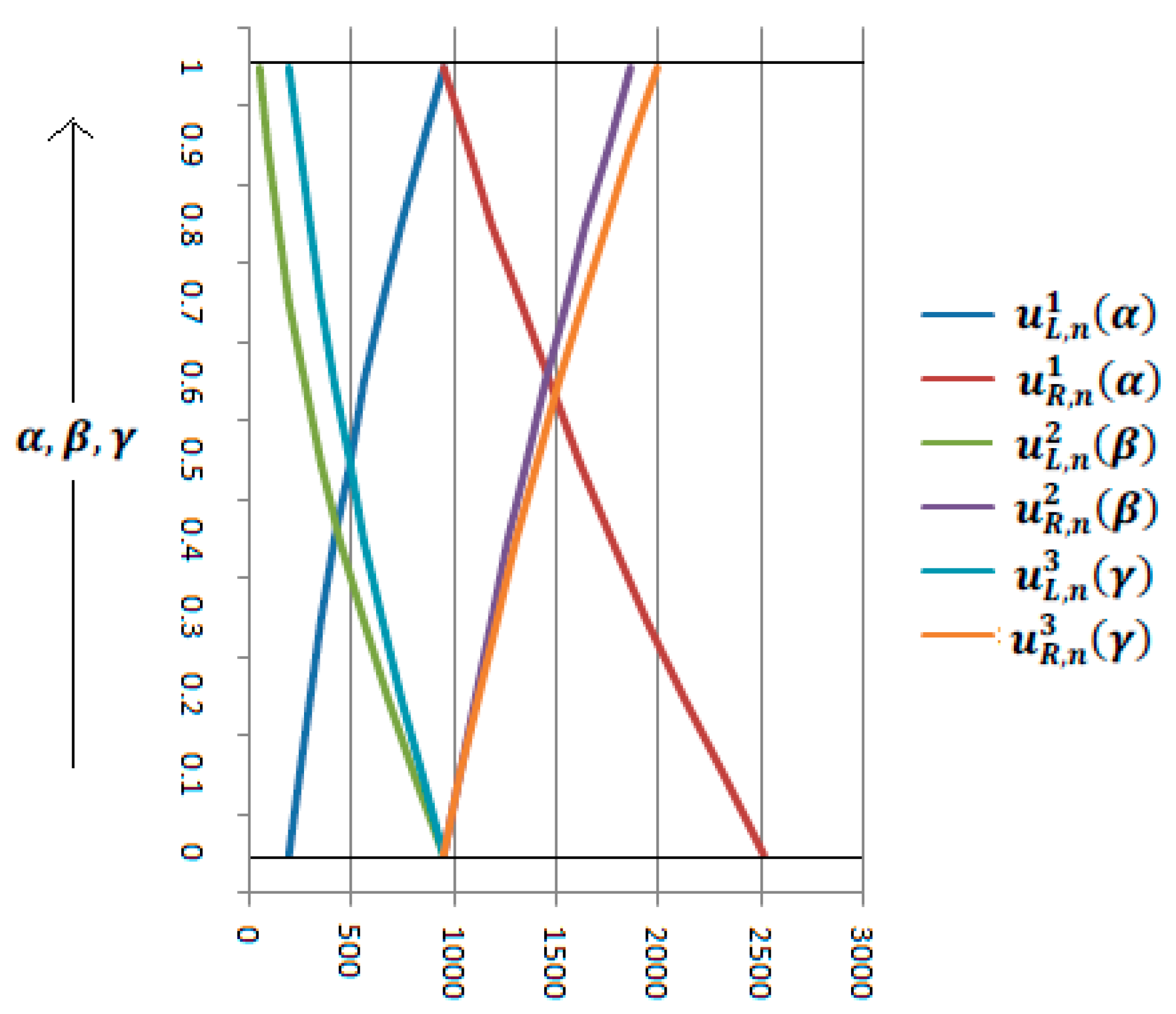
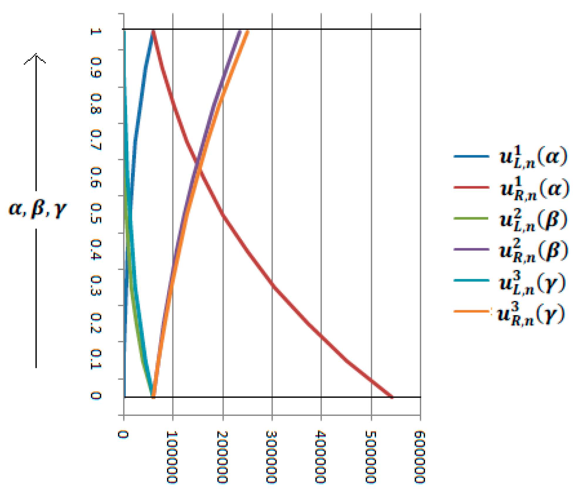
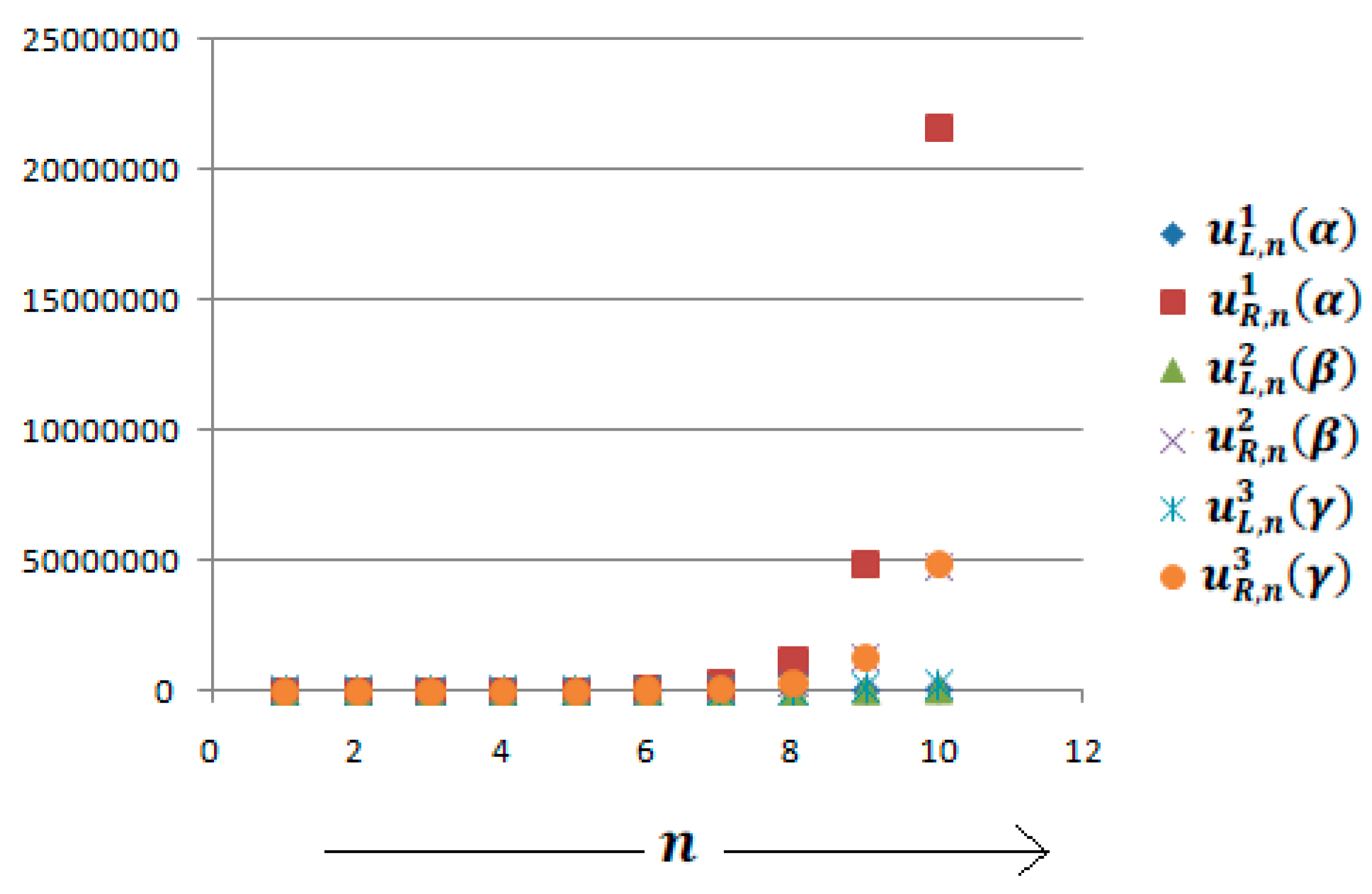
5. Numerical Example

Example 1.

Solve the difference equation:

$$u_{n+1}=\left(2,4,6;1,4,5;2,4,5\right)u_n$$

(59)

with the initial condition${\tilde{u}}_{n=0}=\left(50,60,70;55,60,75;50,60,80\right)$

Solution 1.

If the ${\left[{\tilde{u}}_n\right]}_{\left(\alpha ,\beta ,\gamma \right)}$ is the ($\alpha ,\beta ,\gamma$)-cut of a sequence of neutrosophic numbers, then its components are as follows:

$$\{\begin{array}{c}{u}_{L,n}^1\left(\alpha \right)={\left(2+2\alpha \right)}^n\left(50+10\alpha \right)\\ \begin{array}{c}{u}_{R,n}^1\left(\alpha \right)={\left(6-2\alpha \right)}^n\left(70-10\alpha \right)\\ u_{L,n}^2\left(\beta \right)={\left(4-3\beta \right)}^n\left(60-5\beta \right)\\ u_{R,n}^2\left(\beta \right)={\left(4+\beta \right)}^n\left(60+15\beta \right)\end{array}\\ u_{L,n}^3\left(\gamma \right)={\left(4-2\gamma \right)}^n\left(60-10\gamma \right)\\ u_{R,n}^3\left(\gamma \right)={\left(4+\gamma \right)}^n\left(60+20\gamma \right)\end{array}$$

(60)

Remarks 2.

We plot the solution for $\mathrm{n}=2$. From the above

Table 2. Solution for $n=2$.

$$\mathit{\alpha },\mathit{\beta },\mathit{\gamma }$$	$${\mathit{u}}_{\mathit{L},\mathit{n}}^1\left(\mathit{\alpha }\right)$$	$${\mathit{u}}_{\mathit{R},\mathit{n}}^1\left(\mathit{\alpha }\right)$$	$${\mathit{u}}_{\mathit{L},\mathit{n}}^2\left(\mathit{\beta }\right)$$	$${\mathit{u}}_{\mathit{R},\mathit{n}}^2\left(\mathit{\beta }\right)$$	$${\mathit{u}}_{\mathit{L},\mathit{n}}^3\left(\mathit{\gamma }\right)$$	$${\mathit{u}}_{\mathit{R},\mathit{n}}^3\left(\mathit{\gamma }\right)$$
0	200.00	2520.00	960.00	960.00	960.00	960.00
0.1	246.84	2321.16	814.55	1033.81	851.96	1042.22
0.2	299.52	2132.48	682.04	1111.32	751.68	1128.96
0.3	358.28	1953.72	562.18	1192.60	658.92	1220.34
0.4	423.36	1784.64	454.72	1277.76	573.44	1316.48
0.5	495.00	1625.00	359.37	1366.87	495.00	1417.50
0.6	573.44	1474.56	275.88	1460.04	423.36	1523.52
0.7	658.92	1333.08	203.96	1557.34	358.28	1634.66
0.8	751.68	1200.32	143.36	1658.88	299.52	1751.04
0.9	851.96	1076.04	93.79	1764.73	246.84	1872.78
1	960.00	960.00	55.00	1875.00	200.00	2000.00

and Figure 1, we see that ${\mathrm{u}}_{\mathrm{L},\mathrm{n}}^1\left(\mathsf{\alpha }\right)$ is an increasing function and ${\mathrm{u}}_{\mathrm{R},\mathrm{n}}^1\left(\mathsf{\alpha }\right)$ is a decreasing function, with respect to $\mathsf{\alpha }$. On the other hand, ${\mathrm{u}}_{\mathrm{L},\mathrm{n}}^2\left(\mathsf{\beta }\right)$ is a decreasing function and ${\mathrm{u}}_{\mathrm{R},\mathrm{n}}^2\left(\mathsf{\beta }\right)$ is an increasing function, with respect to $\mathsf{\beta }$. Additionally, ${\mathrm{u}}_{\mathrm{L},\mathrm{n}}^3\left(\mathsf{\gamma }\right)$ is a decreasing function and ${\mathrm{u}}_{\mathrm{R},\mathrm{n}}^3\left(\mathsf{\gamma }\right)$ is an increasing function, with respect to $\mathsf{\gamma }$. Therefore, using the concept of Definition 3.2, we call the solution a strong solution.

Remarks 3.

We plotted the solution for $\mathrm{n}=5$. From the above

Table 3. Solution for $n=5$.

$$\mathit{\alpha },\mathit{\beta },\mathit{\gamma }$$	$${\mathit{u}}_{\mathit{L},\mathit{n}}^1\left(\mathit{\alpha }\right)$$	$${\mathit{u}}_{\mathit{R},\mathit{n}}^1\left(\mathit{\alpha }\right)$$	$${\mathit{u}}_{\mathit{L},\mathit{n}}^2\left(\mathit{\beta }\right)$$	$${\mathit{u}}_{\mathit{R},\mathit{n}}^2\left(\mathit{\beta }\right)$$	$${\mathit{u}}_{\mathit{L},\mathit{n}}^3\left(\mathit{\gamma }\right)$$	$${\mathit{u}}_{\mathit{R},\mathit{n}}^3\left(\mathit{\gamma }\right)$$
0	1600.00	544,320.00	61,440.00	61,440.00	61,440.00	61,440.00
0.1	2628.35	452,886.16	41,259.65	71,251.56	46,748.74	71,830.84
0.2	4140.56	374,497.60	26,806.90	82,335.47	35,070.38	83,642.38
0.3	6297.12	307,640.56	16,748.05	94,820.44	25,898.19	97,025.57
0.4	9293.59	250,934.66	9982.01	108,844.70	18,790.48	112,143.03
0.5	13,365.00	203,125.00	5615.23	124,556.48	13,365.00	129,169.68
0.6	18,790.48	163,074.53	2937.57	142,114.45	9293.59	148,293.34
0.7	25,898.19	129,756.67	1398.99	161,688.22	6297.12	169,715.30
0.8	35,070.38	102,248.05	587.20	183,458.85	4140.56	193,651.01
0.9	46,748.74	79,721.65	206.06	207,619.30	2628.35	220,330.69
1	61,440.00	61,440.00	55.00	234,375.00	1600.00	250,000.00

and Figure 2, we see that ${\mathrm{u}}_{\mathrm{L},\mathrm{n}}^1\left(\mathsf{\alpha }\right)$ is an increasing function and ${\mathrm{u}}_{\mathrm{R},\mathrm{n}}^1\left(\mathsf{\alpha }\right)$ is a decreasing function, with respect to $\mathsf{\alpha }$. On the other hand, ${\mathrm{u}}_{\mathrm{L},\mathrm{n}}^2\left(\mathsf{\beta }\right)$ is a decreasing function and ${\mathrm{u}}_{\mathrm{R},\mathrm{n}}^2\left(\mathsf{\beta }\right)$ is an increasing function, with respect to $\mathsf{\beta }$. Additionally, ${\mathrm{u}}_{\mathrm{L},\mathrm{n}}^3\left(\mathsf{\gamma }\right)$ is a decreasing function and ${\mathrm{u}}_{\mathrm{R},\mathrm{n}}^3\left(\mathsf{\gamma }\right)$ is an increasing function, with respect to $\mathsf{\gamma }$. Therefore, using the concept of Definition 6, we call the solution a strong solution.

We interpret the solution for fixed $\alpha ,\beta ,\gamma =0.4$ and different $n$ in

Table 4. Solution for $\alpha ,\beta ,\gamma =0.4$ and different $n$.

$$\mathit{n}$$	$${\mathit{u}}_{\mathit{L},\mathit{n}}^1\left(\mathit{\alpha }\right)$$	$${\mathit{u}}_{\mathit{R},\mathit{n}}^1\left(\mathit{\alpha }\right)$$	$${\mathit{u}}_{\mathit{L},\mathit{n}}^2\left(\mathit{\beta }\right)$$	$${\mathit{u}}_{\mathit{R},\mathit{n}}^2\left(\mathit{\beta }\right)$$	$${\mathit{u}}_{\mathit{L},\mathit{n}}^3\left(\mathit{\gamma }\right)$$	$${\mathit{u}}_{\mathit{R},\mathit{n}}^3\left(\mathit{\gamma }\right)$$
1	151.20	343.20	162.40	290.40	179.20	299.20
2	381.93	1513.38	410.23	1101.80	510.47	1135.19
3	964.79	6673.49	1036.26	4180.33	1454.14	4307.01
4	2437.12	29,427.69	2617.65	15,860.57	4142.31	16,341.19
5	6156.31	129,765.52	6612.33	60,176.40	11,799.88	61,999.93
6	15,551.16	572,219.06	16,703.10	228,314.58	33,613.43	235,233.20
7	39,283.04	2,523,279.35	42,192.90	866,245.64	95,752.00	892,495.51
8	99,231.00	11,126,750.35	106,581.44	3,286,612.28	272,761.37	3,386,206.59
9	250,662.64	49,064,949.17	269,230.24	12,469,696.48	776,994.32	12,847,566.07
10	633,186.78	216,358,699.65	680,089.51	47,311,126.78	2,213,363.93	48,744,797.29

and Figure 3.

Example 2.

Solve the difference equation:

$$u_{n+1}-4u_n=0$$

(61)

with initial condition${\tilde{u}}_{n=0}=\left(50,60,70;55,60,75;50,60,80\right)$

Solution 2.

If ${\left[{\tilde{u}}_n\right]}_{\left(\alpha ,\beta ,\gamma \right)}$ is the ($\alpha ,\beta ,\gamma$)-cut of a sequence of neutrosophic numbers, then it’s components are as follows:

when $n$ is even:

$$\{\begin{array}{c}{u}_{L,n}^1\left(\alpha \right)=4^n\left(50+10\alpha \right)\\ \begin{array}{c}{u}_{R,n}^1\left(\alpha \right)=4^n\left(70-10\alpha \right)\\ u_{L,n}^1\left(\beta \right)=4^n\left(60-5\beta \right)\\ u_{R,n}^1\left(\beta \right)=4^n\left(60+15\beta \right)\end{array}\\ \begin{array}{c}{u}_{L,n}^1\left(\gamma \right)=4^n\left(60-10\gamma \right)\\ u_{R,n}^1\left(\gamma \right)=4^n\left(60+20\gamma \right)\end{array}\end{array}$$

(62)

when $n$ is odd:

$$\{\begin{array}{c}{u}_{L,n}^1\left(\alpha \right)=4^n\left(70-10\alpha \right)\\ \begin{array}{c}{u}_{R,n}^1\left(\alpha \right)=4^n\left(50+10\alpha \right)\\ u_{L,n}^1\left(\beta \right)=4^n\left(60+15\beta \right)\\ u_{R,n}^1\left(\beta \right)=4^n\left(60-5\beta \right)\end{array}\\ \begin{array}{c}{u}_{L,n}^1\left(\gamma \right)=4^n\left(60+20\gamma \right)\\ u_{R,n}^1\left(\gamma \right)=4^n\left(60-10\gamma \right)\end{array}\end{array}$$

(63)

As previous examples, we easily interpret the solutions in a different manner.

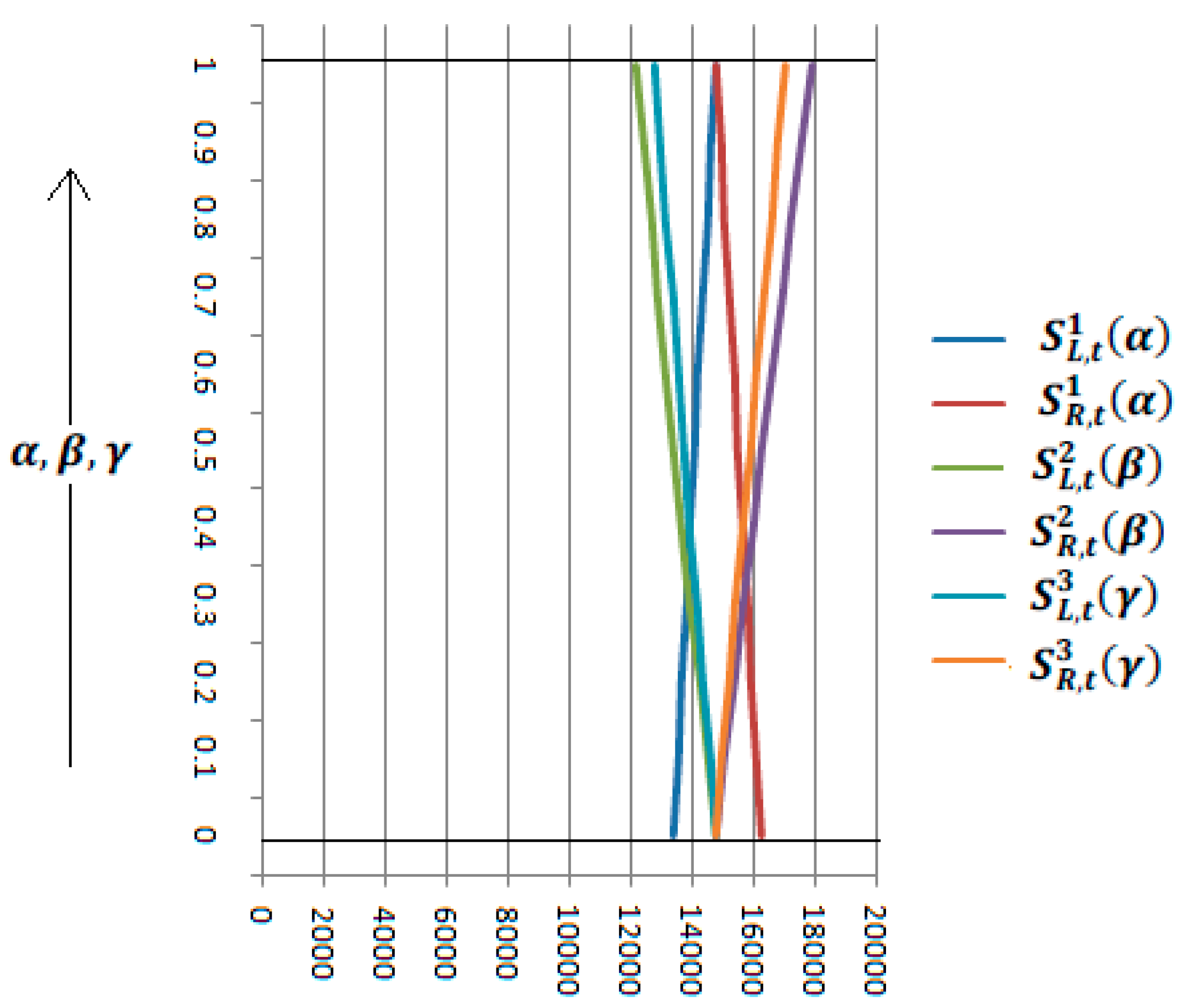
6. Application of the Method in Actuarial Science

Let us consider that a sum $S_0$ is invested at a compound interest of $i$ per unit amount and per unit of time and $S_t$ is the amount at the end of time $t$. We then get the difference equation associated with the problem, which is:

$$S_{t+1}=S_t+i{S}_t=\left(1+i\right)S_t$$

(64)

If, for some reason, $i$ may vary, we are interested to find the possible amount after a certain time interval.

For this problem, let us consider hypothetical data and solve it. Suppose a person has initially invested $S_{t=0}=10000\$$ in a firm, where they get about $4\%$ interest (which may be considered a neutrosophic value).

As per Table 1, if we take the verbal phrase for a triangular neutrosophic number, we then set the interest rate as follows:

• For the truth part: low as 3%, medium as 4%, high as 5%;
• For the falsity portion: very low as 2%, medium as 4%, very high as 6%;
• For the indeterminacy part: between low and very low 2.5%, medium 4%, between high and very high 5.5%,

i.e., we can take $\tilde{i}=\left(3,4,5;2,4,6;2.5,4,5.5\right)\%$ per annum rate. We wish to predict the amount of money after 10 years.

Therefore, we get the fuzzy difference equation

$$S_{t+1}=S_t+i{S}_t=\left(1+\tilde{i}\right)S_t$$

(65)

With the initial conditions $S_{t=0}=10000\$$ and $\tilde{i}=\left(3,4,5;2,4,6;2.5,4,5.5\right)\%$.

Solution 3.

Equation (65) is equivalent to

$$S_{t+1}=S_t+i{S}_t=\left(1+\left(0.03,0.04,0.05;0.02,0.04,0.06;0.025,0.04,0.055\right)\right)S_t$$

or

$$S_{t+1}=\left(1.03,1.04,1.05;1.02,1.04,1.06;1.025,1.04,1.055\right)S_t$$

(66)

with the initial condition $S_{t=0}=10000\$$.

The solution of (66) can be written using the concept of (19), as follows:

$$\{\begin{array}{c}{S}_{L,t}^1\left(\alpha \right)=10000{\left(1.03+0.01\alpha \right)}^t\\ \begin{array}{c}{S}_{R,t}^1\left(\alpha \right)=10000{\left(1.05-0.01\alpha \right)}^t\\ S_{L,t}^2\left(\beta \right)=10000{\left(1.04-0.02\beta \right)}^t\\ S_{R,t}^2\left(\beta \right)=10000{\left(1.04+0.02\beta \right)}^t\end{array}\\ \begin{array}{c}{S}_{L,t}^3\left(\gamma \right)=10000{\left(1.04-0.015\gamma \right)}^t\\ S_{R,t}^3\left(\gamma \right)=10000{\left(1.04+0.015\gamma \right)}^t\end{array}\end{array}$$

(67)

Remarks 4.

(1) We plot the solution for $\mathrm{t}=10$. From the above

Table 5. Solution for $t=10$.

$$\mathit{\alpha },\mathit{\beta },\mathit{\gamma }$$	$${\mathit{S}}_{\mathit{L},\mathit{t}}^1\left(\mathit{\alpha }\right)$$	$${\mathit{S}}_{\mathit{R},\mathit{t}}^1\left(\mathit{\alpha }\right)$$	$${\mathit{S}}_{\mathit{L},\mathit{t}}^2\left(\mathit{\beta }\right)$$	$${\mathit{S}}_{\mathit{R},\mathit{t}}^2\left(\mathit{\beta }\right)$$	$${\mathit{S}}_{\mathit{L},\mathit{t}}^3\left(\mathit{\gamma }\right)$$	$${\mathit{S}}_{\mathit{R},\mathit{t}}^3\left(\mathit{\gamma }\right)$$
0	13,439.1638	16,288.9463	14,802.4428	14,802.4428	14,802.4428	14,802.4428
0.1	13,570.2126	16,134.4766	14,520.2313	15,089.5813	14,590.3264	15,017.3306
0.2	13,702.4105	15,981.3266	14,242.8714	15,381.7230	14,380.9496	15,235.0219
0.3	13,835.7662	15,829.4861	13,970.2889	15,678.9453	14,174.2808	15,455.5492
0.4	13,970.2889	15,678.9453	13,702.4105	15,981.3266	13,970.2889	15,678.9453
0.5	14,105.9876	15,529.6942	13,439.1638	16,288.9463	13,768.9430	15,905.2433
0.6	14,242.8714	15,381.7230	13,180.4776	16,601.8849	13,570.2126	16,134.4766
0.7	14,380.9496	15,235.0219	12,926.2814	16,920.2240	13,374.0675	16,366.6791
0.8	14,520.2313	15,089.5813	12,676.5060	17,244.0464	13,180.4776	16,601.8849
0.9	14,660.7259	14,945.3915	12,431.0828	17,573.4357	12,989.4133	16,840.1284
1	14,802.4428	14,802.4428	12,189.9442	17,908.4770	12,800.8454	17,081.4446

and Figure 4, we see that ${\mathrm{S}}_{\mathrm{L},\mathrm{n}}^1\left(\mathsf{\alpha }\right)$ is an increasing function and ${\mathrm{S}}_{\mathrm{R},\mathrm{n}}^1\left(\mathsf{\alpha }\right)$ is a decreasing function, with respect to $\mathsf{\alpha }$. On the other hand, ${\mathrm{S}}_{\mathrm{L},\mathrm{n}}^2\left(\mathsf{\beta }\right)$ is a decreasing function and ${\mathrm{S}}_{\mathrm{R},\mathrm{n}}^2\left(\mathsf{\beta }\right)$ is an increasing function, with respect to $\mathsf{\beta }$. Additionally, ${\mathrm{S}}_{\mathrm{L},\mathrm{n}}^3\left(\mathsf{\gamma }\right)$ is a decreasing function and ${\mathrm{S}}_{\mathrm{R},\mathrm{n}}^3\left(\mathsf{\gamma }\right)$ is an increasing function, with respect to $\mathsf{\gamma }$. Therefore, using the concept of Definition 3.2, we call the solution a strong solution. (2) From Table 5, we can see that we find the crisp solution at $\mathsf{\alpha }=1$, $\mathsf{\beta },\mathsf{\gamma }=0$ (since, at $\mathsf{\alpha }=1$, $\mathsf{\beta },\mathsf{\gamma }=0,$ the neutrosophic number becomes a crisp number) and for $\mathrm{t}=10$ is equal to 14802.4428. Therefore, we can say that after 10 years, the most probable chance to get the money is 14802.4428$.(3) If we consider $\mathsf{\alpha }=0$ and $\mathsf{\beta },\mathsf{\gamma }=1$, i.e., in the case that we get the most uncertain solution interval, we observe that the truthiness of the solution belongs to the interval $\left[13439.1638,16288.9463\right]$, the falsity belongs to the interval $\left[12189.9442,17908.4770\right]$, and the indeterminacy belongs to the interval $\left[12800.8454,17081.4446\right]$.

7. Conclusions and Future Research Scope

In this paper, we find the solution strategy for solving and analyzing homogeneous linear difference equations with neutrosophic numbers, i.e., we found the solutions of the homogeneous difference equations with initial conditions and coefficients, both as neutrosophic numbers. We demonstrate the solution of different cases using the neutrosophic characterization theorem, which is established in this paper. The strong and weak solution concepts are also applied to different results.

Moreover, the outcomes of the study are as follows:

(1)

The difference type of the homogeneous difference equation is solved in a neutrosophic environment and the symmetric behavior between them is discussed.

(2)

The characterization theorem for the neutrosophic difference equations are established.

(3)

The strong and weak solution concept is applied for the neutrosophic difference equation.

(4)

Different examples and real-life applications in actuarial science are illustrated for better understanding of neutrosophic difference equations.

For some limitations, we did not study the different perspectives of related research in the theory of difference equations with uncertainty in this present work. From this work, anyone can take motivation and find a new theory and results in the following field, as follows:

(1)

The solution of difference equation can be found with different types of uncertainty, such as Type 2 fuzzy, interval valued fuzzy, hesitant fuzzy, rough fuzzy environment.

(2)

Finding several methods (analytical and numerical) for solving non-linear first and higher order difference equations or system of difference equations with uncertainty.

(3)

Solving the real-life model associated with the discrete system modeling with uncertain data.

As a final argument, we can surely say that this research is very helpful to the research community who deals with discrete system modeling with uncertainty.

References

1. Zadeh, L. Fuzzy sets. Inf. Control. 1965, 8, 338–353. [Google Scholar] [CrossRef] [Green Version]
2. Atanassov, K.T. Intuitionistic fuzzy sets. Fuzzy Sets Syst. 1986, 20, 87–96. [Google Scholar] [CrossRef]
3. Li, J.; Niu, Q.; Dong, X.-C. Similarity Measure and Fuzzy Entropy of Fuzzy Number Intuitionistic Fuzzy Sets. Adv. Intell. Soft Comput. 2009, 54, 373–379. [Google Scholar] [CrossRef]
4. Ye, J. Prioritized aggregation operators of trapezoidal intuitionistic fuzzy sets and their application to multicriteria decision-making. Neural Comput. Appl. 2014, 25, 1447–1454. [Google Scholar] [CrossRef]
5. Smarandache, F. A Unifying Field in Logics Neutrosophy: Neutrosophic Probability, Set and Logic; American Research Press: Rehoboth, DE, USA, 1998. [Google Scholar]
6. Wang, H.; Smarandache, F.; Zhang, Y.; Sunderraman, R. Single Valued Neutrosophic Sets. Multisspace Multistructure 2010, 4, 410–413. [Google Scholar]
7. Ye, J. Single-Valued Neutrosophic Minimum Spanning Tree and Its Clustering Method. J. Intell. Syst. 2014, 23, 311–324. [Google Scholar] [CrossRef] [Green Version]
8. Peng, J.-J.; Wang, J.-Q.; Wang, J.; Zhang, H.-Y.; Chen, X.-H. Simplified neutrosophic sets and their applications in multi-criteria group decision-making problems. Int. J. Syst. Sci. 2015, 47, 1–17. [Google Scholar] [CrossRef]
9. Peng, X.; Smarandache, F. New multiparametric similarity measure for neutrosophic set with big data industry evaluation. Artif. Intell. Rev. 2019, 53, 3089–3125. [Google Scholar] [CrossRef]
10. Chakraborty, A.; Mondal, S.P.; Ahmadian, A.; Senu, N.; Salahshour, S.; Alam, S. Different Forms of Triangular Neutrosophic Numbers, De-Neutrosophication Techniques, and their Applications. Symmetry 2018, 10, 327. [Google Scholar] [CrossRef] [Green Version]
11. Chakraborty, A.; Mondal, S.P.; Alam, S.; Ahmadian, A.; Senu, N.; De, D.; Salahshour, S. Disjunctive Representation of Triangular Bipolar Neutrosophic Numbers, De-Bipolarization Technique and Application in Multi-Criteria Decision-Making Problems. Symmetry 2019, 11, 932. [Google Scholar] [CrossRef] [Green Version]
12. Deli, I.; Ali, M.; Smarandache, F. Bipolar Neutrosophic Sets and their Application Based on Multi-Criteria Decision Making Problems. In Proceedings of the 2015 International Conference on Advanced Mechatronic Systems (ICAMechS), Beijing, China, 22–24 August 2015; Institute of Electrical and Electronics Engineers (IEEE): Piscataway, NJ, USA, 2015; pp. 249–254. [Google Scholar]
13. Lee, K.M. Bipolar-Valued Fuzzy Sets and their Operations. In Proceedings of the International Conference on Intelligent Technologies, Bangkok, Thailand, 12–14 December 2000; pp. 307–312. [Google Scholar]
14. Kang, M.K.; Kang, J.G. Bipolar fuzzy set theory applied to sub-semigroups with operators in semi groups. J. Korean Soc. Math. Educ. Ser. B Pure Appl. Math. 2012, 19, 23–35. [Google Scholar]
15. Smarandache, F. Neutrosophic Perspectives: Triplets, Duplets, Multisets, Hybrid Operators, Modal Logic, Hedge Algebras and Applications; Degree of Dependence and Independence of the (Sub) Components of Fuzzy Set and Neutrosophic Set. Neutrosophic Sets and Systems; Pons Publishing House: Stuttgart, Germany, 2016; Volume 11, pp. 95–97. [Google Scholar]
16. Deeba, E.Y.; De Korvin, A.; Koh, E.L. A fuzzy difference equation with an application. J. Differ. Equ. Appl. 1996, 2, 365–374. [Google Scholar] [CrossRef]
17. Deeba, E.; De Korvin, A. Analysis by fuzzy difference equations of a model of CO2 level in the blood. Appl. Math. Lett. 1999, 12, 33–40. [Google Scholar] [CrossRef] [Green Version]
18. Lakshmikantham, V.; Vatsala, A. Basic Theory of Fuzzy Difference Equations. J. Differ. Equ. Appl. 2002, 8, 957–968. [Google Scholar] [CrossRef]
19. Papaschinopoulos, G.; Papadopoulos, B.K. On the fuzzy difference equation x_(n+1)=A+B⁄x_n. Soft Comput. 2002, 6, 456–461. [Google Scholar] [CrossRef]
20. Papaschinopoulos, G.; Papadopoulos, B.K. On the fuzzy difference equation x_(n+1)=A+x_n⁄x_(n-m). Fuzzy Sets Syst. 2002, 129, 73–81. [Google Scholar] [CrossRef]
21. Papaschinopoulos, G.; Schinas, C.J. On the fuzzy difference equation x n + 1 k = 0 k = 1 A i x n i p i + 1 x n k p k . J. Differ. Equ. Appl. 2000, 6, 85–89. [Google Scholar] [CrossRef]
22. Papaschinopoulos, G.; Stefanidou, G. Boundedness and asymptotic behavior of the solutions of a fuzzy difference equation. Fuzzy Sets Syst. 2003, 140, 523–539. [Google Scholar] [CrossRef]
23. Umekkan, S.A.; Can, E.; Bayrak, M.A. Fuzzy difference equation in finance. IJSIMR 2014, 2, 729–735. [Google Scholar]
24. Stefanidou, G.; Papaschinopoulosand, G.; Schinas, C.J. On an exponential–Type fuzzy Difference equation. Advanced in difference equations. Adv. Differ. Equ. 2010, 2010, 1–19. [Google Scholar] [CrossRef] [Green Version]
25. Din, Q. Asymptotic Behavior of a Second-Order Fuzzy Rational Difference Equation. J. Discret. Math. 2015, 2015, 1–7. [Google Scholar] [CrossRef]
26. Zhang, Q.H.; Yang, L.H.; Liao, D.X. Behaviour of solutions of to a fuzzy nonlinear difference equation. Iran. J. Fuzzy Syst. 2012, 9, 1–12. [Google Scholar]
27. Memarbashi, R.; Ghasemabadi, A. Fuzzy difference equations of volterra type. Int. J. Nonlinear Anal. Appl. 2013, 4, 74–78. [Google Scholar]
28. Stefanidou, G.; Papaschinopoulos, G. A fuzzy difference equation of a rational form. J. Nonlinear Math. Phys. 2005, 12, 300–315. [Google Scholar] [CrossRef] [Green Version]
29. Chrysafis, K.A.; Papadopoulos, B.K.; Papaschinopoulos, G. On the fuzzy difference equations of finance. Fuzzy Sets Syst. 2008, 159, 3259–3270. [Google Scholar] [CrossRef]
30. Mondal, S.P.; Vishwakarma, D.K.; Saha, A.K. Solution of second order linear fuzzy difference equation by Lagrange’s multiplier method. J. Soft Comput. Appl. 2016, 2016, 11–27. [Google Scholar] [CrossRef] [Green Version]
31. Mondal, S.P.; Mandal, M.; Bhattacharya, D. Non-linear interval-valued fuzzy numbers and their application in difference equations. Granul. Comput. 2017, 3, 177–189. [Google Scholar] [CrossRef]
32. Sarkar, B.; Mondal, S.P.; Hur, S.; Ahmadian, A.; Salahshour, S.; Guchhait, R.; Iqbal, M.W. An optimization technique for national income determination model with stability analysis of differential equation in discrete and continuous process under the uncertain environment. Rairo Oper. Res. 2019, 53, 1649–1674. [Google Scholar] [CrossRef] [Green Version]
33. Zhang, Q.; Lin, F. On Dynamical Behavior of Discrete Time Fuzzy Logistic Equation. Discret. Dyn. Nat. Soc. 2018, 2018, 1–8. [Google Scholar] [CrossRef]
34. Zhang, Q.; Lin, F.; Zhong, X. Asymptotic Behavior of Discrete Time Fuzzy Single Species Model. Discret. Dyn. Nat. Soc. 2019, 2019, 1–9. [Google Scholar] [CrossRef]
35. Zhang, Q.; Lin, F.B.; Zhong, X.Y. On discrete time Beverton-Holt population model with fuzzy environment. Math. Biosci. Eng. 2019, 16, 1471–1488. [Google Scholar] [CrossRef] [PubMed]
36. Khastan, A. Fuzzy logistic difference equation. Iran. J. Fuzzy Syst. 2018, 15, 55–66. [Google Scholar]
37. Mondal, S.P.; Alam Khan, N.; Vishwakarma, D.; Saha, A.K. Existence and Stability of Difference Equation in Imprecise Environment. Nonlinear Eng. 2018, 7, 263–271. [Google Scholar] [CrossRef]
38. Khastan, A.; Alijani, Z. On the new solutions to the fuzzy difference equation xn+1=A+Bxn. Fuzzy Sets Syst. 2019, 358, 64–83. [Google Scholar] [CrossRef]
39. Khastan, A. New solutions for first order linear fuzzy difference equations. J. Comput. Appl. Math. 2017, 312, 156–166. [Google Scholar] [CrossRef]
40. Abdel-Basset, M.; Mohamed, M.; Hussien, A.N.; Sangaiah, A.K. A novel group decision-making model based on triangular neutrosophic numbers. Soft Comput. 2018, 22, 6629–6643. [Google Scholar] [CrossRef]
41. Jensen, A. Lecture Notes on Difference Equation; Department of mathematical Science, Aalborg University: Aalborg, Denmark, 18 July 2011; (It is lecture notes of the courses “Introduction to Mathematical Methods” and “Introduction to Mathematical Methods in Economics”). [Google Scholar]
42. Elaydi, S.N. An Introduction to Difference Equations; Springer: Berlin/Heidelberg, Germany, 1995. [Google Scholar]
Figure 1. Graph for n = 2 .
Symmetry 12 01091 g001
Figure 2. Graph for n = 5 .
Symmetry 12 01091 g002
Figure 3. Graph for α , β , γ = 0.4 and different n .
Symmetry 12 01091 g003
Figure 4. Graph for t = 10 .
Symmetry 12 01091 g004