Image-Level Structure Recognition Using Image Features, Templates, and Ensemble of Classifiers

Abstract

Image-level structural recognition is an important problem for many applications of computer vision such as autonomous vehicle control, scene understanding, and 3D TV. A novel method, using image features extracted by exploiting predefined templates, each associated with individual classifier, is proposed. The template that reflects the symmetric structure consisting of a number of components represents a stage—a rough structure of an image geometry. The following image features are used: a histogram of oriented gradient (HOG) features showing the overall object shape, colors representing scene information, the parameters of the Weibull distribution features, reflecting relations between image statistics and scene structure, and local binary pattern (LBP) and entropy (E) values representing texture and scene depth information. Each of the individual classifiers learns a discriminative model and their outcomes are fused together using sum rule for recognizing the global structure of an image. The proposed method achieves an 86.25% recognition accuracy on the stage dataset and a 92.58% recognition rate on the 15-scene dataset, both of which are significantly higher than the other state-of-the-art methods.

1. Introduction

A human brain can understand images of natural, urban outdoor and indoor 3D scenes efficiently [1,2]. This is because the world around us behaves regularly, and structural regularities are directly reflected in the 2D image scene [3]. These regularities are also proposed for use in machine vision systems. Nedovic et al. [4] identified several image-level 3D scene geometries on 2D images called ‘stages’. They may contain a straight background (like a wall, façade of a building, or mountain range) or a box with three sides, e.g., a corridor, tunnel, close street, etc., Figure 1 illustrates some of them. Stages are rough models of 3D scene geometry, with small objects ignored. As stages are limited, they can be used for 3D scene information extraction, e.g., for an autonomous vehicle, robot navigation system, or scene understanding. In the literature, Nedovic et al. [4] and Lou et al. [5] introduce stage recognition algorithms by using low-level feature sets and these features are combined at each local region. Lou et al. [5] use predefined template-based segmentation to extract features, namely histograms of oriented gradients (HOGs) [6], mean color values (Hue, Saturation and Value (HSV) and red (R), green(G), and blue(B)), and parameters of Weibull distribution features [7] for each image patch and introduced a graphical model to learn mapping from image features to a stage. Other approaches to scene recognition are based on Bag of Words (BoW) models [8], e.g., J. Sánchez et al. [9] use dense Scale-invariant feature transform (SIFT) features in the Fisher Kernel framework as an alternative patch encoding strategy and obtain reasonable accuracy.

The most recent approaches of image recognition are based on convolutional neural networks (CNN). The CNN and other ‘deep networks’ are generally trained on large datasets, e.g., ImageNet [10], and Places365 [11], and have achieved high-performance on many applications such as image classification, face recognition, and object detection [11,12,13,14,15]. The large annotated dataset required by certain models is a particular problem, which is one of CNNs’ main challenges. Other CNN challenges include the fact that they require high-performance hardware and hyper parameter optimization. These issues exist in an image-level structure recognition as well. The above methods suffer from intra-class variation or have complex structures. In this research work, we demonstrate a novel method of image-level structure recognition that utilizes image features and these features are extracted based on predefined templates [5], where the each template is associated with an individual classifier. The set of features, namely the histogram of oriented gradient (HOG) [6] features exhibiting overall object shapes, colors (RGB and HSV) representing scene information, the parameters of the Weibull distribution [7], features exhibiting relation between image statistics and scene structure, and, lastly, the (LBP) [16,17] and entropy (E) values (LBP-E), representing texture and scene depth information, are extracted from each local region. This means that each feature type provides different representations of an input image. In the implementation, each image is parsed into several predefined templates to obtain various segments. These template-based segments are obtained by using component of templates as initial contours in the active contour algorithm [18]. Next, the features are extracted by following template-based image segmentation to obtain the rich information of the image’s geometric structure, and we utilize these features to learn the image-level structure of scene images. Each template has a unique structure and by following this structure, the sequence of features is distinct. Therefore, each feature vector, which we obtain by using a certain template, is fed to the individual classifier. Finally, the ensemble of classifier outcomes are combined by using sum rule [19,20,21,22] to predict the image label.

The state-of-the-art methods do not share their stage datasets publicly. Thus, we construct a new stage dataset by following the 12 stages proposed in [4]. Secondly, we utilize the ‘15-scene image dataset’ introduced in [23] and its categories on the basis of a global image structure. The results of the stage dataset show that the proposed method achieves an 82.50% accuracy by using half of the dataset for training and half for testing. The state-of-the-art methods, such as the method by Sánchez et al. [9], obtain 72.40% accuracy in terms of stage recognition. Next, the experimental outcomes of the proposed method with the standard ‘15-scene image dataset’ benchmark demonstrate remarkable gains within the recognition accuracy compared to the state-of-the-art methods. The proposed method achieves superior accuracy by employing the following main contributions:

• Utilizing five different features for the study of the image-level structure recognition.
• Performing feature-level fusion for each sub-region (e.g., sky or ground) of an image and concatenating these features into a single set for a whole image.
• Using individual classifiers for each template outcome and, later on, fusing output classifiers at the decision level to predict a class label.
• Results exhibiting that the feature-level fusion and decision-level fusion approaches improve the recognition accuracy significantly.

The rest of the paper is organized as follows. Previous studies on image-level structure recognition are reviewed in Section 2. The techniques used in the proposed method are described in Section 3. Section 4 explains the proposed method. In Section 5, the explanation of the implementation, experimental descriptions and the results of the state-of-the-art methods are given. Finally, the discussion and conclusion are presented in Section 6.

2. Related Work

Torrialba and Oliva et al. [24] use local and global image scene information to represent the spatial structure of the scene. By employing the Gist descriptor, they estimate the relation between spatial properties and scene categories. Fei-Fei and Perona [25] proposed a scheme with the use of theme entities to represent the image regions and to learn the distribution of scene categories for themes. However, the number of scene categories in this scheme is very large [5]. Hoiem et al. [26] modeled a scene with three geometrical components. They trained a set of classifiers to parse the scenes into three parts: sky, vertical (background) and ground. Thus, they classified input images into three categories. This means the model can only handle the outdoor images. Other approaches of scene recognition are based on Bag of Words (BoW) models [8], e.g., that of J. Sánchez et al. [9], who obtained a reasonable accuracy of 47.2% by using 50% samples for training of the SUN dataset [27]. Similarly, Zafar et al. [23] introduced a new method based on BoW by computing an orthogonal vector histogram (OVH) for triplets of identical visual words. The histogram-based representation is computed by using the magnitude of these orthogonal vectors. This method is based on the geometric relationships among visual words and the computation complexity of these approaches increases exponentially with the increasing size of the codebook [28,29]. The methods based on BoW have improved the recognition performance, but due to the limitation of the representation capability of the BoW model, no further astonishing accuracy has been achieved for scene recognition [30]. On the other hand, the large scene datasets are mostly categorized into a very large number of classes, e.g., the SUN dataset [27] and Places365 dataset [11] have hundreds of scene classes.

Instead of considering the large number of scene categories, Nedovic et al. [4] introduce a generic approach in which scenes are categorized into a limited set of image-level 3D scene geometries. To model the scene geometries, 12 stages are introduced, such as sky–ground, sky–background–ground, and box. Nedovic et al. [4] use a uniform grid to extract the feature set, including the texture gradient, by parameters of Weibull distribution (four features), atmospheric scattering (five features), and perspective line (eight features) for stage recognition. They use the multi-class support vector machine (SVM) for stage recognition and achieve a 38.0% accuracy on a stage dataset which contains around 2000 images [4]. As the features are extracted using a uniform grid, this result in large differences within the same class if the image structure is slightly changed [5]. Lou et al. [5] use predefined template-based segments to extract the feature set namely, HOG features [6,31] (nine features), mean color value (HSV and RGB, six features), parameters of Weibull distribution [7] (four features) for each image patch and proposed a graphical model to map the image features to the output stages. They use latent variables to model possible subtopics, e.g., sky, background or ground. In consequence, Lou et al. [5] achieve a 47.30% accuracy in terms of stage recognition by utilizing the dataset [4]. In this method, the author extracts features by following the hard and soft segmentation techniques. Hard segmentation is predefined by the template and soft segmentation is obtained by using Carreira and Sminchisescu’s [32] segmentation method. This is the figure–ground segmentation method and it generates foreground segments for each seed at different scales by solving the max-flow energy optimization. Thus, for each image, it generates hundreds of segments [5] and finds the segment that has the largest overlap-to-union score for each component of the templates, which is computationally expensive.

Recently, CNNs have revolutionized computer vision, being the catalysts for significant performance gains in many applications such as scene classifications [11], texture recognition, and facial applications [33], etc. CNN-based methods consist of several convolution layers and pooling operations accompanied by one or more fully connected (FC) layers. The popular CNN architectures, such as GoogLeNet [12], ResNet [13], AlexNet [14], and VGG-16 [15] are generally trained on the large amount of label training data [10,11] with a fixed input size and a high performance. The classification performance of CNN-based methods depends on the dataset. Some studies such as [34,35] have claimed that replacing the FC layers of the trainable classifier (conv. Softmax function) of a deep CNN model with a linear Support Vector Machine (SVM) can improve the classification performance, as it achieves 99.04% accuracy on a handwritten dataset [36].

Moreover, CNNs require large datasets for training and collecting a large annotated dataset for a specific problem is a one of the CNN main challenges. Consequently, the representation of indoor and outdoor images into image-level structures is limited, and the problem is more tractable. Thus, the new method of image-level structure recognition proves that utilizing feature-level fusion by following template-based segmentations and the decision-level fusion of an ensemble of classifiers, where each classifier is associated with the rough structure/template, are beneficial for image-level structure recognition and offer significant improvements in recognition accuracy.

3. Background

Image features (HOG, colors, Weibull parameters, LBP-E) are introduced in Section 3.1. Section 3.2 introduces the templates and template-based segmentation. Section 3.3 illustrates the classifier, the ensemble of classifiers, and their performance measurements.

3.1. Image Features

3.1.1. Parameters of Weibull Distribution

The relation between scene depth and natural image statistics (e.g., texture, edges) is studied in [4,7]. Nedovic et al. [4] show that parameters of the Weibull distribution [7] can identify the local depth order and the direction of depth. Thus, the four features, parameters of Weibull distribution, $\propto$ and β are obtained for the x and y direction of each image patch (see at [4], Equation (2)).

3.1.2. Color Features

The properties of a light source and colors of scene objects can be used for stage classification [4]. Two different models, RGB and HSV, are used as feature sets. Red green blue (RGB) is a set of primary colors, and each color is specified by the intensity of the primary colors. The image is represented as a three-dimensional array $I\left(H, W, 3\right)$, H and W are the number of rows and columns, respectively. By following Nedovic et al. [4], the three features of the color correction coefficient of RGB are estimated by a grey world algorithm [37] and the other three features, Hue, Saturation and Value (HSV), are included in a color feature set as they show interesting behaviors in order to increase or decrease the depth of the image [4].

3.1.3. Histogram of Oriented Gradients (HOG)

It is a fact that the HOG is one of the most popular feature extractors and has been widely used in an object detection for representing the shape of objects [6,31]. In our study, its useful features for differentiating the image geometry such as the shape of the sky–ground and the shape of the corner are very different. HOG features can be calculated with the following steps: gradient computation, orientation binning, and bin vector normalization. The gradient is computed using Gaussian image smoothing followed by a discrete derivative calculation. To obtain the gradient $\partial I/\partial x$ of an image, the mask, $f$, is used as a convolutional filter on an image $I\left(x, y\right),$ by

$$\frac{\partial I(x,y)}{\partial x}=I(x,y)*f(x)={\displaystyle \sum _{i=-m}^{m}f(i)\times I(x,y+i)}$$

(1)

where $f=\left[-m,0,m\right]$, m = 1 for first derivative, ‘*’ is a convolutional operator. $\partial I/\partial x$ is a gradient for the x direction. Similarly, the gradient of vertical direction $\partial I/\partial y$ can be measured using the mask $f^{\prime }$. For RGB images, the gradients of each color channel are calculated separately, and the one with the largest norm is taken as the pixel gradient. In the next step, the linear gradient voted in through orientation binning (B) is evenly spaced over [0,180] degrees. B is initialized to nine in our implementation, as described in [6]. After obtaining a bin vector ‘V’ (with a dimension B) for a single image patch, it is normalized by its ‘L2- norm’, given by

$$V\leftarrow \frac{V}{\sqrt{\Vert V{\Vert }_2^2+{\epsilon }^2}}$$

(2)

where $\epsilon$ is a small constant to avoid the undefined value. It is equal to $0.01$ to minimize its influence on HOG features.

3.1.4. Local Binary Pattern and Entropy Value (LBP-E)

One of the most successful approaches for texture description is a local binary pattern (LBP) and its variants [16]. LBP features describe the neighborhood of a pixel by its binary derivatives (differences in a central pixel with its neighborhood). These binary derivatives are used to form a small code to describe the neighborhood of the pixel. The LBP code describing the local image texture around the center pixel, $\left(x_c,y_c\right)$, of the radius, $R$, with $P$ points is computed as:

$$LB{P}_{P,R}(x_c,y_c)={\displaystyle \sum _{i=0}^{P-1}t(I(x_i,y_i)}-I(x_c,y_c))\times 2^i$$

(3)

where the threshold function is defined as:

$$t(k)=\{\begin{array}{l}0,\begin{array}{cc}for& k\end{array}<0\\ 1,\begin{array}{cc}for& k\end{array}\ge 0.\end{array}$$

(4)

In the case of an 8-pixel neighborhood, $P=8$, the LBP code is in the range from zero to 255.

The LBP features are obtained by computing the normalized histogram with n bins of LBP codes over each image patch.

Entropy (E) is another simple approach to describe texture content. It is a function which measures the variability of a data [38]. It provides depth information, which can be used to classify the stages such as the entropy value of the sky is very different from the entropy value of the ground region. E is computed for the LBP histogram, and we obtain a single E value for each image patch. For the implementation, we use n = 5 bins of LBP code histograms to capture the generic information for each patch. Thus, the LBP-E provides six features for each image patch.

Note that graphical representation of relationship of image depth and features (parameters of Weibull distribution, color and LBP-E) are given in Supplementary Material, Figures S1–S4.

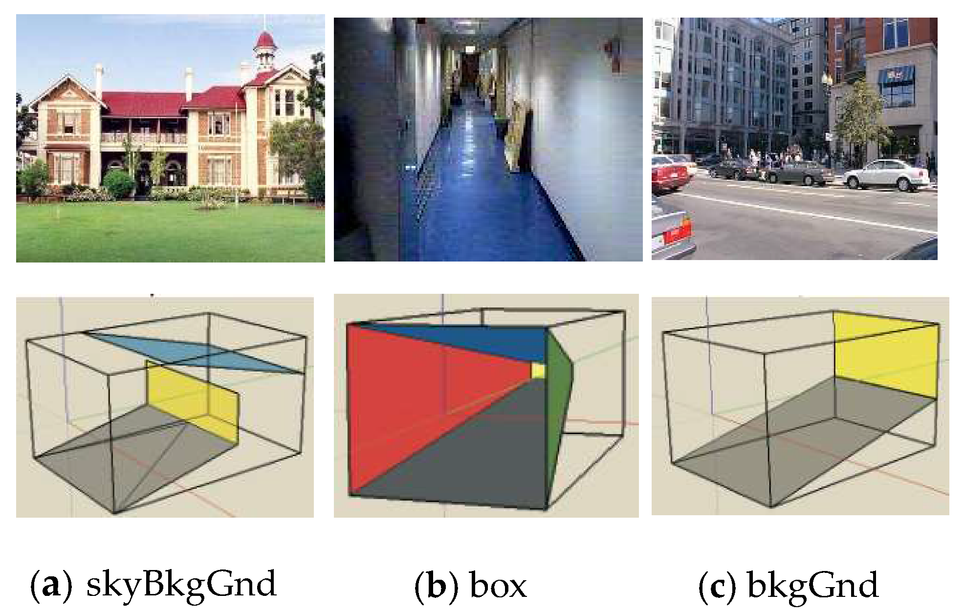
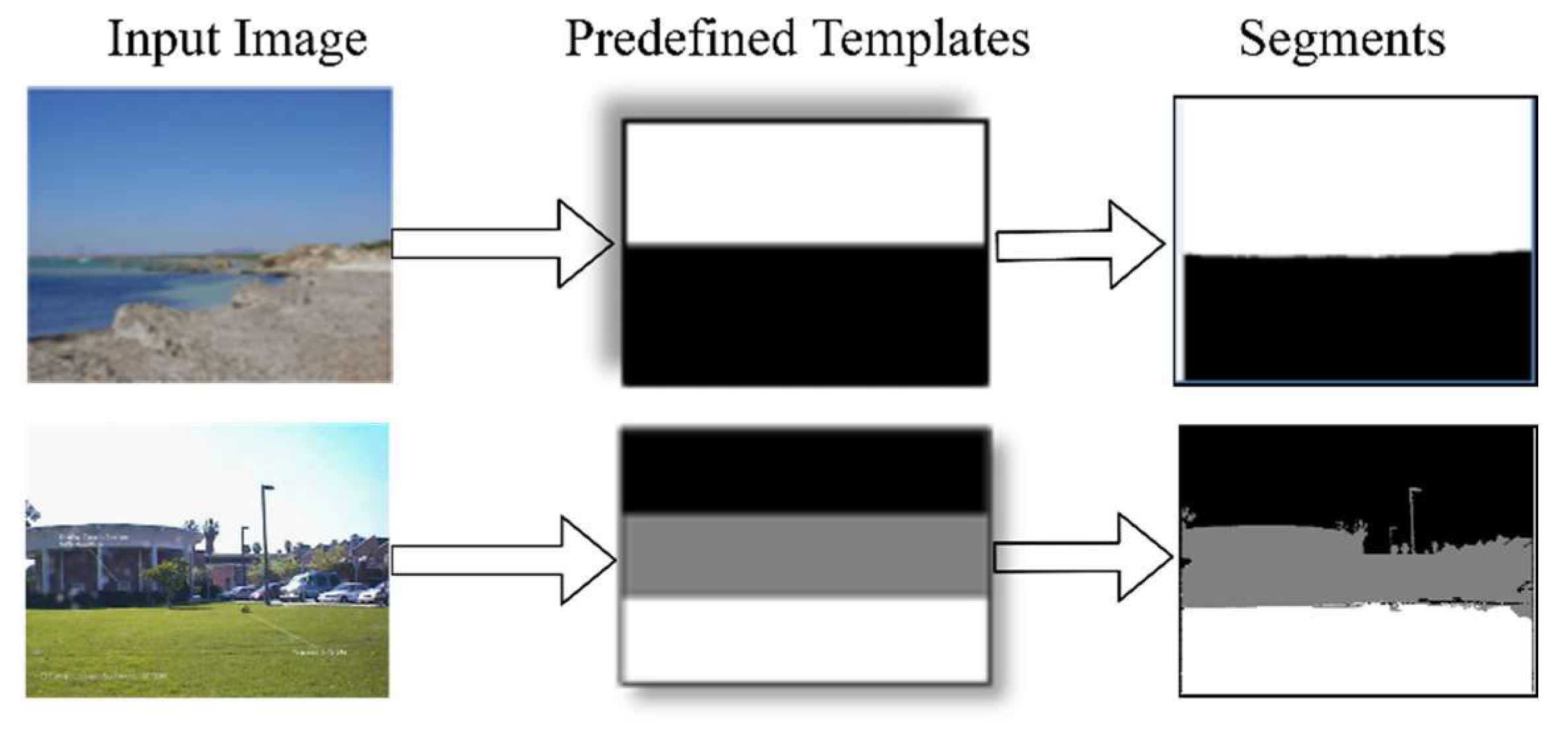
3.2. Template-Based Segmentation

The predefined template which reflects to the symmetric structure, represents a 2D rough structure of a 3D scene geometry [5]. The template is defined as follows: a template T, has the same size $H\times W$ as the input image I. It is composed of S segments ${\mathrm{s}}_k, k=1,\dots ,S$. Element $T_i{}_j=k$, if pixel $I\left(i,j\right)$ belongs to the segment $s_k$, e.g., in Figure 2a,c,d, the templates have two components ($S=2$) and templates in Figure 2b,g,h have three components ($S=3$). Template (f) indicates the whole image as a one segment.

Lou et al. [5] use soft and hard segmentation. Hard segmentation is predefined by the template, but the method of hard segmentation is not explicitly defined. Soft segmentation is based on the figure–ground segmentation method proposed by Carrira and Sminchinsescu [32]. Foreground seeds are uniformly placed on a grid, and the background seeds are placed on the borders of the image. This generates several segments from each seed at different scales by solving the max-flow energy optimization. In this way, hundreds of segments generate for each image and they select the segment that has the largest overlap-to-union score for a component of the templates. For each component, the algorithm then needs to find the best fitting segment and this is computationally expensive. Instead of using both hard and soft segmentation, the active contours algorithm [18] generates an accurate segment if a component of the templates is used as an initial contour. The active contours algorithm is a segmentation technique that uses energy constraints and forces within the image for the separation of the region of interest. It separates the boundaries of the regions of target objects for segmentation. The region of interest possesses a group of pixels such as circles, polygons or irregular shapes. In MATLAB, the interface of the aforementioned function, ‘activecontour (I, mask)’, is given. It segments the image I into foreground and background regions using active contours. The mask indicates the initial contours (e.g., a component of the template) for a particular image.

3.3. Classifier, Ensemble of Classifiers, and Their Performance Measures

After the features have been determined, a classifier is required to map these features into the limited classes. A classifier can be defined as a pattern recognition technique that categorizes a huge number of data into limited classes [39]. A mathematical model is required that it is powerful enough to discern all given classes and thus resolve the recognition task. Determining a given classifier’s parameters is a typical learning problem, and thus is affected by the problems concerning this field. An output of a classifier can be represented as a score vector where the dimension of the vector is equal to the number of classes [20,21,40]. A probabilistic classifier generates an output of probability distribution over a set of classes with elements belonging to [0,1].

An ensemble of classifiers increase the performance of pattern recognition applications [19,20,21,22]. Typical ensembles of classifiers use outputs from individual classifiers and produce a combined output for each class/stage. To fuse the outputs of classifiers, two kinds of strategies can be used: soft-level and hard-level combination [20]. Hard-level fusion uses the outputs labels of the classifiers, e.g., by majority voting. Soft-level fusion uses estimate of the a posteriori probability or score of the stage. The sum, max, product, and min rules belong to the soft-level combination. In [21,22], it is shown that the sum rule is simple and has a low error rate.

The sum rule uses the summation of the scores or a posteriori probabilities. It simply adds the scores or a posteriori probabilities, which is provided by each classifier for each stage, and derives the stage label for the input image with the maximal sum value.

In order to evaluate different methods compared to one another, the following metrics are calculated: confusion matrix [41], accuracy [5,42], mean precision [41], mean recall [41], and mean F-score value [41]. Let Ɲ denote the number of samples in a dataset. N is the number of samples used for training and M is the number of samples used for testing, Ɲ = M + N. S denotes the stages, $M_c$ represents the number of samples truly belonging to the c-th stage, while $M_c^{\prime }$ the number of samples predicted as belonging to the c-th stage. A classifier is trained on N training samples, and derives a model to predict the class types of M testing samples.

The classification results can be represented in the confusion matrix [41]. It is a square $S\times S$ matrix whose rows and columns represent true and predicted stages, respectively. Its every entry $G_{cg}$ represents the number of samples belonging to the c-th stage and predicted as belonging to the g-th stage. The diagonal elements $G_{cc}$ represent the number of correctly classified samples, while remaining elements represent the number of incorrectly classified samples. The confusion matrix contains all the information related to the distribution of samples within the stage and the classification performance. The number of test samples M are:

$$M={\displaystyle \sum _{c=1}^S{\displaystyle \sum _{g=1}^S{G}_{cg}}}$$

(5)

The number of samples truly belonging to the c-th stages is:

$$M_c={\displaystyle \sum _{g=1}^S{G}_{cg}}$$

(6)

The number of predicted samples of c-th stage is:

$$M_c^{\prime }={\displaystyle \sum _{g=1}^S{G}_{gc}}$$

(7)

Accuracy (Acc) is defined as the total number of truly predicted samples over the total number of samples in a dataset. The accuracy is defined as [5]:

$$Acc=\frac{{\displaystyle \sum _{c=1}^S{G}_{cc}}}{M}$$

(8)

The precision Pr(c) of the c-th stage is defined as [41]:

$$Pr(c)=\frac{G_{cc}}{M_c^{\prime }}$$

(9)

Next, the average Pr (AvgPr), is calculated by:

$$AvgPr=\frac{1}{S}{\displaystyle \sum _{c=1}^{S}Pr(c)}$$

(10)

Recall, Re(c), is calculated as [41]:

$$Re(c)=\frac{G_{cc}}{M_c}$$

(11)

The certain average Re (AvgRe) is calculated as:

$$AvgRe=\frac{1}{S}{\displaystyle \sum _{c=1}^{S}Re(c)}$$

(12)

Finally, the F-score, F(c), is calculated as [5,42]:

$$F\left(c\right)=2\frac{Re(c)\times Pr(c)}{Re(c)+Pr(c)}$$

(13)

The average F-score (AvgFs) is obtained by:

$$AvgFs=\frac{1}{S}{\displaystyle \sum _{c=1}^{S}F(c)}.$$

(14)

4. Proposed Method of Image-Level Structure Recognition

In this study, we propose a new image-level structure recognition method consisting of three main steps for the recognition of an image into stage class types by exploiting template-based segmentation and feature extraction, the training and testing of an ensemble of classifiers, and the fusion of the ensemble of classifiers. Step 1: the template-based segmentation and feature extraction procedures are discussed in Section 4.1. Step 2: classifier training and the testing of the ensemble of classifiers are described in Section 4.2. Step 3: the fusion of the ensemble of classifiers are explained in Section 4.3. Figure 3 shows the general architecture of the proposed method and precise detail is given in Algorithm 1. This takes a set of templates, datasets, the number of classes, training and testing samples and their true labels as inputs and generates accuracy, precision, recall, and F-score value.

Algorithm 1. Proposed method of stage recognition.

Input: T Templates, N training images, Ɲ total number of images, S classes, YN training labels, YM testing labels Output: Acc, Pr, Re, F-score

// Template-based segmentation and feature extraction 1. for j=1:Ɲ do                       // for each image $I_j$ 2.   for t=1:T do 3.   $Se{g}^{tj}=Template\_based\_segmentation\left(t,I_j\right)$ // according to Algorithm 2 4.   $X_{tj}$ = $Features extraction\left(Se{g}^{tj}, I_j\right)$ // feature vector for image $I_j$, t is a certain template 5.   end for 6. end for     // Training & testing 7. for t=1:T do 8. ${\check{X}}_t={\left\{(X_{tj},Y_j)\right\}}_{j=1}^N$ // according to Equation (15), N is a number of training samples. 9. end for 10.  for t=1:T do 11. $TrainedC{L}_t=C{L}_t({\check{X}}_t),$ //where ${\check{X}}_t$ is used to train t-th classifier. 12.  end for     // Testing (prediction) 13.  for j=N+1: Ɲ do     // loop on test images 14.   for t=1:T do       //loop on classifiers 15.  $P_{tj}^S=Classify\left(TrainedC{L}_t, X_{tj}\right) // P_{tj}^S$ is S-dimensional score vector for an image j. 16.  end for //t 17.  end for//j     // Classifiers combination 18.  for j=N+1: Ɲ do      // M test images 19. $l_j^{\prime }$ = Sum_rule ($\{P_{tj}^S\}$${}_{t=1}^T$), fusion of T scores 20. end for//j     //Performance measures 21. [Acc, Pr, Re, F-score]=Calculate_Measures (l′, YM). // YM is a true label end algorithm

4.1. Template-Based Segmentation and Feature Extraction Procedures

In this step of the proposed method, each image is parsed to predefined templates T, as shown in Figure 3 (templates are defined in Section 3.2). Each template generates a different set of segments and returning segments are used to extract the feature set, as steps are described on lines 1–6 in Algorithm 1. Line 3 derives segments, $Se{g}^{tj}$, from an image $I_j$ by using template t, t = 1, 2,…, T. On line 4, the features are extracted from $Se{g}^{tj}$, and are assigned to a vector $X_{tj}$. More detail about the template-based segmentation is given in Section 4.1.1 and the feature extraction procedure is described in Section 4.1.2.

4.1.1. Template-Based Segmentation Procedure Description

The template-based segmentation is described in Algorithm 2 where it has two inputs: one is a template and second is an image I and it generates a template-based segmentation, Sg. In Algorithm 2, line 1 shows the ‘s’ number of components of an input template, TS. Next, each component, $sk$, $sk\in s$, is assigned to $\delta$, which is used as an initial contour in the active contours algorithm [18]. $\delta$ is a 2D matrix with a value of zero or sk. Lines 6 and 7 check whether the element of sk is equal to the element of $TS\left(i,j\right)$. Then it assigns $\delta \left(i,j\right)$.

Next, lines 11 and 12 measure the center of the template component and these center values are used to find the minimum distance of the pixels I(i, j) to segments; if they are not assigned to any segments then that pixel will be assigned to the nearest segment. After that, on line 13, the active contours algorithm [18] is used (described in Section 3.2) to generate a segment $M^{\prime }$ of each sk component of the template. M′ is a 2D matrix contains the value [0,1] where one shows that pixel I(i, j) belongs to that certain segment. Thus, each component ${\delta }^{sk}$, sk = 1, 2, …, s, is used as an initial contour and generates a segment $M^{\prime }$ of an image I. In the next step (at line 16–17), if output M′(i, j) is equal to one and $Sg\left(i,j\right)$ is equal to zero then the sk value will be assigned to $Sg\left(i,j\right).$ Thus, the set of generated segments composed in Sg are equal to the number of components of a template. For example, in the second row of Figure 4, the template has three components, ‘sky-background-ground’ and it generates three segments: upper, $S{g}^1$, middle, $S{g}^2$, and bottom $S{g}^3$. Each pixel of the image is assigned to one of the segments. Note that a pixel $I(i,j)$ that is not part of any segment is added to the segment $S{g}^{sk}$, by using the center of components (C(sk,1) and C(sk,2)), which has minimal Euclidean distance to $I\left(i,j\right),$ (see lines 24–25 of Algorithm 2). Line 25 illustrates the Euclidean distance function and returns the segment index c; later, it is assigned to the non-segmented pixel of image $I\left(i,j\right)$. The main purpose of this task is to fill the small holes among segments and generate proper segments for feature extractions.

4.1.2. Feature Extraction Procedure Description

As in Figure 3, the next step after segmentation is feature extraction. In this procedure, the input $Seg$ is divided into $\eta \times \eta$ grid patches; $P_{i1,i2}, i1, i2=1\dots \eta$, such that $P_{i1,i2}\left(k,l\right)=Seg\left(\left(i1-1\right)\times M+k,\left(i2-1\right)\times N+l\right)$, $k=1\dots M, l=1\dots N,$ each of size M × N, where $M=\lfloor H/\eta \rfloor , N=\lfloor W/\eta \rfloor$. If all elements of the patch have the same segment number sk, then the patch belongs to the segment $Se{g}^{tj}\left(sk\right)$. The t indicates a template and j indicates an input image. For example, Figure 5 shows that an image j is parsed by a template t and generates two segments, sky ($Se{g}^{tj}$(1)) and ground ($Se{g}^{tj}$(2)). Next, the patches are divided into groups by following these segments. Generally, a patch may overlap to several segments. In this scenario, it will be assigned to the segment group that has the largest overlap-to-union score. After that, the image features $F$ that are explained in Section 3.1 are extracted for each image patch. From these features, the parameters of Weibull distribution (four features), the means of the color coefficient of RGB estimated by the grey world algorithm [37] and HSV (six features), HOG (nine features), and LBP-E (six features) are normalized (in range [0,1]) and then concatenated one after the other to obtain a single vector by using feature-level fusion. Next, these feature vectors are fused into a single vector $x_{sk}$ for each sk-th segment, as shown in Figure 5. Then, feature vectors for all the segments are combined into a single feature vector X_tj by using feature-level fusion and stored into ‘temp’. Thus, each feature vector X_tj for template t and image j has the same length of $\eta \times \eta \times F$.

Algorithm 2. Template-based segmentation.

Input: TS(H,W) template, I(H,W) image

Output: Sg(H,W) segmented image Initialization: Sg(H,W) = 0, M’(H,W) = 0, δ(H, W) = 0 is temporary matrix

1. s = obtain number_of_components(TS); 2. for sk = 1 to s do, 3. $\delta \left(H,W\right)=0$        //initialize by zero 4.   for i=1 to H do       //loop on rows 5.    for j=1 to W do      //loop on columns 6.      $\mathit{i}\mathit{f}\left(TS\left(i,j\right)=sk\right)$ then //check that 7.      $\delta \left(i,j\right)=sk$           //if yes, store it in $\delta$ 8.   end if 9.   end for//j 10. end for//i   //find the x and y coordinate of the center point of the sk-th component of TS 11. $C\left(sk,1\right)=(\min \left(i|\delta \left(i,j\right)=sk\right)+\max (i|\delta \left(i,j\right)=sk))/2$ 12. $C\left(sk,2\right)=(\min \left(j|\delta \left(i,j\right)=sk\right)+\max (j|\delta \left(i,j\right)=sk))/2$ 13.  $M^{\prime }=active\_contours\left(\mathit{I},\mathit{\delta }\right)$ 14.    for i=1 to H do      //loop on rows 15.      for j=1 to W do    //loop on columns 16.       $\mathit{i}\mathit{f}\left({\mathrm{M}}^{\prime }\left(\mathrm{i},\mathrm{j}\right)==1 \&\&Sg\left(i,j\right)==0\right)$ then //M’(i, j) $=1$ indicates part of the segment, 0 otherwise. 17.        $Sg\left(i,j\right)=sk$ 18.       end if 19.       end for//j 20.    end for//i 21. end for//sk 22.  for i=1 to H do, 23. for j=1 to W do, 24.  if ($Sg\left(i,j\right)==0)$ then  //if pixel is not a part of any segment    //find the nearest segment c, using Euclidean distance for s components, $c\in s$. 25.  $c=find\_segment\_with\_centre\_nearest\left(i,j,C\right)$ 26.    $Sg\left(i,j\right)=c$; 27.  end if 28. end for//end i 29. end for//end j 30. Return Sg//return the template-based segmentation

4.2. Training and Testing of Ensemble of Classifiers

Following Figure 3, the feature vectors from templates are ready to use in training the set of classifiers. Suppose that we have training dataset with N records, $(X_{tj},y_i)$, where $X_{tj}$ is a feature vector of image I_j for the template t and $y_j^i\in \mathsf{\Omega }=\{{\omega }_1,\dots ,{\omega }_{\mathrm{s}}\}$ is the i-th stage label, e.g., ω₁ denotes the stage skyBkgGnd, I = 1, 2,…, S, t = 1,…, T (see in Algorithm 1, lines 7–12). Then, the N-labeled feature vectors can be represented as

$${\check{X}}_t={\left\{(X_{tj},Y_j)\right\}}_{j=1}^N, t=1,2,\dots ,T.$$

(15)

Therefore, we have the $\{{\check{X}}_1,{\check{X}}_2,\dots ,{\check{X}}_T\}$ set of labeled feature vectors for N training samples. Each ${\check{X}}_t$ has a different order of feature concatenation and, for this reason, they are used as inputs to an individual classifier $C{L}_t({\check{X}}_t)$ to train a model $TrainedC{L}_t, t=1, 2,\dots ,T$. Therefore, the proposed method generates T-trained models for N-labeled data. As each template indicates a different pattern and features are extracted by following that pattern, the feature set of the testing data of each template is evaluated by using a corresponding trained model. Suppose that the feature vectors of the M testing samples are $\{X_{t1},X_{t2},\dots ,X_{tM}\}$ for template t, and are used as inputs to the $TrainedC{L}_t$ model, which predicts a score vector $P_{tj}^S$, for the j-th image. $P_{tj}^S$ is an $S$ dimensional vector, where S is a number of classes.

4.3. Fusion of the Ensemble of Classifiers

This is the last step of the proposed method, wherein the outputs of the ensemble of classifiers are fused together to obtain a class label. In Algorithm 1, lines 18–20 describe the decision-level fusion by using sum rule (according to Section 3.3). Each classifier provides an individual score vector, $P_{tj}^S$, for each sample j, where t = 1, 2,…, T. Sum rule combines the score vectors of T classifiers and generates a class label $l_j^{\prime }$, $l_j^{\prime }\in$$\mathsf{\Omega }$ and j indicates an input sample. Thus, for testing data with a size M, it predicts $l_M^{\prime }$ labels. Finally, line 21 of Algorithm 1 calculates the Acc, Pr, Re, and F-score of the input testing data using Equations (8)–(13). M is the sample size of the test data.

5. Implementation and Experiments

5.1. Implementation Details

We conducted experiments with the proposed method to assess its effectiveness and performance on two different datasets. For both datasets, we followed the same sequence of steps to generate the features and their classification process. To evaluate the proposed method, eight numbers of predefined templates (T = 8) are used in the experiments. Each template indicates particular image scene geometries as its association with scene geometries, which is given in Figure 6. For indoor images, we were inspired by the work of [43], where they defined a keypoint-based room layout that actually determines the indoor room shape. We use it as predefined template to improve the recognition rate of our indoor scene images. Thus, we add two predefined templates, which roughly show the scenes of corner images, as shown in Figure 2g,h. The proposed method is implemented in MATLAB-2019a without using any parallel processing functionality. The MATLAB code is available in Supplementary Material. The multi-class SVM classifier is used to train and test the proposed method. In MATLAB-2019a, it is available as a function, fitcecoc (.). The fitcecoc function takes feature vectors and class labels and returns a fully trained model using $S\left(S-1\right)/2$ binary SVM models, where S is the number of unique class labels. It uses a one-versus-one/all coding design. The interface of the function is Model = fitcecoc(x, y, ‘learners’, t, ‘observationIn’, ‘column’), where x is the input feature matrix of the training images, and y is a categorical vector of class labels.

‘Learners’ indicates the SVM classifier kernel. The t is an optional argument that specifies the properties of classifiers such as ‘linear’, ‘one-vs-one’, ‘cross-validation’, etc. The ‘ObservervationIn’ option specifies that the predicted data correspond to the ‘column’. The ‘Model’ indicates the trained model, which is used to classify the test data. In implementation, the one-vs-one based classification approach is used. The kernel functions set to the linear, Gaussian or polynomial (Quadratic: with degree 2), selected kernel for each experiment are reported in our tables. To determine the optimal value for the regularization parameter C, 20-fold cross-validation is applied on the training dataset. We run it on a portable computer with Intel Core™ i5 CPU (M460), 2.53 GHz, 4 GB RAM, and Windows 7.

The evaluation of proposed method on two different datasets is divided into two subsections. Section 5.2 describes the performance of proposed method and the state-of-the-art methods on Dataset 1 (stage dataset). Section 5.3 describes the proposed method’s performance on Dataset 2 (15-scene image dataset) and the performance of the baseline methods that used Dataset 2.

5.2. Dataset 1: Stage Dataset

A stage dataset is constructed by combining the different datasets. The new stage dataset contains 1206 images in total. It consists of 300 images from the ‘Geometric Context’ dataset [44], 481 images from the ‘Putting Objects in Perspective’ dataset [45], 205 indoor images from the dataset in [46], 132 images from ‘Pixel-wise labeled image’ dataset [47], and 88 images from the ‘gettyimages’ website, resized by $512\times 512$ pixels [48]. We have annotated them manually into the following 12 categories, which are used to test the proposed method, as followed [4]: sky–background–ground (skyBkgGnd), background–ground (bkgGnd) sky–ground (skyGnd), table–person–background (tabPersonBkg), person–background (personBkg), box, ground–diagonal background (groundDiagBkgRL), diagonal background (diagBkgRL), one side wall (sidewallRL), corner, and no depth (noDepth).

5.2.1. Experiments and Results for Stage Dataset

In the first experiment, the different feature descriptors are applied on the stage dataset and their performances are calculated for linear, Gaussian, and quadratic SVM kernels. Each image is divided by $4\times 4$ patches and these features, namely HOG [6], HSV, RGB, LBP-E, Gist [24], Weibull distribution (W) [7], atmospheric scattering (A) [4], and the perspective line (P) [4] are extracted from each image patch. Atmospheric scattering (A) [4] consists of the mean and variance of the saturation component and color coefficient of RGB, estimated by the grey world algorithm [37] (2 + 3 = 5 features per patch). The implementation of the grey world algorithm is described in [49]. Next, the perspective line (P) [4] is another feature descriptor where the gradient parameters are extracted for x and y directions using an anisotropic filter at four different angles ($\theta =\left\{30°,60°,120°, 150°\right\}$) (for more detail, see [4]). Using maximum likelihood estimator (MLE), the parameters ($\alpha , \beta$) of Weibull distribution are obtained for each angle (eight features). The source code is given in [50]. The remaining feature types (described in Section 3.1) are also extracted for each image patch.

The dataset is divided into two parts: half for training and half for testing.

Table 1. Accuracy of stage recognition using different feature descriptors.

No. of Features/Image	Feature Descriptors	Average Accuracy of Stage Recognition (%)
		SVM Linear	SVM Quad.	SVM Gaussian
64	Weibull Dist. (W)	49.70	53.71	51.24
80	Atm. Scattering (A)	48.61	50.88	50.60
128	Pres. Line (P)	43.39	46.82	46.13
144	HOG	58.88	62.28	59.60
48	HSV	48.61	54.31	52.87
96	LBP-E	56.52	58.63	57.61
512	Gist [24]	61.61	63.71	61.01
144	W + A	55.89	60.19	58.20
209	P + A	54.30	57.22	54.52
208	W + HOG	60.14	65.10	61.54
304	HOG + RGB + HSV + W	62.73	66.72	64.43
336	HOG + HSV + RGB + LBP-E	64.42	68.51	65.82
400	HOG + HSV + RGB + W + LBP-E	65.01	69.50	66.43
912	HOG + HSV + RGB + W + LBP-E + Gist	65.60	69.80	65.34

shows the accuracy of each feature descriptor and their fusion accuracy at each patch level. The feature set $L=\{HOG,HSV, RGB, W,LBP$-$E\}$ with a length of 400 features for each image yields a 69.50% accuracy, while adding the Gist descriptor [24] with 32 features per image patch obtains a 69.58% accuracy. The improvement when adding the Gist descriptor is very limited. Thus, the feature set $L$ is optimal and can be used to learn the stages efficiently.

The second experiment is evaluated for measuring the effectiveness of the proposed method using eight different templates. Each template-based feature vector is individually fed to the SVM classifier with the quadratic kernel to predict the class label for an input image and the average accuracy for each template is reported in

Table 2. Accuracy of stage recognition using proposed method. Templates ((a)–(h)) are followed by the sequence given in Figure 2.

No. of Features	Methods	Template Number	Accuracy of Stages (%)
400	HOG + HSV + RGB + W + LBP-E	(a)	68.59
		(b)	68.17
		(c)	66.25
		(d)	67.17
		(e)	66.58
		(f)	69.50
		(g)	68.59
		(h)	69.01
304	HOG + HSV + RGB + W	(a)–(f)	77.49
304	HOG + HSV + RGB + W	(a)–(h)	79.48
400	HOG + HSV + RGB + W + LBP-E	(a)–(f)	80.40
400	HOG + HSV + RGB + W + LBP-E	(a)–(h)	82.50

.

The Table 2 also shows the influence of different feature sets with different numbers of templates, where their associated classifier outcomes are combined by using decision-level fusion. The feature set (HOG + HSV + RGB + W) used in Lou et al.’s [5] method is also tested on the proposed method by using T = 6 templates, and with and without including indoor corner templates (T = 8). The average accuracy of stage recognition approaches 77.49% when using T = 6 templates and it approaches 79.48% when using T = 8 as the number of templates. The proposed method with the full feature set (HOG + HSV + RGB + W + LBP-E) and with T = 6 templates achieves an 80.40% accuracy of stage recognition. In addition, the proposed method using T = 8 templates yields an 82.50% accuracy. Thus, using the full feature set (HOG + HSV + RGB + W + LBP-E) and T = 8 templates allows our method to outperform others by 5.01% in terms of the accuracy of stage recognition. The confusion matrix for the stage dataset is shown in Figure 7. The diagonal values show the normalized precision percentages of each class. They have a poor performance in indoor categories, such as ‘box’, ‘corner’, and ‘DiagBkgRL’. This is due to the lower number of training images, the larger variability of the scene shape, the number of occlusions, and the diversity of objects present in these categories. For example, some ‘corner’ images are confused with the similar ‘box’ category.

5.2.2. Comparison with State-of-the-Art Methods

The state-of-the-art methods [4,9,24,26] are applied on Dataset 1. We follow the Nedovic et al. [4] approach, where each image is divided into 4×4 grid patches. Then, the following methods are used to extract their features, namely the Gist descriptor [24], Nedovic et al.’s [4] features set, and Geometric Context [26,45] features. These features are extracted from each image patch and concatenated into a single vector by using feature-level fusion. Nedovic et al.’s [4] feature set, including atmospheric scattering, perspective line, and parameters of Weibull distribution (described in Section 3.1), are extracted from each image patch and concatenated into a single vector. Next, the Geometric Context features [26,45], namely color, texture, location and shape, and 3D Geometry features are computed at each patch. The source code of the Geometric Context features is available at: http://dhoiem.cs.illinois.edu/. The Sánchez et al. [9] baseline method is also applied on the stage dataset by using the MATLAB implementation that is given in [51]. The number of components for Gaussian Mixture Models (GMM) is set to 64. We run it on Ubuntu “V. 18.04.3” using the same portable computer. After extracting the feature vectors of these methods, the same settings for the SVM classifier are used as those described in Section 5.1. In total, 50% of the images are used for training and 50% for the testing of the stage recognition performance. The performance is measured in terms of Acc, Pr, Re, and F-score according to Equations (8)–(14).

The experimental results of stage recognition are given in

Table 3. The accuracy, precision, recall, F-score, training + testing time of state-of-the-art and proposed method are given for stage dataset.

Row #	No. of Features	Method [Reference]	SVM (Kernel)	Acc %	Pr %	Re %	F-Score %	Training + Testing Time (s)
1	512	Gist [24]	Quad.	63.71	69.41	52.02	55.09	16.03
2	992	Hoiem et al. [26]	Quad.	64.70	66.81	51.63	55.74	76.75
3	208	Nedovic et al. [4] (P + A)	Gauss.	60.29	58.70	46.78	50.17	13.89
4	144	Nedovic et al. [4] (W + A)	Gauss.	59.80	59.11	45.85	49.47	13.44
5	3072	Sánchez et al. [9]	Quad.	72.40	73.4	59.90	63.61	68.45
6	400	Proposed method	Quad.	82.50	85.95	68.24	71.60	320.29

, where Geometric Context [26,45] achieves a 64.7% accuracy, and the Gist descriptor [24] obtains a 63.7% recognition accuracy. Next, Nedovic et al.’s [4] stage recognition accuracy reaches 59.8% when combining the ‘A’ and ‘W’ feature sets, while it approaches 60.29% when combining the ‘A’ and ‘P’ feature sets. The most effective performance from the state-of-the-art methods is obtained by Sánchez et al. [9], reaching 72.40%. On the contrary, the proposed method achieves a recognition accuracy of 82.50%, which outperforms Sánchez et al. [9] by 10.10%. On the other hand, the training and testing time were calculated for each method. The proposed method consumes more time compared to the state-of-the-art methods because it uses the ensemble of classifiers, but achieves superior accuracy in terms of stage recognition.

The stage recognition performance of the proposed method is also compared with pre-trained popular deep CNN frameworks, namely GoogLeNet [12], GoogLeNet365 (GoogLeNet trained on Places365 database [11]), ResNet-50 [13], AlexNet [14], and VGG-16 [15]. The stage dataset is randomly divided into two parts, with 80% used for training, and 20% for testing. Each deep CNN approach uses stochastic gradient descent for its parameter updates. The training parameters are set as follows: the batch size is 10, the number of training epochs is 20, the momentum and learning rate are 0.9 and 0.0003, respectively, for each epoch.

All deep CNN models are trained by using these parameter settings and their Acc, Pr, Re, and F-score are calculated for the testing dataset. Additionally, we re-implemented CNN-SVM [34,35] by using ResNet-50 [13], replacing the FC layers with linear SVM classifiers. The feature vector of ResNet-50 is normalized before it is fed into the linear SVM classifier. Similarly, the CNN-extreme learning machine (ELM) is a new approach, which shows a high performance for image classification, as shown in [52]. The extreme learning machine (ELM) [53] is a fast learning algorithm that does not need to adjust during the training process; however, it needs to set the number of hidden-layer neurons, and it finds an optimal solution. ELM is used for the classification of the input stream that can be obtained by the CNN-based method by replacing the FC layers with an ELM classifier. We utilize pre-trained ResNet-50 [13] for feature extraction, and FC layers are replaced with ELM by setting neurons as $n=\left\{1000, 2000, 3000, 4000, 5000, 6000\right\},$ and the activation function is set to ‘sigmoid function’. Finally, the maximum stage accuracy of CNN-ELM is obtained by using n = 6000 neurons, as shown in

Table 4. The stage recognition performance. The accuracy, precision, recall, F-score, training, testing time and fusion time of classifiers are given.

Row#	Method	Acc %	Pr %	Re %	F-Score %	Training Time (s)	Testing Time (s)	Fusion Time (s)	Total Time (s)
1	GoogLeNet [12]	78.93	81.39	72.75	74.88	11,518	46.31	-	11,564.31
2	GoogLeNet365 [12]	82.02	79.36	75.24	75.66	13,324	47.32	-	13,371.32
3	ResNet-50 [13]	82.23	79.49	77.22	76.14	30,099	37.07	-	30,136.07
4	AlexNet [14]	78.93	80.10	69.97	73.34	5760	38.70	-	5798.70
5	VGG-16 [15]	79.75	77.52	75.78	75.55	12,934	42.54	-	12,976.54
6	CNN + SVM [34,35]	80.58	83.48	75.24	76.24	22.72	10.16	-	32.88
7	CNN + ELM [52]	76.86	70.32	81.43	73.45	22.41	0.51	-	22.92
8	Proposed method	86.25	86.91	75.32	77.00	314.60	2.22	0.028	316.85

. The implementation of pre-trained CNN [11,12,13,14,15], CNN-SVM and CNN-ELM models are given in Supplementary Materials.

To compare the recognition performance with CNN models, the same set of 967 images (80%) for training and 242 (20%) for testing are used to evaluate the proposed algorithm. The multi-class SVM is used with its polynomial (quadratic) kernel and the multi-class method is set to one-vs-all. The time of training and testing of each experiment is individually measured.

In Table 4, ResNet-50 [13] achieves a stage recognition accuracy of 82.23%, which is the highest of the deep CNN models, while the proposed method achieves an 86.25% recognition accuracy. It seem that the proposed method outperforms ResNet-50 [13] by 4.02%. To compare the computational cost of the proposed method in terms of the time taken for training and testing, the proposed method took 316.85 s in total versus ResNet-50 [13], which takes 30,136.07 s. On the other hand, despite the fact that the CNN-ELM [52] method shows the highest recall rate (81.43%) and took the shortest time to complete the stage recognition, its maximum accuracy approaches 76.86%, using 6000 neurons, which is comparably very low, as illustrated by the corresponding accuracy values.

5.3. Dataset 2: 15-Scene Image Dataset

The ‘15-scene image dataset’ [23] is a publicly accessible dataset which consists of fifteen categories of indoor and outdoor images; there are a total of 4485 images with an average of $300\times 250$ pixels. It is the most widely used dataset for the evaluation of research for image classification. The details about the class labels and number of images per class are referred to in [23]. This dataset is utilized to evaluate our proposed method, as the categories representing the particular image geometries such as the ‘Coast’ category are like the ‘sky–ground’ category. Therefore, the same set of templates are used for template-based segmentation. For example, ‘corner’ or ‘box’ templates can handle ‘Bedroom’ or ‘Street’ categories. The dataset contains grayscale images that are not applicable for the proposed method. First eight categories images of this dataset that are available in RGB color space are taken from [24], while the remaining categories images are converted to RGB color space by assigning the same grayscale value for each of the RGB channels.

5.3.1. Experiments and Results for 15-Scene Image Dataset

For the evaluation of the proposed method on this dataset, we followed the same experimental procedure as that mentioned in Section 5.1. To ensure a fair comparison with existing research in terms of recognition accuracy, the 100 images are selected from each of the classes of the 15-scene image dataset for training and the rest for testing. By following the procedure described in Section 5.2.1, the feature set $L=\{HOG,HSV, RGB, W,LBP$-$E\}$ is extracted for each image by using eight predefined templates. Then for each template, an individual model is trained. Next, these models are used to classify the test data and their performance are given in

Table 5. The performance of the 15-scene dataset. The accuracy, precision, recall, and F-score are given. Templates (a)–(h) are followed by Figure 2. The majority vote, max and sum rules are used to evaluate the proposed method. The average time of training and testing per classifier are declared as well.

Pred. Templates	No. of Features/Image	Acc. %	Pr %	Re %	F-Score %	Avg. Time of Training (s)	Avg. Time of Testing + Fusion (s)
(a)	400	80.85	79.96	79.61	79.69	486.61
(b)		79.40	79.10	77.94	78.36
(c)		78.80	78.41	77.33	77.72
(d)		79.55	78.33	78.33	78.53		13.71
(e)		79.30	77.90	77.99	77.84
(f)		82.94	82.62	82.07	82.28
(g)		80.07	79.28	79.01	79.05
(h)		78.77	77.36	77.16	77.20
Majority vote((a)–(h))		86.46	86.19	85.84	85.96	-	109.88
Max rule((a)–(h))		89.36	89.32	95.41	90.74	-	110.40
Sum rule((a)–(h))		92.58	92.59	95.96	93.19	-	110.48

. Later, these classifiers outputs are fused at the hard (majority voting) and soft level (sum and max rule) and Acc, Pr, Re and F-score are measured. The results demonstrate that the maximum recognition accuracy obtained by utilizing the sum rule is up to 92.58% and its testing and fusion time for eight classifiers is up to 110.48 s. The confusion matrix is given in Figure 8. The diagonal values show the precision-normalized percentages of each class.

5.3.2. Comparison with State-of-the-Art Methods for 15-Scene Image Dataset

We compared the proposed method’s performance with the recent methods that use the 15-scene image dataset and show a state-of-the-art recognition performance.

Table 6. Comparison with proposed and state-of-the-art methods in terms of recognition rate while using 15-scene image dataset.

Row#	Methods	Accuracy%
1	Zafar et al. [23] (OVH)	87.07
2	Lin et al. [54] (LVFC-HSF)	87.23
3	Zafar et al. [29] (CWCH)	88.04
4	Ali et al. [28] (HGSIR)	90.41
5	VGG-16 [15]	88.65
6	Proposed method	92.58

exhibited that the proposed method representation gains the highest recognition accuracy. It provides a 5.51% higher accuracy compared to Zafar et al. [23] (OVH) method. Lin et al. [54] uses local visual feature coding based on heterogeneous structure fusion (LVFC-HSF) and obtains a 87.23% recognition accuracy. Zafar et al. [29] use concentric weighted circle histograms (CWCHs) to obtain a robust performance for a 15-scene image dataset and reach an 88.04% accuracy. The most recent approach, the hybrid geometric spatial image representation (HGSIR) method [28] achieves a maximum recognition accuracy of 90.41%. As an alternative to these methods, the deep VGG-16 [15] method shows an 88.65% recognition accuracy.

The proposed method uses a low-dimensional feature set and achieves the highest accuracy of scene recognition because the features are extracted by following the images’ geometric structure and fusion at the decision level by utilizing sum rule, and it is clearly evidenced in Table 5 and Table 6 that the proposed method gains the highest recognition rate by 2.17%.

6. Discussion and Conclusions

In this research study, a novel image-level structure recognition method based on different levels of information fusion is proposed. In the proposed method, the feature set, including HOG, color (RGB, HSV), parameters of Weibull distribution, and LBP-E features, are extracted for each local region and these feature vectors are combined into a single vector based on template-based segmentation. A set of templates that are associated with the ensemble of classifiers are used in the proposed method. Each template defines a specific rough structure of the 3D scene’s geometry. This means that the order of feature extraction varies for each template. Thus, for each template, the individual classifier is trained. Finally, the obtained results of the ensemble of classifiers are fused at the decision level. The proposed method is evaluated on two different datasets. The first dataset is a new stage dataset with 1209 images. Compared to the state-of-the-art methods, our proposed method obtained significant improvements in stage recognition accuracy on the new dataset. The proposed method’s results illustrate that the information fusion of different features by following the template-based segmentation and fusion at the decision level provides a higher accuracy of stage recognition than the state-of-the-art algorithms. For example, compared to Sánchez et al.’s [9] method, the proposed method improves stage accuracy by 10.10% and, compared to CNN-based methods, it achieves the best performance in most scenarios.

Next, the proposed method was evaluated on the 15-scene image dataset. This dataset is categorized on the basis of global image structure and its classes are limited as well. Thus, we used it in our study and obtained a significantly higher accuracy compared to recent state-of-the-art approaches, such as Ali et al.’s [28], which obtained a 90.41% recognition accuracy on a 15-scene image dataset, while the proposed approach achieved a 92.58% recognition accuracy.

The proposed method does not require the very high-performance hardware and a large dataset for training that are typically required for CNN-based methods. Moreover, the proposed method is mainly designed for image-level structure recognition, which can be used as prior knowledge for pixel-level 3D layout extraction. A statistical evaluation of the experimental results illustrated that the recognition rate of the proposed method for both datasets was higher than the state-of-the-art methods in terms of accuracy and F-score value. This is because features are extracted for each sub-region separately and are then grouped together for that region, indicating that they have similar statistical values, which reduces the intra-class variation. For example, an image belonging to the ‘sky–ground’ class has two different regions. It is logical that the feature value of the ‘sky’ region patches will be different from the feature value of the ‘ground’ region patches as it is unlike the ‘sky’ region in terms of its color and texture. This information is meaningful in training an individual model for each template outcome, because for an image that belongs to the category that is most like the template, the associated model of that template will accurately predict its label. Furthermore, a combination of classifiers always outperforms a single classifier and this concept is utilized in our proposed method.

The proposed method can be applied on other scene datasets. If the categories of a dataset are based on image-level structure, then one may need to change the number of input templates. For example, if a dataset has only outdoor images, then it does not need to use indoor templates, e.g., box or corner. Furthermore, if a dataset contains objects such as a person or animals, etc., then the template structures can be adjusted according to the rough shape of that category. Moreover, the proposed method utilized a specific feature set for image-level structure recognition, but it can be used for another dataset as well, because the statistical values, e.g., HOG and LBP-E features, will be different for an object region compared to a background region. This is because the HOG features capture the shape information of an object and the local binary pattern provides a texture description for each region.

References

1. Biederman, I. Perceiving real-world scenes. Science 1972, 177, 77–80. [Google Scholar] [CrossRef] [PubMed]
2. Thorpe, S.; Fize, D.; Marlot, C. Speed of processing in the human visual system. Nature 1996, 6582, 520–522. [Google Scholar] [CrossRef] [PubMed]
3. Richards, W.; Jepson, A.; Feldman, J. Priors. Preferences and categorical percepts. In Perception as Bayesian Inference; David, C.K., Whitman, R., Eds.; Cambridge University Press: Cambridge, England, 1996; pp. 93–122. [Google Scholar]
4. Nedovic, V.; Smeulders, A.W.; Redert, A.; Geusebroek, J.M. Stages as models of scene geometry. IEEE Trans. Pattern Anal. Mach. Intell. 2010, 9, 1673–1687. [Google Scholar] [CrossRef] [Green Version]
5. Lou, Z.; Gevers, T.; Hu, N. Extracting 3d layout from a single image using global image structures. IEEE Trans. Image Proc. 2015, 24, 3098–3108. [Google Scholar]
6. Dalal, N.; Triggs, B. Histograms of oriented gradients for human detection. In Proceedings of the IEEE Computer Society Conference on Computer Vision and Pattern Recognition (CVPR’05), San Diego, CA, USA, 20–25 June 2005; Volume 1, pp. 886–893. [Google Scholar]
7. Geusebroek, J.-M.; Smeulders, A.W.M. A six-stimulus theory for stochastic texture. Int. J. Comput. Vis. 2005, 62, 7–16. [Google Scholar] [CrossRef]
8. Lazebnik, S.; Schmid, C.; Ponce, J. Beyond bags of features: Spatial pyramid matching for recognizing natural scene categories. In Proceedings of the 2006 IEEE Computer Society Conference on Computer Vision and Pattern Recognition (CVPR’06), New York, NY, USA, 17–22 June 2006; Volume 2, pp. 2169–2178. [Google Scholar]
9. Sanchez, J.; Perronnin, F.; Mensink, T.; Verbeek, J. Image classification with the fisher vector: Theory and practice. Int. J. Comput. Vision. 2013, 105, 222–245. [Google Scholar] [CrossRef]
10. Deng, J.; Dong, W.; Socher, R.; Li, L.; Kai, L.; Li, F. ImageNet: A large-scale hierarchical image database. In Proceedings of the 2009 IEEE Conference on Computer Vision and Pattern Recognition, Miami, FL, USA, 20–25 June 2009; pp. 248–255. [Google Scholar]
11. Zhou, B.; Lapedriza, A.; Khosla, A.; Oliva, A.; Torralba, A. Places: A 10 million image database for scene recognition. IEEE Trans. Pattern Anal. Mach. Intell. 2018, 40, 1452–1464. [Google Scholar] [CrossRef] [Green Version]
12. Szegedy, C.; Liu, W.; Jia, Y.; Sermanet, P.; Reed, S.E.; Anguelov, D.; Erhan, D.; Vanhoucke, V.; Rabinovich, A. Going deeper with convolutions. In Proceedings of the IEEE Conference on Computer Vision and Pattern Recognition (CVPR), Boston, MA, USA, 7–12 June 2015; pp. 1–9. [Google Scholar]
13. He, K.; Zhang, X.; Ren, S.; Sun, J. Deep residual learning for image recognition. In Proceedings of the 2016 IEEE Conference on Computer Vision and Pattern Recognition (CVPR), Las Vegas, NV, USA, 26 June–1 July 2016; pp. 770–778. [Google Scholar]
14. Krizhevsky, A.; Sutskever, I.; Hinton, G.E. ImageNet classification with deep convolutional neural networks. Commun. ACM 2017, 60, 84–90. [Google Scholar] [CrossRef]
15. Liu, S.; Deng, W. Very deep convolutional neural network based image classification using small training sample size. In Proceedings of the 2015 3rd IAPR Asian Conference on Pattern Recognition (ACPR), Kuala Lumpur, Malaysia, 3–6 November 2015; pp. 730–734. [Google Scholar]
16. Ojala, T.; Pietik, M.; Inen, M.T. Multiresolution gray-scale and rotation invariant texture classification with local binary patterns. IEEE Trans. Pattern Anal. Mach. Intell. 2002, 24, 971–987. [Google Scholar] [CrossRef]
17. Pietikäinen, M.; Zhao, G. Two Decades of Local Binary Patterns: A Survey. In Advances in Independent Component Analysis and Learning Machines; Academic Press: Cambridge, MA, USA, 2015. [Google Scholar]
18. Chan, T.F.; Vese, L.A. Active contours without edges. IEEE Trans. Image Proc. 2001, 10, 266–277. [Google Scholar] [CrossRef] [PubMed] [Green Version]
19. Kittler, J.; Hatef, M.; Duin, R.P.W.; Matas, J. On combining classifiers. IEEE Trans. Pattern Anal. Mach. Intell. 1998, 20, 226–239. [Google Scholar] [CrossRef] [Green Version]
20. Mohandes, M.; Deriche, M.; Aliyu, S.O. Classifiers Combination Techniques: A comprehensive review. IEEE Access. 2018, 6, 19626–19639. [Google Scholar] [CrossRef]
21. Tulyakov, S.; Jaeger, S.; Govindaraju, V.; Doermann, D. Review of classifier combination methods. In Machine Learning in Document Analysis and Recognition; Springer: Berlin/Heidelberg, Germany, 2008; pp. 361–386. [Google Scholar]
22. Snelick, R.; Uludag, U.; Mink, A.; Indovina, M.; Jain, A. Large-scale evaluation of multimodal biometric authentication using state-of-the-art systems. IEEE Trans. Pattern Anal. Mach. Intel. 2005, 27, 450–455. [Google Scholar] [CrossRef]
23. Zafar, B.; Ashraf, R.; Ali, N.; Ahmed, M.; Jabbar, S.; Chatzichristofis, S.A. Image classification by addition of spatial information based on histograms of orthogonal vectors. PLoS ONE 2018, 13, e0198175. [Google Scholar] [CrossRef] [PubMed] [Green Version]
24. Oliva, A.; Torralba, A. Modeling the shape of the scene: A holistic representation of the spatial envelope. Int. J. Comput. Vis. 2001, 42, 145–175. [Google Scholar] [CrossRef]
25. Li, F.-F.; Perona, P. A bayesian hierarchical model for learning natural scene categories. In Proceedings of the 2005 IEEE Computer Society Conference on Computer Vision and Pattern Recognition (CVPR’05), San Diego, CA, USA, 20–25 June 2005; Volume 2, pp. 524–531. [Google Scholar]
26. Hoiem, D.; Efros, A.A.; Hebert, M. Recovering surface layout from an image. Int. J. Comput. Vis. 2007, 75, 151–172. [Google Scholar] [CrossRef]
27. Xiao, J.; Hays, J.; Ehinger, K.A.; Oliva, A.; Torralba, A. SUN database: Large-scale scene recognition from abbey to zoo. In Proceedings of the 2010 IEEE Computer Society Conference on Computer Vision and Pattern Recognition, San Francisco, CA, USA, 13–18 June 2010; pp. 3485–3492. [Google Scholar]
28. Ali, N.; Zafar, B.; Riaz, F.; Dar, S.H.; Ratyal, N.I.; Bajwa, K.B.; Iqbal, M.K.; Sajid, M. A hybrid geometric spatial image representation for scene classification. PLoS ONE 2018, 13, e0203339. [Google Scholar] [CrossRef] [Green Version]
29. Zafar, B.; Ashraf, R.; Ali, N.; Ahmed, M.; Jabbar, S.; Naseer, K.; Ahmad, A.; Jeon, G. Intelligent image classification-based on spatial weighted histograms of concentric circles. Comput. Sci. Inf. Syst. 2018, 15, 615–633. [Google Scholar] [CrossRef] [Green Version]
30. Zhang, W.; Tang, P.; Zhao, L. Remote sensing image scene classification using CNN-CapsNet. Remote Sens. 2019, 11, 494. [Google Scholar] [CrossRef] [Green Version]
31. Tomasi, C. Histograms of Oriented Gradients. (Computer Vision Sampler). 2012, pp. 1–6. Available online: https://www2.cs.duke.edu/courses/spring19/compsci527/notes/hog.pdf (accessed on 11 May 2020).
32. Carreira, J.; Sminchisescu, C. CPMC: Automatic object segmentation using constrained parametric min-cuts. IEEE Trans. Pattern Anal. Mach. Intell. 2012, 34, 1312–1328. [Google Scholar] [CrossRef]
33. Masi, I.; Wu, Y.; Hassner, T.; Natarajan, P. Deep face recognition: A survey. In Proceedings of the 2018 31st SIBGRAPI Conference on Graphics, Patterns and Images (SIBGRAPI), Parana, Brazil, 29 October–1 November 2018; pp. 471–478. [Google Scholar]
34. Patalas, M.; Halikowski, D. A model for generating workplace procedures using a CNN-SVM architecture. Symmetry 2019, 11, 1151. [Google Scholar] [CrossRef] [Green Version]
35. Kim, S.; Kavuri, S.; Lee, M. Deep network with support vector machines. In International Conference on Neural Information Processing; Springer: Berlin/Heidelberg, Germany, 2013; pp. 458–465. [Google Scholar]
36. LeCun, Y.; Cortes, C.; Burges, C.J. MNIST Handwritten Digit Database. 2010. Available online: http://yann.lecun.com/exdb/mnist/ (accessed on 11 May 2020).
37. Weijer, J.V.D.; Gevers, T.; Gijsenij, A. Edge-based color constancy. IEEE Trans. Image Process. 2007, 16, 2207–2214. [Google Scholar] [CrossRef] [PubMed] [Green Version]
38. Gonzalez, R.C.; Woods, R.E.; Eddins, S.L. Digital Image Processing Using MATLAB, 2nd ed.; Prentice-Hall, Inc.: Chennai, Tamil Nadu, India, 2003. [Google Scholar]
39. Ortes, F.; Karabulut, D.; Arslan, Y.Z. General perspectives on electromyography signal features and classifiers used for control of human arm prosthetics. In Advanced Methodologies and Technologies in Engineering and Environmental Science; IGI Global: Hershey, PA, USA, 2019; pp. 1–17. [Google Scholar]
40. Urbanowicz, R.J.; Moore, J.H. Learning classifier systems: A complete introduction, review, and roadmap. J. Artif. Evol. Appl. 2009. [Google Scholar] [CrossRef]
41. Ballabio, D.; Grisoni, F.; Todeschini, R. Multivariate comparison of classification performance measures. Chemom. Intell. Lab. Syst. 2018, 174, 33–44. [Google Scholar] [CrossRef]
42. Aghdam, H.H.; Heravi, E.J. Guide to Convolutional Neural Networks: A Practical Application to Traffic-Sign Detection and Classification; Springer: Berlin/Heidelberg, Germany, 2018; pp. 1–303. [Google Scholar]
43. Lee, C.; Badrinarayanan, V.; Malisiewicz, T.; Rabinovich, A. Roomnet: End-to-end room layout estimation. In Proceedings of the 2017 IEEE International Conference on Computer Vision (ICCV), Venice, Italy, 22–29 October 2017; pp. 4875–4884. [Google Scholar]
44. Hoiem, D.; Efros, A.A.; Hebert, M. Geometric context from a single image. In Proceedings of the 10th IEEE International Conference on Computer Vision (ICCV’05), Beijing, China, 17–21 October 2005; pp. 654–661. [Google Scholar]
45. Hoiem, D.; Efros, A.A.; Hebert, M. Putting objects in perspective. In Proceedings of the 2006 IEEE Computer Society Conference on Computer Vision and Pattern Recognition (CVPR’06), New York, NY, USA, 17–22 June 2006; pp. 2137–2144. [Google Scholar]
46. Hedau, V.; Hoiem, D.; Forsyth, D. Recovering the spatial layout of cluttered rooms. In Proceedings of the 2009 IEEE 12th International Conference on Computer Vision, Kyoto, Japan, 29 September–2 October 2009; pp. 1849–1856. [Google Scholar]
47. Winn, J.; Criminisi, A.; Minka, T. Object categorization by learned universal visual dictionary. In Proceedings of the 10th IEEE International Conference on Computer Vision (ICCV’05), Beijing, China, 17–21 October 2005; Volume 1, pp. 1800–1807. [Google Scholar]
48. Gettyimages. Available online: https://www.Gettyimages.Com/Photos/ (accessed on 4 March 2019).
49. Weijer, J.V.D.; Gevers, T.; Gijsenij, A. Available online: https://Staff.Fnwi.Uva.Nl/Th.Gevers/Software.Html (accessed on 10 March 2019).
50. Mark Geusebroek, J.; Smeulders, A.W.M.; Weijer, J.V.D. Available online: https://Ivi.Fnwi.Uva.Nl/Isis/Publications/Bibtexbrowser.Php?Key=Geusebroektip2003&Bib=All.Bib (accessed on 12 March 2019).
51. Mensink, T. Available online: https://Github.Com/Tmensink/Fvkit (accessed on 11 May 2019).
52. Wang, P.; Zhang, X.; Hao, Y. A method combining CNN and ELM for feature extraction and classification of sar image. J. Sens. 2019. [Google Scholar] [CrossRef]
53. Huang, G.B.; Bai, Z.; Kasun, L.L.C.; Vong, C.M. Local receptive fields based extreme learning machine. IEEE Comp. Intell. Mag. May 2015, 10, 18–29. [Google Scholar] [CrossRef]
54. Lin, G.; Fan, C.; Zhu, H.; Miu, Y.; Kang, X. Visual feature coding based on heterogeneous structure fusion for image classification. Inf. Fusion 2017, 36, 275–283. [Google Scholar] [CrossRef]
Figure 1. Association of scenes and their corresponding stages. Top row contains scenes. The bottom row, from left to right shows the corresponding stages: skyBkgGnd, box, and bkgGnd.
Symmetry 12 01072 g001
Figure 2. Example of predefined template (ah). Each template indicates a particular rough structure, e.g., (a) indicates skyGnd, and (b) indicates skyBkgGnd.
Symmetry 12 01072 g002aSymmetry 12 01072 g002b
Figure 3. Proposed architecture of image-level structure recognition. Each input image is parsed into predefined template (following Figure 2a–h) and then its segments are used for feature extraction. Finally, feature vectors are concatenated and are stored into temp. Next, each classifier is trained separately, and their testing outputs are combined to predict the stage label.
Symmetry 12 01072 g003
Figure 4. Example of template-based segmentation.
Symmetry 12 01072 g004
Figure 5. Procedure of feature extraction by following the template-based segmentation and feature-level fusion.
Symmetry 12 01072 g005
Figure 6. Association of predefined templates with stages. Stage models are defined in [4].
Symmetry 12 01072 g006
Figure 7. The confusion matrix of proposed method for stage dataset.
Symmetry 12 01072 g007
Figure 8. Confusion matrix of proposed method for the 15-scene image dataset.
Symmetry 12 01072 g008