Article

Using Deep Time Delay Neural Network for Slot Filling in Spoken Language Understanding

School of Information Science and Engineering, Xinjiang University, Urumqi 830046, China
*
Author to whom correspondence should be addressed.
Symmetry 2020, 12(6), 993; https://doi.org/10.3390/sym12060993
Submission received: 14 May 2020 / Revised: 30 May 2020 / Accepted: 8 June 2020 / Published: 10 June 2020

Abstract

:
Modeling the context of a target word is of fundamental importance in predicting the semantic label for slot filling task in Spoken Language Understanding (SLU). Although Recurrent Neural Network (RNN) has shown to successfully achieve the state-of-the-art results for SLU, and Bidirectional RNN is capable of obtaining further improvement by modeling information not only from the past, but also from the future, they only consider limited contextual information of the target word. In order to make the network deeper and hence obtain longer contextual information, we propose to use a multi-layer Time Delay Neural Network (TDNN), which is prevalent in current large vocabulary continuous speech recognition tasks. In particular, we use a TDNN with symmetric time delay offset. To make the stacked TDNN easily trained, residual structures and skip concatenation are adopted. In addition, we further improve the model by introducing ResTDNN-BiLSTM, which combines the advantages of both the residual TDNN and BiLSTM. Experiments on slot filling tasks on the Air Travel Information System (ATIS) and Snips benchmark datasets show the proposed SC-TDNN-C achieves state-of-the-art results without any additional knowledge and data resources. Finally, we review and compare slot filling results by using a variety of existing models and methods.

1. Introduction

Spoken Language Understanding (SLU) refers to converting Automatic Speech Recognition (ASR) outputs into the predefined semantic output format. The role of SLU is of great significance to a modern human–machine spoken dialog system. The purpose of SLU is to convert the user’s conversational text into a way that the computer can understand, typically a machine-interpretable and actionable sequence of labels [1]. Therefore, the computer can perform the next correct operation based on the extracted information to help the user to meet his or her demands. The main task of SLU is generally divided into two parts: to identify the intent of the user’s command and to extract the semantic slot value in the utterance, which is, respectively, referred to as intent detection and slot filling. The intent detection task is typically treated as a semantic utterance classification problem in which contiguous sequences of words are assigned with semantic class labels. Slot filling can be treated as sequence labeling problem, which assigns jointly labels of each word in the sequence.
Even after years of research, the slot filling task for SLU is still a challenging problem [2,3]. Theoretically, the approaches to solve the two problems include generative models such as hidden markov models (HMM) [4], discriminative methods [5], such as Conditional Random Fields (CRFs) [6,7], Support Vector Machines (SVMs) [8], and probabilistic context-free grammars [9]. In recent years, neural network models such as RNN [10] and Convolutional Neural Network (CNN) [11] have also been successfully applied to this task [5,12,13].
In some research areas such as ASR, although RNN and its variants have been successfully applied, they are more recently replaced by TDNN which is capable of processing wider context inputs. In early years, TDNN has been applied in small scale speech recognition tasks [14,15] and recently has shown to obtain better speech recognition results over DNN [16] and unfolded RNN [17]. In Kaldi [18], perhaps the most prevalent speech recognition toolkit nowadays, the TDNN-BiLSTM framework, has been implemented as a standard recipe.
In Natural Language Processing (NLP) research, word context modeling is crucial to the performance of many sequence labeling tasks including SLU. RNN models the word contexts by indirectly learning relative positions of the target words in the sentences according to the input order of the words, which makes the current output of RNN largely depend on the last input rather than the previous input [19]. It is difficult for RNN to capture the positional information of the current word when processing long word sequences. Although we can use context word splicing as the inputs to the RNN, this technique only provides limited contextual information. In order to improve the performance of slot filling task, we focus on modeling the context information of the target word.
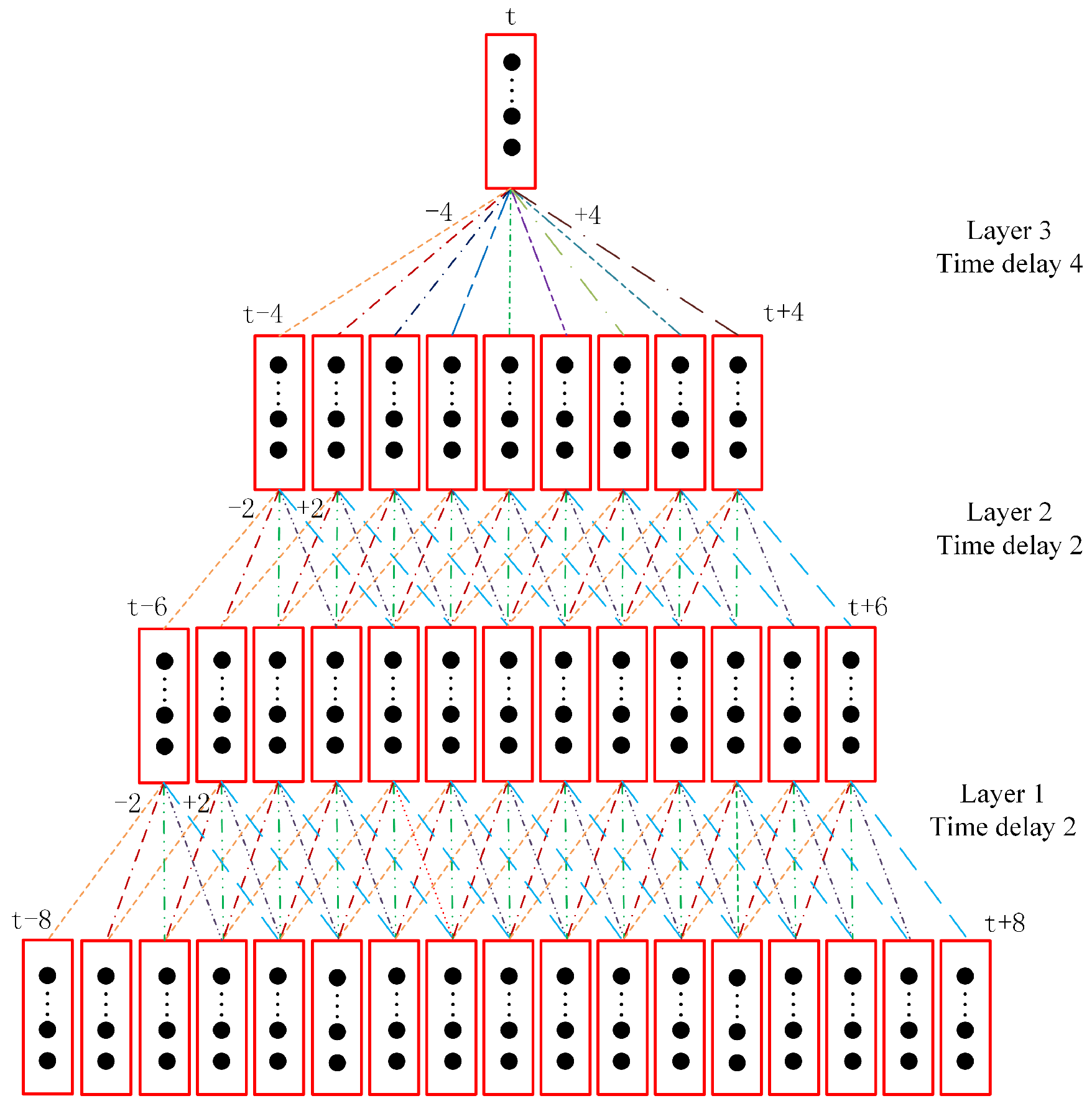
Based on the above, we explore the use of TDNN instead of RNN for slot filling. TDNN is a precursor of the convolutional network, also known as one-dimensional convolution. Especially, we used TDNN with symmetric delay offset, which can predict semantic labels by considering the same number of words before and after the target word. TDNN is a multi-layer neural network, with each layer having a strong ability for feature extraction, and also takes into account the long-term contexts. Unlike RNN, which inputs words in sentence order, TDNN is capable of simultaneously processing words that surround the target word. Moreover, TDNN is able to make use of arbitrary word contexts by setting different time delays rather than successive words with a context window. TDNN can get the contextual information of adjacent words surrounding the target word in sentence by context window and delay offsets.
To model even longer word contexts, it is straightforward to simply stack several TDNN layers to obtain a multi-layer TDNN due to its hierarchical multi-resolution nature. Particularly, the low layers of stacked TDNN deal with a narrow time context, which expands as information flows to higher layers [
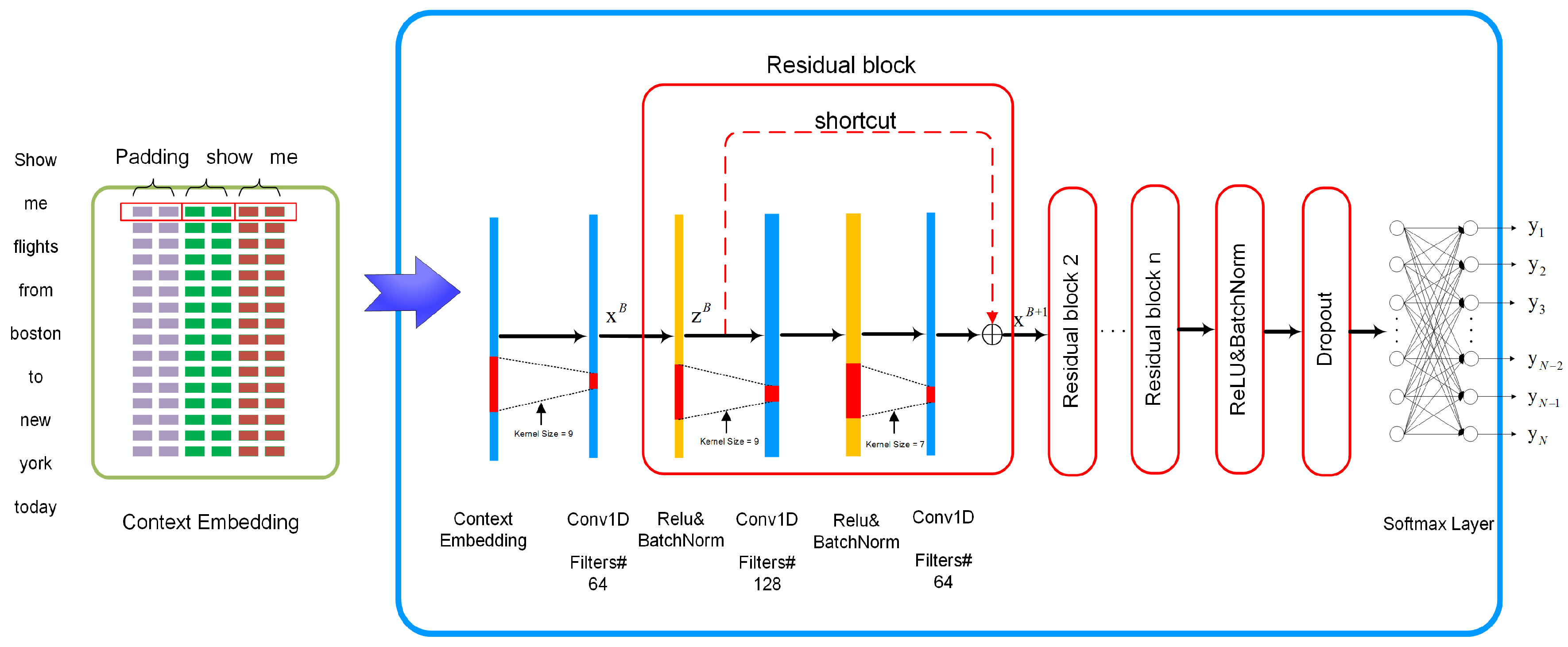
20]. Therefore, multi-layer TDNN can extract the context information of the target word from the sentence level instead of word level to predict the semantic label. However, with the deepening of the network, the gradient vanishing or exploding is an inevitable problem. Residual connection and gradient clip are two main methods to solve this problem. The residual CNN has shown to achieve good results on image classification tasks [21] and it has been proved that the residual structure can alleviate the gradient vanishing or exploding problems through skip connections. Therefore, we apply the residual structure to TDNN, which is named as ResTDNN. ResTDNN can fuse features which from different TDNN layers and strengthen feature propagation. Slot filling results show the superiority of ResTDNN to conventional RNN and its variants.
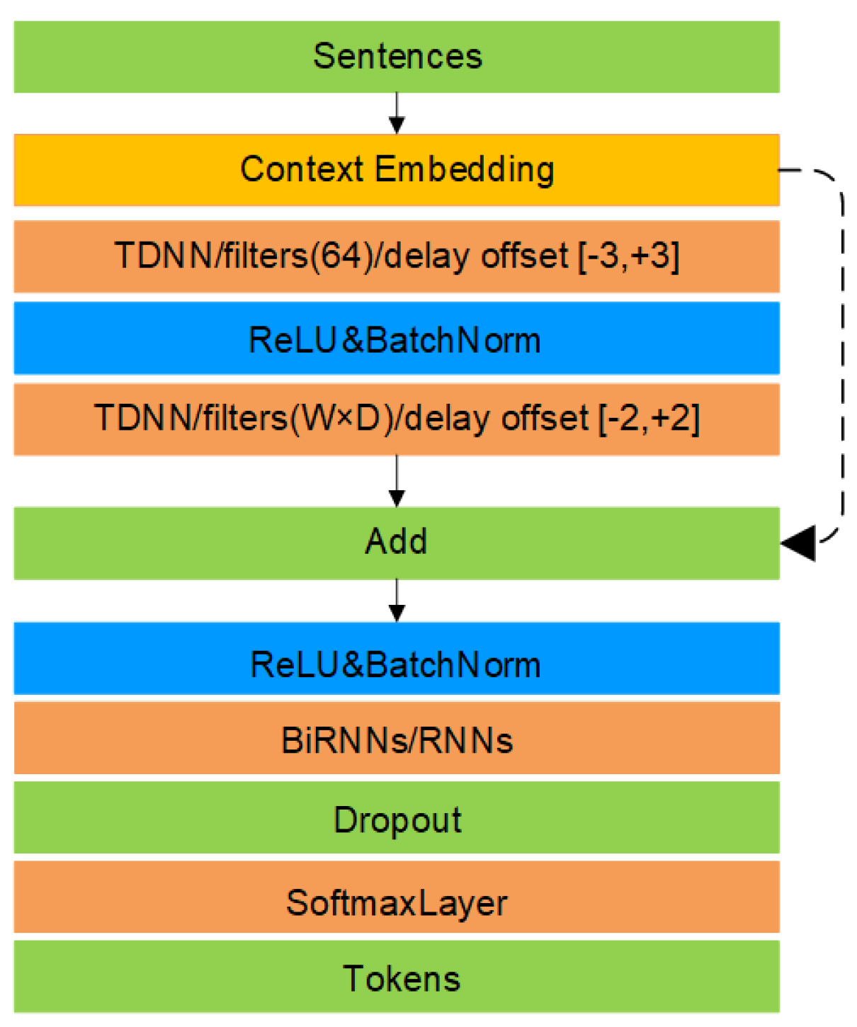
Inspired by the successful application of TDNN-BiLSTM to speech processing tasks, we combine a ResTDNN-based feature extractor with RNN (plain RNN, LSTM, GRU, and their bidirectional forms)-based classifier, to further improve the performance. Experimental results show that the combinations ResTDNN with back-end RNN achieve further improvement over the ResTDNN and RNN alone.
Recently, densely connected convolutional network (DenseNet) was proposed in [22], which connects each layer to every other layer in a feedforward fashion. DenseNet obtained significant improvements over the state-of-the-art on four highly competitive object recognition benchmark tasks, while requiring less computation to achieve high performance in image classification tasks. DenseNets have shown several remarkable advantages: alleviate the vanishing-gradient problem, strengthen feature propagation, encourage feature reuse, and enormously reduce the number of parameters.
Inspired by the DenseNets, we connect specific layers instead of every other layer in a feedforward fashion, which referred to as SC-TDNN later. Instead of using the skip connections that sums up the outputs of different TDNN layers in ResTDNN, the SC-TDNN reuses the feature from different TDNN layers, by which the representation of the target word conveys richer contextual information. Thus, the slot filling experiments yield comparable and even better performance through this method.
Similar to the aforementioned ResTDNN-RNN framework, we also experiment with the combination of SC-TDNN and RNN (and its variants as well). It is also seen that the combination of SC-TDNN with RNN achieves better results compared with those from SC-TDNN or RNN alone. In the final part of the paper, we compare the proposed models and methods with those from other literatures. We hope the experimental analysis and comparison provide useful insight for researchers in this area.
The remainder of the paper is organized as follows. Section 2 describes the related works, Section 3 shows the ResTDNN model, Section 4 presents the experimental results and analysis, and Section 5 draws the comparisons of previous results and summarizes our work.

2. Related Works

Neural network models, such as RNN and CNN, have been widely used in natural language processing (NLP) tasks. RNNs or their variants, such as LSTMs or GRUs, have been successfully applied in many different NLP tasks such as language modeling [23] or machine translation [24]. Deep learning has also been applied to intent detection and slot filling tasks of SLU [25,26]. Another important step forward is the invention of word embeddings [27,28], which transforms high-dimensional sparse vectors for word representations into low-dimensional dense vector representations in several natural language tasks [29,30]. RNN-EM [10] used RNN with external memory architecture and got a better slot filling result than pure RNN. Using CNNs is another trend for sequence labeling [29,30] or modeling larger units such as phrases [31] or sentences [32,33]. Distributed representations of words [27,28] are used as inputs for both models. Promising results were showed in the previous study [11], which combines CNN and CRF for sentence-level optimization.
RNN-LSTM architecture was proposed in [34] for joint modeling of slot filling, intent determination, and domain classification. They built a joint multi-domain model and investigated alternative architectures for modeling lexical context in spoken language understanding. The authors of [35] proposed a RNN based encoder–decoder model, which sums all of the encoded hidden states through an attention weight for predicting the utterance intent. A slot-gated mechanism [36] was proposed in order to focus on learning the relationship between intent and slot values. They obtained better semantic frame results by the global optimization. A capsule-based neural network model was proposed in [37] for accomplishing slot filling and intent detection. They proposed a dynamic routing-by-agreement schema for the SLU task. MPT-RNN [38] used triplets as an additional loss function based RNN model. They updated context window representation in order to make dissimilar samples more distant and similar samples close, and they got better classification results through this method. Although some pre-training models with external knowledge have worked well for many NLP tasks such as BERT-based model, large amounts of external data are often difficult to obtain and it also need large computing resources. In this paper, we study slot filling task under the single model framework and harness the time delay neural network to learn the feature representation of target word. Unlike pre-training model, our work is to conduct slot filling experiments without adding any external knowledge and additional resources. We only study the slot filling task in this work and conduct experiments with Air Travel Information System (ATIS) and SNIPS datasets.

3. The Proposed Model (ResTDNN)

3.1. Task Description

As mentioned, slot filling is a sequence labeling problem. Given a word sequence, the main purpose of slot filling is to predict slot tag for each word in the sentence. Table 1 gives a commonly used slot filling example in the ATIS [39] dataset. The sentence is a flight booking query Show me flights from Boston to New York today. The goal is to mark the word Boston as the beginning departure city (B-dept), New is marked as the beginning of the arrival city (B-arr) and York the ending of the arrival city (I-arr). today is tagged as the slot for the date (B-date). Other words in the sentence convey no meaning for the flight booking intention and are marked as slot O.

3.2. Time Delay Neural Networks

TDNN was first introduced in [15] for phoneme recognition. It is a multi-layer feedforward network. Figure 1 demonstrates the network structure of a basic TDNN. As shown, each output node of one layer depends on several adjacent nodes of its input. The input range is defined by a context delay offset [ d 1 , d 2 ] , where d 1 and d 2 represent the delay offsets. Dash lines of the same style [20] represent weight shared in each layer of TDNN, that is, the result of one-dimensional convolution is obtained by sliding the same convolution kernel. Specifically in the first input layer of Figure 1, when the delay offset is set to [ 2 , + 2 ] , the five consecutive frames are weighted by a layer-wise shared weight F as inputs to the activation function and the results are then normalized before fed into the next TDNN layer. For our task, each small rectangle of the input is a spliced m-dimensional word vectors corresponding to several successive words in the sentence. If the dimension of spliced word vectors is m, and the delay offset is [ d 1 , d 2 ] , the kernel size of the TDNN layer is ( d 2 d 1 + 1 ) × m . In the later experiments, we can also use multiple kernels to extract subspace information.

3.3. Residual Time Delay Neural Network

Here, we provide the model descriptions of the proposed ResTDNN. The model structural diagram of ResTDNN is described as follows and shown in Figure 2.

3.3.1. Embedding Layer

As in many NLP tasks, each of the input words is converted into a D-dimensional real-valued vector, namely, word embedding. We splice successive W word embeddings together where W is the splicing context size. Let w be the splicing context offset, the size of context window is W = 2 w + 1 . If there are not enough words before or after the target word for splicing, we fill there with padded word embeddings. Thus, the input at position t is
V t = [ v t w , v t 1 , v t , v t + 1 , v t + w ] .
For a sentence that contains N words, the vector representation of the entire sequence can be an input matrix s R N × ( W × D )
s = [ V 1 , V 2 , V 3 , , V N ] .

3.3.2. Time Delay Neural Network

Thus, for each target word, we form an embedding matrix M t R ( d 2 d 1 + 1 ) × ( W × D ) as the input to each TDNN hidden layer. In this paper, we use one-dimensional filter F (with width | F | = d 2 d 1 + 1 ) spanning all context embedding dimensions ( W × D ) . As described by the following equation
x t ( ) = M t ( ) F ( ) ,
where ∗ represents the convolution operation, x t ( ) is the convolutional result of the corresponding matrix M t from all words in the sentence. The number of filters is corresponding to the number of hidden layers in each TDNN’s layer.

3.3.3. ReLU and Batch Normalization

We use the Rectified Linear Unit (ReLU) [40] as the activation function to the output x t ( ) of the each TDNN layer. z t ( ) is the result of batch normalization [41] after the ReLU activation over the t-th input
z t ( ) = BatchNorm ( ReLU ( x t ( ) ) ) .

3.3.4. Residual Block

A residual operation can be represented as the follows,
x t ( B + 1 ) = F ( x t ( B ) ) + z t ( B ) ,
where x t ( B ) and x t ( B + 1 ) are the input and the output of the B-th residual block in the network, respectively, and F is the function of the residual network.

3.3.5. Dropout

To avoid overfitting when training the model, dropout [42] is adopted. The output of dropout layer for the t-th word is described as
g t = Dropout ( z t ( ) ) .

3.3.6. Softmax Layer

The softmax function is applied to the network to obtain the probability distribution y t of the t-th word:
y t = Softmax ( W s g t + b ) ,
where W s and b are, respectively, the weight and bias of the softmax layer.

3.4. ResTDNN-RNN Combination

ResTDNN can extract the contextual information of the target word, whereas the recurrent structure of RNN and its variants is able to capture the temporal change, which complements with ResTDNN. Thus, we superimpose ResTDNN onto RNN (including its variants) to check the improvement to the original model. As shown in Figure 3, we use ResTDNN followed by RNN (or its variants) to get a series of new model structures, which are named as ResTDNN-RNNs.

3.5. Objective Function

We use the softmax activation function as the last layer to obtain the normalized probability distribution, and the objective function used in this paper is based on cross-entropy [43],
L = 1 N t = 1 N c = 1 C y t , c log y ^ t , c ,
where y ^ t , c is the predicted probability of the c-th semantic tag of the t-th word and y t , c is the true probability of c-th semantic tag of t-th word in the sample. N is the number of words in the sample and C is the number of semantic tag categories.

4. Experiments

We carried out various experiments to demonstrate the performance of the TDNN. We hereby describe the experimental set-up, datasets, evaluation metrics, residual TDNN, skip concatenation TDNN, the combination of TDNN with RNNs (its variants), and the experimental results on ATIS and SNIPS datasets.

4.1. Experimental Setup

All the networks in the experiments were implemented using the TensorFlow deep learning toolkit. In model training, Stochastic Gradient Descent (SGD) was used in parameter optimization. The learning rate ( L r ) was initialized with a value of 0.5 unless otherwise specified and decreased to 0.9 times of the previous learning rate after every 10 epochs. We used a batch size of 1, L2 regularization [44] with λ = 1 e 5 and the dropout probability was set to p = 0.5 during model training. Unless otherwise stated, the dimension of the word embedding was set to E = 100 . Model specific parameters were presented in the table with the results. In order to avoid the gradient problem [45,46], gradient clipping with maximum L 2 -norm of 1 was applied when updated the parameters of model. To keep the length of the sentence constant after the delay operation, we set “padding=same” and “stride=1” when we used the one-dimensional convolution in the TensorFlow library. The weight parameters in the softmax layer and the word embeddings were initialized randomly with a uniform distribution in [ 0.2 , 0.2 ] .

4.2. Datasets

The proposed models and methods are evaluated on the widely used ATIS SLU dataset [47] and SNIPS NLU dataset [48]. The ATIS SLU dataset was collected from the air travel domain and consists of audio recordings of speakers making travel reservations. The training data consists of 3983 sentences with 56,590 words. The test data consists of 893 sentences with 9198 words. There are in total 127 semantic labels, including the label of the class O. There are a total of 25,509 slot occurrences in the training and test set. The SNIPS NLU dataset is a benchmark dataset to evaluate the performance of voice assistants. SNIPS NLU dataset includes 13,084 training sentences, 700 test sentences, and 700 validation sentences. There are 72 semantic labels and 112,421 words in SNIPS NLU dataset.

4.3. Evaluation Metrics

The slot filling results from the the proposed models are evaluated in terms of F1-score which has been widely used in many NLP tasks. F1-score is the harmonic average of P r e c i s i o n and R e c a l l . As described by the following equation,
F 1 = 2 × P r e c i s i o n × R e c a l l P r e c i s i o n + R e c a l l × 100 % ,
where
P r e c i s i o n = N W W N D × 100 % ,
R e c a l l = N W W N W × 100 % .
N W W is the number of tokens where the machine marks in consistence with the ground-truth. N D is the total number of slots labeled by the machine, and N W is the number of slots annotated by human in the transcriptions.

4.4. Results and Discussion

4.4.1. Results of RNN and its Variants

Here we present the slot filling results using traditional RNN and the commonly used variants (LSTM and GRU) and their bidirectional form (BiLSTM and BiGRU). To show the influence of context window size W, we first present the slot filling results from BiLSTM with different context window sizes. From Figure 4, we can see that the F1-score peaks at 95.32% when we increase the context window size W from 1 to 3, indicating that using longer word contexts benefits slot filling results. However, further increase W leads to degradation of F1. We may think that a shorter window size cannot fully utilize contextual semantic information, while a excessively long context window will potentially introduces additional noise to the model.
The slot filling results on two real-word datasets are presented in Table 2 along with the corresponding network configurations that achieves the best results. As shown in Table 2, RNN with LSTM or GRU cells achieves better F1-score than conventional RNN. It is observed that BiLSTM and BiGRU obtain better results than the unidirectional models, indicating the non-causal model which takes into account the future word information yields much better results. The BiGRU achieves the best F1-score (95.34%) among single RNN based models. Noted that in speech recognition, bidirectional models usually introduce unpleasant decoding latency, whereas in slot filling, the problem does not matter too much.

4.4.2. Results From Single Layer TDNN

Table 2, Table 3, Table 4 and Table 5 present the results obtained by single layer TDNN with different time delay steps D, splicing window size W and the number of filters K. Results show that long splicing window size is beneficial to semantic label prediction. As shown in Table 3, when 32 filters are used, the best performance can be obtained by using a splicing window size W = 5 and delay offset D = [ 4 , + 4 ] . When we increase the number of filters to 64, a better F1-score can be obtained by using W = 7 and D = [ 3 , + 3 ] . When we separately increase the splicing context size W and the delay offset D to a optimal, the performance of the one-layer TDNN model improves. As for the number of filters K, increasing the number of filters to 128 show similar results to those from using 64 filters. In the subsequent set of experiments, we only evaluate TDNN with K = 64 and K = 128 . It is also shown that results of TDNN with a single layer are comparable to those of RNN models, while the parameters of the former are much less.

4.4.3. Results From Multi-layer TDNN

Figure 5 presents slot filling results using multi-layer TDNN. The delay offset D, the number of filters K and the splicing window size W are set to values that have yielded the best results in the previous experiments. We increase the number of TDNN layers from 1 to 5 to check how the number of TDNN layers influence the results. As shown in Figure 5, network only one layer TDNN shows an F1-score of 94.84%. As we increase the number of layers from 1 to 5, the F1-score dropped monotonically to 93.82%. It can be seen to capture longer dependencies by simply increasing the number of TDNN layers fails to improve the performance. Model with deep network structure is difficult to train and may lead to gradient problem as well.

4.4.4. Results from ResTDNN

As shown from Figure 2, ResTDNN consists of sequentially stacked residual blocks. Each residual block contains two TDNN layers, two ReLU and normalization operations, and a shortcut that enforces the network to learn the residual content in each block. As aforementioned, by using residual structure, we can stack more TDNN layers and hence the performance of the models might be improved. We evaluate four network configurations, namely, ResTDNN-A to ResTDNN-D, with different numbers of TDNN layers and residual connections. The network configurations and the slot filling results are presented in Table 6. K d means the -th TDNN layer of the ResTDNN has a delay offset [ d , + d ] and the number of filters K. For example, 64 4 1 denotes the first TDNN layer of ResTDNN has 64 filters and the delay offset is [ 4 , + 4 ] . In Table 6, A ( 1 , 2 ) denotes the skip connection between the 1 -th and the 2 -th TDNN layer. For example, A ( 1 , 3 ) represents the summation of the outputs of the first TDNN layer and the third TDNN layer. The ResTDNN outperforms the multi-layer TDNN, indicating the effectiveness of the residual structure. The structure can strengthen feature propagation, alleviate the vanishing-gradient problem, and fuse the low-layer feature with the high-layer feature. The context information of feature which expands the wide as ResTDNN goes deep. As shown from experimental results, increasing the number of ResTDNN layers helps to improve the performance.
As shown in Table 6, the performance of ResTDNN-A with one residual block is 95.02% on ATIS dataset. When we increase the number of residual blocks, the performance of ResTDNN-B reaches 95.49% using two residual blocks and the best F1-score 95.51% is achieved using three residual blocks, which outperform the best one of RNNs. The F1-score of ResTDNN drops to 95.17% when we using the 9-layer TDNN. The performance of ResTDNN-B reachs 92.84% on the SNIPS NLU dataset.

4.4.5. Combining ResTDNN with RNN and Its Variants

In the previous sections we have conducted comparative experiments using RNN and its variants. Here, we conduct experiments to show the effect of the performance of ResTDNN followed by RNN and its variants (LSTM, GRU, and bidirectional forms). The network configurations and corresponding results are presented in Table 7. The ResTDNN used here contains multi-layer TDNN with residual structure, which fuses features from different TDNN layers.
By comparing the results presented in Table 2 and Table 7, we can see that the combination of ResTDNN with RNNs (LSTM, GRU, and bidirectional variants) effectively improves the slot filling performance than those of original RNN and its variants. It is seen ResTDNN-BiLSTM achieved an result of 95.62% in terms of F1-score on ATIS dataset, an improvement of 0.3% compared with BiLSTM only. As can be seen from Table 2 and Table 7, the performance of RNN and its variants also get significantly improvements on SNIPS dataset after combining with ResTDNN. These results indicate that the ResTDNN, as a feature extraction model, gets better representation of the input words. By comparing the result of ResTDNN-BiLSTM (95.62%) with that of ResTDNN (95.51%), the BiLSTM shows better capability of capturing the temporal change of the inputs.

4.4.6. Stacked TDNN with Skip Concatenation

Figure 6 shows the diagram block of the SC-TDNN. As shown, SC-TDNN consists of sequentially skip concatenation of the outputs of different TDNN blocks. The structure of SC-TDNN is similar to ResTDNN and they have the same number of layers, despite that the features from different layers are spliced instead of being summed together in ResTDNN. The number of filters and kernel size in each layer of SC-TDNN are also identical to those in the corresponding layers of ResTDNN. Table 8 presents the network structure and the results. Four network configurations denoted as SC-TDNN-A to SC-TDNN-D are evaluated, each with different number of layers and skip concatenation operation. It is shown that SC-TDNN outperforms the multi-layer TDNN and also obtains a better F1 result than pure ResTDNN, indicating the effectiveness of feature reuse.
As shown in Table 8, the performance of SC-TDNN-A with one skipped concatenation is 95.10%. By increasing the number of layers and the number of skip concatenations, SC-TDNN-C reaches best F1-score of 95.73% on ATIS dataset. SC-TDNN-C obtains 92.94% F1-score on SNIPS NLU dataset. It is also observed that SC-TDNN gets better result over ResTDNN only. When we further adding TDNN blocks from SC-TDNN-C, the performance of the model decreases afterwards.

4.4.7. Combining SC-TDNN with RNNs

Similar to ResTDNN-RNN, we also experiment with the combination of SC-TDNN with RNN (including its variants), namely, SC-TDNN-RNN. The structure of SC-TDNN-RNN is shown in Figure 7. We use SC-TDNN as the feature extractor for RNN-based sequence classifier. The network configurations and results are presented in Table 9. The SC-TDNN used here is multi-layer TDNN with skip concatenation, which reuse feature from different TDNN layer.
By comparing the results in Table 9 of SC-TDNN and the results in Table 2 obtained by single RNN (or its variants), the slot filling performance has been effectively improved by combining the SC-TDNN front-end with RNN (or its variants) back-end. It is also observed that SC-TDNN-BiGRU achieves a result of 95.66% in terms of F1-score, an absolute improvement of 0.32% compared with BiGRU only. SC-TDNN-BiLSTM obtains a 92.91% F1-score on the SNIPS NLU dataset, and gets a 1.2% improvement than the performance of model which use BiLSTM only. It shows that the difference of performance between the unidirectional and bidirectional structures of the model become marginal after the combination, i.e., the unidirectional RNN and its variants get similar results with the bidirectional ones when combined with SC-TDNN. These indicate that SC-TDNN, as a feature extraction model, is underlying a uncausal model for learning representations of the input word sequence.

5. Comparisons and Conclusions

5.1. Comparisons of Previous Results

Finaly, in Table 10, we present several previous slot filling results on ATIS and SNIPS datasets reported in literature including our best results.The previous best result was achieved by using mining polysemous triplets with Recurrent Neural Networks (MPT-RNN). According to Table 10, our SC-TDNN-C outperforms the previous best models without any additional features or data sources. Finally, we combined our proposed models with RNNs to observe the performance gains of models to the RNNs. The experimental results show that the combination futher improves the performance of RNNs. Experiment results on ATIS and SNIPS datasets for slot filling task show that the semantic label of target word is largely depended on its adjacent words. Using ResTDNN and SC-TDNN can fuse the feature representation of target word and its adjacent words, thus proposed models get better performance than the RNN model, which directly inputs the representation of target word.

5.2. Conclusions

We have investigated the use of TDNN in the slot filling task in spoken language understanding, with particular attention to modeling the contexts of input words. Based on the fact that directly stacking several TDNN layers does not lead to better results, we proposed the residual TDNN (ResTDNN) and skip concatenation TDNN (SC-TDNN), which are inspired by the ResCNNs and DenseNet respectively. The ResTDNN used skip connections between different layers and the SC-TDNN concatenated the outputs of different layers. The proposed network structures can either fuse the features from different TDNN layers or allow feature reuse through the networks, and hence consequently learned more complex contextual information. Slot filling experimental results showed the effectiveness of the proposed method. We further improved the network by combining the TDNN networks with followed RNNs and observed consistent performance gain over single RNN.

Author Contributions

Conceptualization, Z.Z. and H.H.; Methodology, Z.Z.; Software, Z.Z.; Validation, K.W. and H.H.; Formal analysis, Z.Z.; Writing—original draft preparation, Z.Z.; Writing—review and editing, Z.Z. All authors read and agreed to the published version of the manuscript.

Funding

This work was supported by the National Key R&D Program of China ( 2017YFB1402101), Natural Science Foundation of China (61663044, 61761041), the Key Science and Technology Project of Xinjiang (No.2016A03007-1), and the Higher Education Innovation Project of Xinjiang (XJEDU2017T002).

Conflicts of Interest

The authors declare no conflicts of interest.

References

  1. Zhang, X.; Wang, H. A joint model of intent determination and slot filling for spoken language understanding. IJCAI 2016, 16, 2993–2999. [Google Scholar]
  2. Tur, G.; Deng, L. Intent determination and spoken utterance classification. In Spoken Language Understanding: Systems for Extracting Semantic Information from Speech; Wiley: Chichester, UK, 2011; pp. 93–118. [Google Scholar]
  3. Yaman, S.; Deng, L.; Yu, D.; Wang, Y.-Y.; Acero, A. An integrative and discriminative technique for spoken utterance classification. IEEE Trans. Audio Speech Lang. Process. 2008, 16, 1207–1214. [Google Scholar] [CrossRef]
  4. Mikolov, T.; Karafiát, M.; Burget, L.; Černockỳ, J.; Khudanpur, S. Recurrent neural network based language model. In Proceedings of the Eleventh Annual Conference of the International Speech Communication Association, Chiba, Japan, 26–30 September 2010. [Google Scholar]
  5. Yao, K.; Zweig, G.; Hwang, M.-Y.; Shi, Y.; Yu, D. Recurrent neural networks for language understanding. Interspeech 2013, 2524–2528. [Google Scholar]
  6. Raymond, C.; Riccardi, G. Generative and discriminative algorithms for spoken language understanding. In Proceedings of the Eighth Annual Conference of the International Speech Communication Association, Antwerp, Belgium, 27–31 August 2007. [Google Scholar]
  7. Wang, Y.-Y.; Acero, A. Discriminative models for spoken language understanding. In Proceedings of the Ninth International Conference on Spoken Language Processing, Jeju, Korea, 17–21 September 2006. [Google Scholar]
  8. Dahl, G.E.; Yu, D.; Deng, L.; Acero, A. Context-dependent pre-trained deep neural networks for large-vocabulary speech recognition. IEEE Trans. Audio Speech Lang. Process. 2011, 20, 30–42. [Google Scholar] [CrossRef] [Green Version]
  9. Jelinek, F.; Lafferty, J.D.; Mercer, R.L. Basic methods of probabilistic context free grammars. In Speech Recognition and Understanding; Springer: London, UK, 1992; pp. 345–360. [Google Scholar]
  10. Peng, B.; Yao, K. Recurrent neural networks with external memory for language understanding. arXiv 2015, arXiv:1506.00195. [Google Scholar]
  11. Xu, P.; Sarikaya, R. Convolutional neural network based triangular crf for joint intent detection and slot filling. In Proceedings of the 2013 IEEE Workshop on Automatic Speech Recognition and Understanding, Olomouc, Czech Republic, 8–13 December 2013; pp. 78–83. [Google Scholar]
  12. Mesnil, G.; Dauphin, Y.; Yao, K.; Bengio, Y.; Deng, L.; Hakkani-Tur, D.; He, X.; Heck, L.; Tur, G.; Yu, D.; et al. Using recurrent neural networks for slot filling in spoken language understanding. IEEE/ACM Trans. Audio Speech Lang. Process. 2014, 23, 530–539. [Google Scholar] [CrossRef]
  13. Yao, K.; Peng, B.; Zhang, Y.; Yu, D.; Zweig, G.; Shi, Y. Spoken language understanding using long short-term memory neural networks. In Proceedings of the 2014 IEEE Spoken Language Technology Workshop (SLT), South Lake Tahoe, NV, USA, 7–10 December 2014; pp. 189–194. [Google Scholar]
  14. Waibel, A. Modular construction of time-delay neural networks for speech recognition. Neural Comput. 1989, 1, 39–46. [Google Scholar] [CrossRef]
  15. Waibel, A.; Hanazawa, T.; Hinton, G.; Shikano, K.; Lang, K.J. Phoneme recognition using time-delay neural networks. IEEE Trans. Acoustics Speech Signal Process. 1989, 37, 328–339. [Google Scholar] [CrossRef]
  16. Snyder, D.; Garcia-Romero, D.; Sell, G.; Povey, D.; Khudanpur, S. X-vectors: Robust dnn embeddings for speaker recognition. In Proceedings of the 2018 IEEE International Conference on Acoustics, Speech and Signal Processing (ICASSP), Calgary, AB, Canada, 15–20 April 2018; pp. 5329–5333. [Google Scholar]
  17. Kershaw, D.J.; Robinson, A.J.; Hochberg, M. Context-dependent classes in a hybrid recurrent network-hmm speech recognition system. In Advances in Neural Information Processing Systems; Springer: London, UK, 1996; pp. 750–756. [Google Scholar]
  18. Povey, D.; Ghoshal, A.; Boulianne, G.; Burget, L.; Glembek, O.; Goel, N.; Hannemann, M.; Motlicek, P.; Qian, Y.; Schwarz, P. The Kaldi Speech Recognition Toolkit; Idiap: Martigny, Switzerland, 2012. [Google Scholar]
  19. Hochreiter, S.; Bengio, Y.; Frasconi, P.; Schmidhuber, J. Gradient Flow in Recurrent Nets: The Difficulty of Learning Long-term Dependencies; Wiley Press: Hoboken, NJ, USA, 2001. [Google Scholar]
  20. Peddinti, V.; Povey, D.; Khudanpur, S. A time delay neural network architecture for efficient modeling of long temporal contexts. In Proceedings of the Sixteenth Annual Conference of the International Speech Communication Association, Dresden, Germany, 6–10 September 2015. [Google Scholar]
  21. Zhong, Z.; Li, J.; Ma, L.; Jiang, H.; Zhao, H. Deep residual networks for hyperspectral image classification. In Proceedings of the 2017 IEEE International Geoscience and Remote Sensing Symposium (IGARSS), Fort Worth, TX, USA, 23–28 July 2017; pp. 1824–1827. [Google Scholar]
  22. Huang, G.; Liu, Z.; Maaten, L.v.; Weinberger, K.Q. Densely connected convolutional networks. In Proceedings of the IEEE Conference on Computer Vision and Pattern Recognition, Honolulu, HI, USA, 21–26 July 2017. [Google Scholar]
  23. Mikolov, T.; Kombrink, S.; Burget, L.; Černockỳ, J.; Khudanpur, S. Extensions of recurrent neural network language model. In Proceedings of the 2011 IEEE International Conference on Acoustics, Speech and Signal Processing (ICASSP), Prague, Czech Republic, 22–27 May 2011; pp. 5528–5531. [Google Scholar]
  24. Brown, P.F.; Cocke, J.; Pietra, S.A.D.; Pietra, V.J.D.; Jelinek, F.; Lafferty, J.D.; Mercer, R.L.; Roossin, P.S. A statistical approach to machine translation. Comput. Linguist. 1990, 16, 79–85. [Google Scholar]
  25. Deng, L.; Tur, G.; He, X.; Hakkani-Tur, D. Use of kernel deep convex networks and end-to-end learning for spoken language understanding. In Proceedings of the 2012 IEEE Spoken Language Technology Workshop (SLT), Miami, FL, USA, 2–5 December 2012; pp. 210–215. [Google Scholar]
  26. Tur, G.; Deng, L.; Hakkani-Tür, D.; He, X. Towards deeper understanding: Deep convex networks for semantic utterance classification. In Proceedings of the 2012 IEEE International Conference on Acoustics, Speech and Signal Processing (ICASSP), Kyoto, Japan, 25–30 March 2012; pp. 5045–5048. [Google Scholar]
  27. Bengio, Y.; Ducharme, R.; Vincent, P.; Jauvin, C. A neural probabilistic language model. J. Mach. Learn. Res. 2003, 3, 1137–1155. [Google Scholar]
  28. Mikolov, T.; Chen, K.; Corrado, G.; Dean, J. Efficient estimation of word representations in vector space. arXiv 2013, arXiv:1301.3781. [Google Scholar]
  29. Collobert, R.; Weston, J. A unified architecture for natural language processing: Deep neural networks with multitask learning. In Proceedings of the 25th International Conference on Machine Learning; ACM: New York, NY, USA, 2008; pp. 160–167. [Google Scholar]
  30. Collobert, R.; Weston, J.; Bottou, L.; Karlen, M.; Kavukcuoglu, K.; Kuksa, P. Natural language processing (almost) from scratch. J. Machine Learn. Res. 2011, 12, 2493–2537. [Google Scholar]
  31. Yin, W.; Schütze, H. Multigrancnn: An architecture for general matching of text chunks on multiple levels of granularity. In Proceedings of the 53rd Annual Meeting of the Association for Computational Linguistics and the 7th International Joint Conference on Natural Language Processing (Volume 1: Long Papers), Beijing, China, 26–31 July 2015; pp. 63–73. [Google Scholar]
  32. Kalchbrenner, N.; Grefenstette, E.; Blunsom, P. A convolutional neural network for modelling sentences. arXiv 2014, arXiv:1404.2188. [Google Scholar]
  33. Kim, Y. Convolutional neural networks for sentence classification. arXiv 2014, arXiv:1408.5882. [Google Scholar]
  34. Hakkani-Tür, D.; Tur, G.; Celikyilmaz, A.; Chen, Y.N.; Wang, Y.Y. Multi-domain joint semantic frame parsing using bidirectional rnn-lstm. In Proceedings of the 17th Annual Meeting of the International Speech Communication Association (INTERSPEECH 2016), San Francisco, CA, USA, 8–12 September 2016. [Google Scholar]
  35. Liu, B.; Lane, I. Attention-based recurrent neural network models for joint intent detection and slot filling. Interspeech 2016, 2016, 685–689. [Google Scholar]
  36. Goo, C.-W.; Gao, G.; Hsu, Y.-K.; Huo, C.-L.; Chen, T.-C.; Hsu, K.-W.; Chen, Y.-N. Slot-gated modeling for joint slot filling and intent prediction. In Proceedings of the 2018 Conference of the North American Chapter of the Association for Computational Linguistics: Human Language Technologies, Volume 2 (Short Papers), New Orleans, LA, USA, 1–6 June 2018; pp. 753–757. [Google Scholar]
  37. Zhang, C.; Li, Y.; Du, N.; Fan, W.; Yu, P.S. Joint slot filling and intent detection via capsule neural networks. arXiv 2018, arXiv:1812.09471. [Google Scholar]
  38. Vukoti, V.; Raymond, C. Mining polysemous triplets with recurrent neural networks for spoken language understanding. Interspeech 2019, 2019. [Google Scholar]
  39. Price, P.J. Evaluation of spoken language systems: The atis domain. In Proceedings of the third DARPA Speech and Natural Language Workshop, Hidden Valley, PA, USA, 24–27 June 1990. [Google Scholar]
  40. Dahl, G.E.; Sainath, T.N.; Hinton, G.E. Improving deep neural networks for lvcsr using rectified linear units and dropout. In Proceedings of the 2013 IEEE International Conference on Acoustics, Speech and Signal Processing, Vancouver, BC, Canada, 26–31 May 2013; pp. 8609–8613. [Google Scholar]
  41. Ioffe, S.; Szegedy, C. Batch normalization: Accelerating deep network training by reducing internal covariate shift. arXiv 2015, arXiv:1502.03167. [Google Scholar]
  42. Hinton, G.E.; Srivastava, N.; Krizhevsky, A.; Sutskever, I.; Salakhutdinov, R.R. Improving neural networks by preventing co-adaptation of feature detectors. arXiv 2012, arXiv:1207.0580. [Google Scholar]
  43. Veselỳ, K.; Ghoshal, A.; Burget, L.; Povey, D. Sequence-discriminative training of deep neural networks. Interspeech 2013, 2013, 2345–2349. [Google Scholar]
  44. Phillips, D.L. A technique for the numerical solution of certain integral equations of the first kind. J. ACM (JACM) 1962, 9, 84–97. [Google Scholar] [CrossRef]
  45. Bengio, Y.; Simard, P.; Frasconi, P. Learning long-term dependencies with gradient descent is difficult. IEEE Trans. Neural Netw. 1994, 5, 157–166. [Google Scholar] [CrossRef] [PubMed]
  46. Glorot, X.; Bengio, Y. Understanding the difficulty of training deep feedforward neural networks. In Proceedings of the Thirteenth International Conference on Artificial Intelligence and Statistics, Sardinia, Italy, 13–15 May 2010; pp. 249–256. [Google Scholar]
  47. Hemphill, C.T.; Godfrey, J.J.; Doddington, G.R. The atis spoken language systems pilot corpus. In Proceedings of the Speech and Natural Language: Proceedings of a Workshop, Hidden Valley, PA, USA, 24–27 June 1990. [Google Scholar]
  48. Coucke, A.; Saade, A.; Ball, A.; Bluche, T.; Caulier, A.; Leroy, D.; Doumouro, C.; Gisselbrecht, T.; Caltagirone, F.; Lavril, T. Snips voice platform: An embedded spoken language understanding system for private-by-design voice interfaces. arXiv 2018, arXiv:1805.10190. [Google Scholar]
Figure 1. Structure of Time Delay Neural Network (TDNN).
Symmetry 12 00993 g001
Figure 2. Structure of Residual Time Delay Neural Network (ResTDNN).
Symmetry 12 00993 g002
Figure 3. Structure of ResTDNN-RNNs.
Symmetry 12 00993 g003
Figure 4. Results on ATIS dataset of different context window sizes in BiLSTM SLU model.
Symmetry 12 00993 g004
Figure 5. Slot filling results on ATIS dataset using multi-layer TDNN.
Symmetry 12 00993 g005
Figure 6. Structure of SC-TDNN-C.
Symmetry 12 00993 g006
Figure 7. Structure of SC-TDNN-RNNs.
Symmetry 12 00993 g007
Table 1. Examples of ATIS sentence and the annotated slots.
SentenceShowmeflightsfromBostontoNewYorktoday
SlotsOOOOB-deptOB-arrI-arrB-date
SentenceTellmeaboutgroundtransportationinSt.Petersburgairport
SlotsOOOOOOB-airport_nameI-airport_nameI-airport_name
Table 2. Slot filling results on two real-word datasets using RNN and its variants.
Model [ W , E , H , Lr ] SNIPS (F1)ATIS (F1)
RNN [ 3 , 100 , 50 , 0.1 ] 87.4294.50
LSTM [ 3 , 100 , 100 , 0.5 ] 89.7994.87
GRU [ 3 , 100 , 100 , 0.5 ] 90.2395.03
BiRNN [ 7 , 100 , 100 , 0.5 ] 89.3694.94
BiLSTM [ 3 , 100 , 100 , 0.5 ] 91.7195.32
BiGRU [ 3 , 50 , 100 , 0.6 ] 91.8095.34
W = Splicing windows size; E = Word embedding vector dimension; H = Hidden layer size; L r = Initial learning rate.
Table 3. Slot filling results on ATIS dataset using single-layer TDNN with 32 filters.
Delay OffsetsW = 3579
PRF1PRF1PRF1PRF1
[ 1 , + 1 ] 91.1992.3291.7592.5093.0992.8093.2993.6293.4693.9494.5794.26
[ 2 , + 2 ] 92.3293.2392.7793.3493.8793.6093.9694.4094.1893.7994.7194.25
[ 3 , + 3 ] 93.4294.0893.7593.9394.4094.1694.2894.7894.5394.3894.6494.51
[ 4 , + 4 ] 93.6794.4394.0594.2395.0394.6394.1894.7194.4594.1894.6494.41
Table 4. Slot filling results on ATIS dataset using single-layer TDNN with 64 filters.
Delay OffsetsW = 3579
PRF1PRF1PRF1PRF1
[ 1 , + 1 ] 91.4292.4591.8892.6893.3493.0193.2893.9793.6393.9894.6894.33
[ 2 , + 2 ] 92.3993.3492.8693.7194.0893.9094.0994.3694.2394.0594.7594.40
[ 3 , + 3 ] 93.5194.0193.7693.9494.6194.2794.6994.9994.8494.3495.1094.72
[ 4 , + 4 ] 94.2894.7194.5094.6294.7894.7094.6095.0394.8194.4994.8994.69
Table 5. Slot filling results on ATIS dataset using single-layer TDNN with 128 filters.
Delay OffsetsW = 3579
PRF1PRF1PRF1PRF1
[ 1 , + 1 ] 91.1892.6091.8992.7193.6993.2093.3594.0493.7094.5494.6494.59
[ 2 , + 2 ] 92.3993.2392.8193.5793.9493.7694.4694.3694.4194.7694.8994.82
[ 3 , + 3 ] 93.3993.5893.4994.2094.5494.3794.8294.8594.8494.4594.8294.64
[ 4 , + 4 ] 94.5094.4394.4694.2594.7594.5094.7894.6894.7394.5894.7194.65
Table 6. Results on two real-word datasets using residual TDNN.
Models { [ K d ] , A ( 1 , 2 ) } SNIPS (F1)ATIS (F1)
ResTDNN-A { [ 64 4 1 , 128 4 2 , 64 3 3 ] , A ( 1 , 3 ) } 91.4095.02
ResTDNN-B + { [ 128 2 4 , 64 4 5 ] , A ( 3 , 5 ) } 92.8495.49
ResTDNN-C + { [ 128 3 6 , 64 4 7 ] , A ( 5 , 7 ) } 92.2395.51
ResTDNN-D + { [ 128 3 8 , 64 4 9 ] , A ( 7 , 9 ) } 92.1495.17
ResTDNN-B to ResTDNN-D are derived from ResTDNN-A by incrementally adding an additional residual block. The additional block configurations are denoted as a ’+’ for ResTDNN-B to ResTDNN-D.
Table 7. Results on combination ResTDNN with RNN and its variants of two real-word datasets.
Models [ W , E , H , Lr ] SNIPS (F1)ATIS (F1)
ResTDNN-RNN [ 3 , 50 , 100 , 0.5 ] 90.4995.11
ResTDNN-LSTM [ 3 , 100 , 100 , 0.5 ] 91.7195.18
ResTDNN-GRU [ 3 , 50 , 100 , 0.5 ] 91.4795.23
ResTDNN-BiRNN [ 3 , 100 , 100 , 0.45 ] 91.2795.37
ResTDNN-BiLSTM [ 3 , 100 , 100 , 0.5 ] 92.1595.62
ResTDNN-BiGRU [ 3 , 50 , 100 , 0.65 ] 92.1795.55
Table 8. Results on two real-word datasets using SC-TDNN.
Models { [ K d ] , S ( 1 , 2 ) } SNIPS (F1)ATIS (F1)
SC-TDNN-A { [ 64 4 1 , 128 4 2 ] , S ( 1 , 2 ) } 91.3595.10
SC-TDNN-B { [ 64 4 1 , 128 4 2 , 64 3 3 ] , S ( 1 , 3 ) } 92.2795.52
SC-TDNN-C + { [ 128 2 4 , 64 4 5 ] , S ( 3 , 5 ) } 92.9495.73
SC-TDNN-D + { [ 128 3 6 , 64 4 7 ] , S ( 5 , 7 ) } 92.4795.27
S represents operation that splicing together the activated normalization output of 1 -th TDNN layer and output of 2 -th TDNN layer. SC-TDNN-C and SC-TDNN-D are derived from SC-TDNN-B by incrementally adding an skip concatenation block. The block configurations are denoted as a ’+’ for SC-TDNN-C to SC-TDNN-D. S ( 1 , 2 ) denotes the skip concatenation between the 1 -th and the 2 -th TDNN layer.
Table 9. ATIS and SNIPS results on combination of SC-TDNN and RNNs.
Model [ W , E , H , Lr ] SNIPS (F1)ATIS (F1)
SC-TDNN-RNN [ 3 , 100 , 100 , 0.5 ] 92.0795.37
SC-TDNN-LSTM [ 3 , 100 , 100 , 0.5 ] 92.8195.60
SC-TDNN-GRU [ 3 , 100 , 100 , 0.5 ] 92.5095.54
SC-TDNN-BiRNN [ 3 , 100 , 100 , 0.5 ] 92.0695.38
SC-TDNN-BiLSTM [ 3 , 100 , 100 , 0.5 ] 92.9195.59
SC-TDNN-BiGRU [ 3 , 100 , 100 , 0.5 ] 92.8095.66
Table 10. ATIS benchmark results reported in literature.
MethodsSNIPS (F1)ATIS (F1)
CNN [11]-94.35
LSTM [13]-94.85
Attention BiRNN [35]87.8094.20
Joint Seq. [34]87.3094.20
Slot-Gated Full Atten. [36]88.8094.80
RNN-EM [10]-95.25
CAPSULE-NLU [37]91.8095.20
MPT-RNN [38]88.0195.66
ResTDNN-B92.8495.49
ResTDNN-BiLSTM92.1595.62
SC-TDNN-C92.9495.73
SC-TDNN-BiGRU92.8095.66

