Unified Fundamental Formulas for Static Analysis of Pin-Jointed Bar Assemblies

Abstract

The initial axial forces of members—whatever caused by prestress or external loads—may strongly change the mechanical properties of pin-jointed bar assemblies, to enhance, or even establish their structural stiffness. The structural responses under external disturbance cannot be calculated accurately if the influence of initial axial forces has not been considered appropriately. In this paper, an analytic theory considering the effect of initial internal forces is developed on the basis of linear elasticity hypothesis. The fundamental formulas proposed finally include generalized equilibrium equations and generalized compatibility equations, both of which have square coefficient matrices of full rank being transposed with each other. Generally, this method can be regarded as an extended version of a traditional force method considering the stiffening effect of initial internal forces. Compared with the matrix force method, it has a wider application scenario since few redundant simplifications are employed in the derivation of the formulas. In comparison with the displacement-based algorithm, the proposed method has the inherent advantages of the force method—the physical concepts of each item in equations are fairly explicit; and the combination coefficients of self-stress states and mechanisms are determined simultaneously in solving the structural responses. Thus, it is very helpful for us to essentially comprehend the principle that the pin-jointed bar assemblies resist the external loads.

1. Introduction

Pin-jointed bar assemblies are becoming increasingly popular in structural engineering. The concepts of statical and kinematical determinacy are key to understanding the mechanics of these kinds of structures. A pin-jointed framework is clearly statically determinate if the internal force in each bar can be determined by means of the equations of equilibrium for a given set of external loads applied at the nodes.

Then, the addition of any extra bars will make the framework become statically indeterminate. There are more unknowns than equations of equilibrium, and the solution for the bar tensions is not unique [1]. On the other hand, a pin-jointed framework is said to be kinematically determinate in the sense that the position of the nodes can be uniquely determined by the lengths of the bars. However, if any bars of the frame are removed, the resulting assembly becomes kinematically determinate, since the location of the nodes is not now uniquely determined by the length of the bars [2,3].

Thus far, the most commonly used classification criterion for them is proposed by Pellegrino and Calladine [4], depending on whether the assembly is statically determinate or indeterminate, and whether kinematically determinate or indeterminate (see Table 1).

Table 1. Four different types of structural assemblies.

Assembly Type	Statical and Kinematical Properties
I	Statically determinate and kinematically determinate
II	Statically indeterminate and kinematically determinate
III	Statically determinate and kinematically indeterminate
IV	Statically indeterminate and kinematically indeterminate

The prestressed bar systems are limited to type II and type IV assemblies since they need, at least, one state of self-stress in the absence of external loads, i.e., to be statically indeterminate [5]. The cable-strut systems are the typical examples of type II or type IV, including cable trusses, cable domes, tensegrity structures, etc. The introduction of prestress for type II assemblies can improve their structural stiffness and limit the components to linear-elastic states under loads, while the assemblies of type IV rely on prestress to achieve stiffness, and also to prevent any cable segments or fabric panels from becoming slack [6,7]. Even a type III assembly possessing no self-stress states (say a hanging cable or a cable net) can also become stable when the vector of nodal loads is orthogonal to its mechanisms [8,9], which is very similar to the principle that prestress stiffens the mechanisms of type IV assemblies.

The common feature of the foregoing cases is that the initial internal forces, no matter if caused by prestress or external loads, significantly changes the static characteristics of the structures. Particularly, it affects the stiffness of the structures, which should be taken into account in the calculation of the structural response under external loads [10]. At present, there are two kinds of methods to consider the initial internal forces in static analysis. One of them can be classified as the displacement-based method, such as the Finite Element Method, in which the so-called geometrical stiffness matrix is incorporated into the tangent stiffness matrix [11,12,13]. Then, the analysis of type III and IV assemblies poses no difficulty, because the modified tangent stiffness matrices have full rank. The other kind is the matrix force method, proposed and developed by many scholars [14,15,16,17], where the analysis of the equilibrium matrix is performed to determine the kinematic determinacy and states of the self-stress. By introducing the so-called product-force vectors, the traditional equilibrium matrix is modified to meet the condition of full row rank.

As we know, displacement-based methods can be conveniently programmed to consider the geometric nonlinearities numerically. To resort to iterative schemes for the above structures, as described by Kaveh [18], the deformations due to any load condition, or the structural response to a design change, can be calculated with high accuracy. However, this kind of approach does not provide much insight, and no rough estimates can be made. In contrast, because the matrix force methods are based on the singular value decomposition on the asymmetric equilibrium matrices, the computation requires a large amount of computer memory and, thus, becomes computationally expensive [15]. Even so, the force method has its inherent advantages: the physical concepts of each item in equations are fairly explicit; the essential structural and kinematic properties, e.g., the rigid body motions or infinitesimal mechanisms, the states of self-stress, etc., can be explained clearly from the orthogonal subspace of the equilibrium matrix. It has made the matrix force method complementary to the displacement-based method and irreplaceable in the design of pin-jointed bar assemblies. Paradoxically, the basic equations used in the present matrix force method have some limitations—to keep the conciseness in form, excessive hypotheses have been made in the derivation of the formulas, which may narrow their application scope; various but fragmented equations have been produced for specialized applications, which may lead to a puzzle of choice. Hence, it is necessary to seek a set of unified fundamental formulas, being fit for a general linear static analysis of pin-jointed bar assemblies. Meanwhile, the proposed formulas should keep an acceptable complexity in form, and reduce to the fundamental formulas of traditional force method when they are applied to type I assemblies without initial internal forces. This paper deals with this matter, aims to extend the important work given by Pellegrino and Calladine [4,14] and broaden its application scenarios further.

The layout of the paper is as follows. In Section 2, starting from the incremental form of equilibrium equations, as well as the compatibility equations, an analytic theory considering the effect of initial internal forces is developed on the basis of linear elasticity hypothesis. Then, the axial force variables and displacement variables are decoupled by means of linear algebra and the Moore–Penrose generalized inverse theory in Section 3. The fundamental formulas, including generalized equilibrium equations and generalized compatibility equations are obtained, without sacrificing the insight that the traditional force methods give. Section 4 investigates the correlations between this method and earlier work commonly used. It is followed by several examples in Section 5, some of which were first included in Pellegrino [4]. The results are compared carefully to test the accuracy and applicability of the proposed method. Section 6 concludes the paper with discussion and some suggestions for future work.

2. Basic Theory

In this section, an analytic theory will be developed for static analysis of pin-jointed bar assemblies. Before that, the fundamental assumptions are first stated as follows: (a) members are connected by pin joints; (b) both cables and struts are assumed to have linear elastic stress–strain relationships; (c) both local and global buckling are not considered; (d) self-weight of the structure is neglected.

Consider a three-dimensional assembly, including b pin-jointed bars and d nodal degrees of freedom. Denote the initial axial force in k-th bar as n_k, so that the axial force vector of the assembly can be defined as n = [n₁, n₂, …, n_b]^T ∊ ℜ^b. The equilibrium equations at nodes of the structure are written in the form [14]:

$$\mathbf{A}\mathbf{n}=\mathbf{q}$$

(1)

where A ∊ ℜ^d×b is the equilibrium matrix of the structure containing the orientations of members; q ∊ ℜ^d is nodal loads vector made up of the x-, y-, and z-components of the external loads applied at each node.

Define member length vector, member length matrix, and force density vector of the structure as l = [l₁, l₂, …, l_b]^T ∊ ℜ^b, L = diag(l₁, l₂, …, l_b) ∊ ℜ^b×b and t = [n₁/l₁, n₂/l₂, …, n_b/l_b]^T ∊ ℜ^b respectively. The vector n containing the axial forces of members can be expressed by

$$\mathbf{n}=\mathbf{L}\mathbf{t}$$

(2)

Substituting Equation (2) into Equation (1) gives:

$$(\mathbf{A}\mathbf{L})\mathbf{t}=\mathbf{q}$$

(3)

For the left-hand side of Equation (3), Vassart and Motro [19] resolved the nodal coordinates from AL and gave an equivalent expression using Kronecher product notation “$\otimes$” as

$$(\mathbf{A}\mathbf{L})\cdot \mathbf{t}=(\mathbf{I}\otimes \mathsf{\Omega })\mathbf{x}$$

(4)

where I is the three-order identity matrix for a three-dimensional structure; x is a vector contains x-, y-, and z-components of the coordinates for each node; the symmetric matrix Ω can be written directly by means of the force densities [19]. The (i, j)-component Ω (i, j) of Ω is given by

$${\mathsf{\Omega }}_{ij}=\{\begin{array}{l}{\displaystyle \sum _k{t}_{ik}i=j},nodesiandkconnectbyabar\\ -t_{ij}i\ne j,nodesiandjconnectbyabar\\ 0others\end{array}$$

(5)

Then, the incremental form of Equation (3) is given by

$$\mathsf{\delta }(\mathbf{A}\mathbf{L})·\mathbf{t}+\mathbf{A}\mathbf{L}·\mathsf{\delta }\mathbf{t}=\mathsf{\delta }\mathbf{q}$$

(6)

Noting that the mathematical expression of each entry in matrix AL only contains the components of nodal coordinates or be zero alternatively, δ(AL) can be obtained by replacing coordinate components with the corresponding incremental ones in AL. Then, it is clear that the following equations hold by considering Equation (4)

$$\mathsf{\delta }(\mathbf{A}\mathbf{L})·\mathbf{t}=(\mathbf{I}\otimes \mathsf{\Omega })·\mathsf{\delta }\mathbf{x}$$

(7)

where δx is a vector of incremental coordinates, describing infinitesimal movements of nodes. In Equation (7), the coefficient matrix $\mathbf{I}\otimes \mathsf{\Omega }$ is equivalent to the so-called geometric stiffness matrix K_G in conventional finite element formulas since it corresponds to the stiffness resulting from the reorientation of stressed members. For simplicity, Equation (7) is rewritten as

$$\mathsf{\delta }(\mathbf{A}\mathbf{L})·\mathbf{t}={\mathbf{K}}_{\mathrm{G}}·\mathsf{\delta }\mathbf{x}$$

(8)

Next, let us provide much insight to the second term in left side of Equation (6) further

$$\mathbf{A}\mathbf{L}·\mathsf{\delta }\mathbf{t}=\mathbf{A}\mathbf{L}·\mathsf{\delta }({\mathbf{L}}^{-1}\mathbf{n})=\mathbf{A}\mathbf{L}·\mathsf{\delta }({\mathbf{L}}^{-1})·\mathbf{n}+\mathbf{A}·\mathsf{\delta }\mathbf{n}$$

(9)

where the relationship t = L⁻¹n is considered. Noting that the differential of L⁻¹ yields

$$\mathsf{\delta }({\mathbf{L}}^{-1})=-{\mathbf{L}}^{-1}·\mathsf{\delta }\mathbf{L}·{\mathbf{L}}^{-1}$$

(10)

The following equation holds

$$\mathbf{A}\mathbf{L}·\mathsf{\delta }({\mathbf{L}}^{-1})·\mathbf{n}=-\mathbf{A}·\mathsf{\delta }\mathbf{L}·\mathbf{t}$$

(11)

Defining the force density matrix as T = diag(n₁/l₁, n₂/l₂, …, n_b/l_b) = diag(t) ∊ ℜ^b×b, we also have the relationship

$$\mathsf{\delta }\mathbf{L}·\mathbf{t}=\mathbf{T}·\mathsf{\delta }\mathbf{l}$$

(12)

where δl is an elongation vector, consisting of infinitesimal extension of each member. Substitution of Equation (12) into Equation (11) yields

$$\mathbf{A}\mathbf{L}·\mathsf{\delta }({\mathbf{L}}^{-1})·\mathbf{n}=-\mathbf{A}·\mathbf{T}·\mathsf{\delta }\mathbf{l}$$

(13)

Considering the kinematic compatibility equations linking δx to δl hold as [14]

$${\mathbf{A}}^{\mathrm{T}}\mathsf{\delta }\mathbf{x}=\mathsf{\delta }\mathbf{l}$$

(14)

where the contragredient relationship between equilibrium matrix and compatibility matrix is adopted, Equation (13) can be rewritten by

$$\mathbf{A}\mathbf{L}·\mathsf{\delta }({\mathbf{L}}^{-1})·\mathbf{n}=-(\mathbf{A}\mathbf{T}{\mathbf{A}}^{\mathrm{T}})·\mathsf{\delta }\mathbf{x}$$

(15)

Substitution of Equation (15) into Equation (9) yields:

$$\mathbf{A}\mathbf{L}·\mathsf{\delta }\mathrm{T}=-(\mathbf{A}\mathrm{T}{\mathbf{A}}^{\mathrm{T}})·\mathsf{\delta }\mathbf{x}+\mathbf{A}·\mathsf{\delta }\mathbf{n}$$

(16)

By substituting Equations (8) and (16) into Equation (6), we can get:

$$\mathbf{A}·\mathsf{\delta }\mathbf{n}+({\mathbf{K}}_G-\mathbf{A}\mathrm{T}{\mathbf{A}}^{\mathrm{T}})·\mathsf{\delta }\mathbf{x}=\mathsf{\delta }\mathbf{q}$$

(17)

For convenience, let

$$\mathbf{J}={\mathbf{K}}_G-\mathbf{A}\mathrm{T}{\mathbf{A}}^{\mathrm{T}}$$

(18)

Then Equation (17) can be rewritten as:

$$\mathbf{A}·\mathsf{\delta }\mathbf{n}+\mathbf{J}·\mathsf{\delta }\mathbf{x}=\mathsf{\delta }\mathbf{q}$$

(19)

where J is a symmetric matrix since K_G and ATA^T are symmetric matrices.

It can be seen from Equation (19) that the axial forces of members, as well as the coordinates of nodes, may change to equilibrate any load increment δq for assemblies made from pin-jointed bars. Particularly, the resistance resulting from the slight change of nodal coordinates can only play a role for prestressed structures.

On the other hand, considering that the elongation δl of each member consists of two parts: (i) an inelastic part caused by the imposed length change e, and (ii) a linear-elastic part due to the change of axial force δn, δl and δn are related by

$$\mathsf{\delta }\mathbf{l}=\mathbf{e}+\mathbf{F}·\mathsf{\delta }\mathbf{n}$$

(20)

In Equation (20), the vector e contains the imposed elongation e of each member; the axial flexibility matrix F is defined as F = diag[l₁/(E₁A₁), l₂/(E₂A₂),…,l_b/(E_bA_b)], where E_k, A_k, l_k denote Young’s modulus, cross-sectional area and length of k-th member, respectively.

Hence, the compatibility equations and the constitutive relations can be written together by substituting Equation (20) into Equation (14):

$${\mathbf{A}}^{\mathrm{T}}\mathsf{\delta }\mathbf{x}=\mathbf{e}+\mathbf{F}·\mathsf{\delta }\mathbf{n}$$

(21)

In summary, based on the assumption of small deformation and linear elasticity, Equations (19) and (21) constitute the fundamental equations of static analysis for a general pin-jointed assembly made from bars, i.e.,

$$\begin{array}{c}\mathbf{A}·\mathsf{\delta }\mathbf{n}+\mathbf{J}·\mathsf{\delta }\mathbf{x}=\mathsf{\delta }\mathbf{q}\\ {\mathbf{A}}^{\mathrm{T}}\mathsf{\delta }\mathbf{x}=\mathbf{e}+\mathbf{F}·\mathsf{\delta }\mathbf{n}\end{array}\}$$

(22)

3. A Unified Form of Fundamental Formulas

It should be noted that it is not convenient to use Equation (22) directly since δn and δx are coupled with each other. Without loss of generality, type IV assemblies are employed as illustrative examples in this section. Then, the techniques of linear algebra and generalized inverse matrix are applied to decouple δn and δx, thereby obtaining a new set of fundamental equations, which have the similar form with the ones of the traditional force method.

When δx is looked upon as the basic unknown variable of the system, the following consistent condition should be satisfied to ensure the existence of the solutions in Equation (21):

$${\mathbf{S}}^{\mathrm{T}}(\mathbf{e}+\mathbf{F}·\mathsf{\delta }\mathbf{n})=\mathbf{0}$$

(23)

where a set of independent self-stress states are written as the columns of a matrix S satisfying AS = 0. If Equation (23) holds, δx can be solved as

$$\mathsf{\delta }\mathbf{x}={({\mathbf{A}}^{\mathrm{T}})}^{+}(\mathbf{e}+\mathbf{F}·\mathsf{\delta }\mathbf{n})+\mathbf{H}\mathsf{\beta }$$

(24)

where a set of independent mechanisms are written as the columns of a matrix H satisfying A^TH = 0. The matrices S and H can be determined by using Singular Value Decomposition on A [20]. The superscript “+” in Equation (24) represents Moore–Penrose generalized inverse. The vector β gives the coefficient of each of the basis mechanisms. According to the properties of Moore-Penrose generalized inverse, the following equation holds [21]:

$${({\mathbf{A}}^{\mathrm{T}})}^{+}={({\mathbf{A}}^{+})}^{\mathrm{T}}$$

(25)

Hence, Equation (24) can be rewritten as:

$$\mathsf{\delta }\mathbf{x}={({\mathbf{A}}^{+})}^{\mathrm{T}}(\mathbf{e}+\mathbf{F}·\mathsf{\delta }\mathbf{n})+\mathbf{H}\mathsf{\beta }$$

(26)

which is substituted into Equation (19) and tidied up as

$$[\mathbf{A}+\mathbf{J}{({\mathbf{A}}^{+})}^{\mathrm{T}}\mathbf{F}]·\mathsf{\delta }\mathbf{n}+\mathbf{J}\mathbf{H}\mathsf{\beta }=\mathsf{\delta }\mathbf{q}-\mathbf{J}{({\mathbf{A}}^{+})}^{\mathrm{T}}\mathbf{e}$$

(27)

For convenience, let

$$\widehat{\mathbf{A}}=\mathbf{A}+\mathbf{J}{({\mathbf{A}}^{+})}^{\mathrm{T}}\mathbf{F}$$

(28)

Meanwhile, noting that J = K_G − ATA^T, the following equation holds

$$\mathbf{J}\mathbf{H}={\mathbf{K}}_G\mathbf{H}-\mathbf{A}\mathrm{T}{\mathbf{A}}^{\mathrm{T}}\mathbf{H}={\mathbf{K}}_G\mathbf{H}$$

(29)

Then Equation (27) can be rewritten by:

$$\widehat{\mathbf{A}}·\mathsf{\delta }\mathbf{n}+{\mathbf{K}}_G\mathbf{H}\mathsf{\beta }=\mathsf{\delta }\mathbf{q}-\mathbf{J}{({\mathbf{A}}^{+})}^{\mathrm{T}}\mathbf{e}$$

(30)

As observed, the combination of Equations (30) and (23) is completely equivalent to Equation (22), the matrix form of which is:

$$\left[\begin{array}{cc}\widehat{\mathbf{A}}& {\mathbf{K}}_G\mathbf{H}\\ -{\mathbf{S}}^{\mathrm{T}}\mathbf{F}& 0\end{array}\right]\left(\begin{array}{c}\mathsf{\delta }\mathbf{n}\\ \mathsf{\beta }\end{array}\right)=\left(\begin{array}{c}\mathsf{\delta }\mathbf{q}-\mathbf{J}{({\mathbf{A}}^{+})}^{\mathrm{T}}\mathbf{e}\\ {\mathbf{S}}^{\mathrm{T}}\mathbf{e}\end{array}\right)$$

(31)

On the other hand, if δn is regarded as the basic unknown variable of the system, starting from Equation (19), we can get:

$$\mathbf{A}·\mathsf{\delta }\mathbf{n}=\mathsf{\delta }\mathbf{q}-\mathbf{J}·\mathsf{\delta }\mathbf{x}$$

(32)

Similarly, the consistent condition of Equation (32) is:

$${\mathbf{H}}^{\mathrm{T}}\mathbf{J}·\mathsf{\delta }\mathbf{x}={\mathbf{H}}^{\mathrm{T}}·\mathsf{\delta }\mathbf{q}$$

(33)

Noting that J is a symmetric matrix, then

$${\mathbf{H}}^{\mathrm{T}}\mathbf{J}={(\mathbf{J}\mathbf{H})}^{\mathrm{T}}={({\mathbf{K}}_G\mathbf{H})}^{\mathrm{T}}={\mathbf{H}}^{\mathrm{T}}{\mathbf{K}}_G$$

(34)

Substituting Equation (34) into Equation (33) yields:

$${\mathbf{H}}^{\mathrm{T}}{\mathbf{K}}_G·\mathsf{\delta }\mathbf{x}={\mathbf{H}}^{\mathrm{T}}·\mathsf{\delta }\mathbf{q}$$

(35)

If Equation (35) holds, δn can be solved as

$$\mathsf{\delta }\mathbf{n}={\mathbf{A}}^{+}·(\mathsf{\delta }\mathbf{q}-\mathbf{J}·\mathsf{\delta }\mathbf{x})+\mathbf{S}\mathsf{\alpha }$$

(36)

where the vector α contains the coefficient of each of the basis state of self-stress. Substitute Equation (36) into Equation (21) and tidy up

$$({\mathbf{A}}^{\mathrm{T}}+\mathbf{F}{\mathbf{A}}^{+}\mathbf{J})\mathsf{\delta }\mathbf{x}=\mathbf{F}{\mathbf{A}}^{+}\mathsf{\delta }\mathbf{q}+\mathbf{e}+\mathbf{F}\mathbf{S}\mathsf{\alpha }$$

(37)

Noting that ${\widehat{\mathbf{A}}}^{\mathrm{T}}={\mathbf{A}}^{\mathrm{T}}+\mathbf{F}{\mathbf{A}}^{+}\mathbf{J}$, Equation (37) can be further written by:

$${\widehat{\mathbf{A}}}^{\mathrm{T}}\mathsf{\delta }\mathbf{x}=\mathbf{F}{\mathbf{A}}^{+}\mathsf{\delta }\mathbf{q}+\mathbf{e}+\mathbf{F}\mathbf{S}\mathsf{\alpha }$$

(38)

As observed, the combination of Equations (38) and (35) is also equivalent to Equation (22), the matrix form of which is:

$$\left[\begin{array}{cc}{\widehat{\mathbf{A}}}^{\mathrm{T}}& -\mathbf{F}\mathbf{S}\\ {\mathbf{H}}^{\mathrm{T}}{\mathbf{K}}_G& 0\end{array}\right]\left(\begin{array}{c}\mathsf{\delta }\mathbf{x}\\ \mathsf{\alpha }\end{array}\right)=\left(\begin{array}{c}\mathbf{F}{\mathbf{A}}^{+}\mathsf{\delta }\mathbf{q}+\mathbf{e}\\ {\mathbf{H}}^{\mathrm{T}}·\mathsf{\delta }\mathbf{q}\end{array}\right)$$

(39)

It is noteworthy that the coefficient matrix of Equation (39) is transposed to the one of Equation (31), which is denoted by symbol ‘B’ for simplicity, i.e.,

$$\mathbf{B}=\left[\begin{array}{cc}\widehat{\mathbf{A}}& {\mathbf{K}}_G\mathbf{H}\\ -{\mathbf{S}}^{\mathrm{T}}\mathbf{F}& 0\end{array}\right]$$

(40)

Meanwhile, let $\overline{\mathsf{\delta }\mathbf{n}}=\left(\begin{array}{c}\mathsf{\delta }\mathbf{n}\\ \mathsf{\beta }\end{array}\right)$, $\overline{\mathsf{\delta }\mathbf{x}}=\left(\begin{array}{c}\mathsf{\delta }\mathbf{x}\\ \mathsf{\alpha }\end{array}\right)$ and $\overline{\mathsf{\delta }\mathbf{q}}=\left(\begin{array}{c}\mathsf{\delta }\mathbf{q}-\mathbf{J}{({\mathbf{A}}^{+})}^{\mathrm{T}}\mathbf{e}\\ {\mathbf{S}}^{\mathrm{T}}\mathbf{e}\end{array}\right)$, $\overline{\mathsf{\delta }\mathbf{l}}=\left(\begin{array}{c}\mathbf{F}{\mathbf{A}}^{+}\mathsf{\delta }\mathbf{q}+\mathbf{e}\\ {\mathbf{H}}^{\mathrm{T}}·\mathsf{\delta }\mathbf{q}\end{array}\right)$. Then Equations (31) and (39) can be abbreviated as:

$$\mathbf{B}\overline{\mathsf{\delta }\mathbf{n}}=\overline{\mathsf{\delta }\mathbf{q}}$$

(41)

$${\mathbf{B}}^{\mathrm{T}}\overline{\mathsf{\delta }\mathbf{x}}=\overline{\mathsf{\delta }\mathbf{l}}$$

(42)

Denoting the rank of A as r, it is easy to verify that B is a square matrix of (d + b − r) order. The submatrix K_GH of B consists of the so-called product-force vector [14] resulting from each independent mechanism, arranged by columns. On the other hand, the submatrix -S^TF of B is comprised of the bar-elongation vector arising from each independent state of self-stress, arranged by rows and taking negative sign. When all the mechanisms of the structure can be stiffened by initial internal forces, the matrix B has full rank. Then $\overline{\mathsf{\delta }\mathbf{n}}$ and $\overline{\mathsf{\delta }\mathbf{x}}$ can be solved readily through Equations (41) and (42), that is, the solutions of δn, β, δx and α are obtained simultaneously.

It is noted that, based on the assumption of small deformation and linear elasticity, the fundamental equations of static analysis of force method for type I assemblies include equilibrium equations ‘Aδn = δq’ and compatibility equations ‘A^Tδx = δl = FA^-1δq + e’ (the equilibrium matrix A also has full rank), which are consistent with Equations (41) and (42) in form. 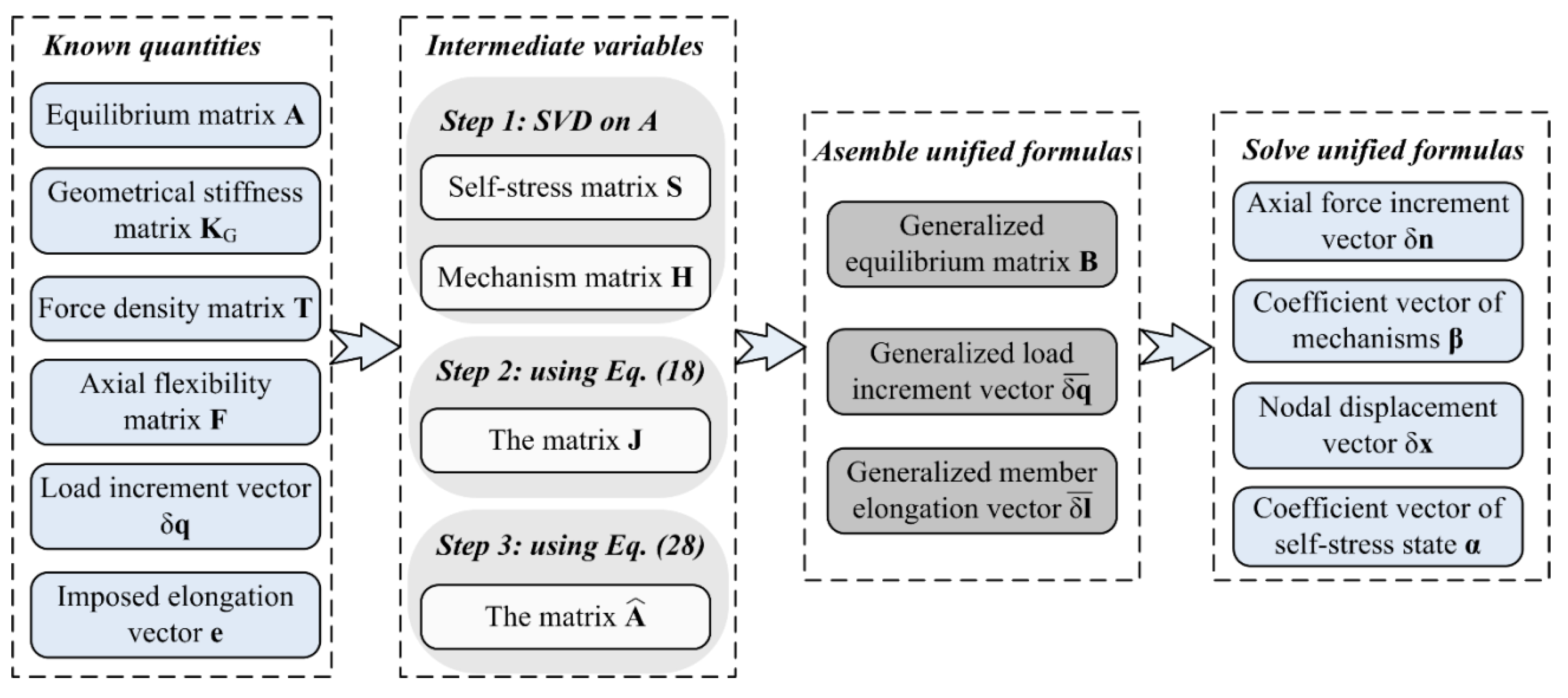Particularly, when Equations (41) and (42) are used for type I assemblies, the matrix B is reduced to A, while $\overline{\mathsf{\delta }\mathbf{q}}$ and $\overline{\mathsf{\delta }\mathbf{L}}$ degenerate into δq and δl, respectively. Therefore, they can be regarded as generalized equilibrium equations and compatibility equations implying constitutive relations. Since the derivation of Equations (41) and (42) does not involve the unique properties of type IV assemblies, they are applicable to types I, II, and III assemblies as well. In order to facilitate the readers to follow the above derivation process, Figure 1 gives a road map for development of the unified formulas presented in this section, while Figure 2 shows the calculation steps to guide the designers to apply the proposed formulas.

Figure 1. Road map for derivation of the unified formulas.

Figure 2. Calculation procedure of applying the unified formulas.

4. Comparison with Other Formulations

4.1. Matrix Force Method

Pellegrino and Calladine [4,14] proposed a matrix analysis method based on the concept of force method, which is used for statically and kinematically indeterminate assemblies. This section will discuss the similarities and differences between that method and the method proposed in this paper.

As described in Section 2, starting from Equation (22), δx can be regarded as the basic unknown variable of the system. When the consistent condition given by Equation (23) is satisfied, δx can be solved form Equation (24). Furthermore, δx may be divided as follows:

$$\mathsf{\delta }\mathbf{x}=\underset{\mathsf{\delta }{\mathbf{x}}^{\mathrm{I}}}{\underbrace{{({\mathbf{A}}^{\mathrm{T}})}^{+}(\mathbf{e}+\mathbf{F}·\mathsf{\delta }\mathbf{n})+\mathbf{H}{\mathsf{\beta }}^{\mathrm{I}}}}+\underset{\mathsf{\delta }{\mathbf{x}}^{\mathrm{II}}}{\underbrace{\mathbf{H}{\mathsf{\beta }}^{\mathrm{II}}}}$$

(43)

where β^I and β^II are the vectors that need to be determined further, satisfying β^I + β^II = β. In Equation (43), δx^I related to the elastic elongations of the bars is called ‘extensional deformation’, while δx^II only associated with the infinitesimal mechanism corresponds to ‘inextensional deformation’ [14].

Next, the incremental form of equilibrium equations given by Equation (19)—Aδn + Jδx = δq—is investigated. As mentioned before, the second item on the left side of Equation (19) represents the resistance arising from small nodal displacements when the internal forces of the bars are kept constant. Thus, they are called “product forces” in Pellegrino and Calladine [14]. If the product forces caused by δx^I are ignored and the relations given by Equation (29) (JH = K_GH) are considered, Equation (19) can be rewritten as:

$$\mathbf{A}·\mathsf{\delta }\mathbf{n}+{\mathbf{K}}_G\mathbf{H}{\mathsf{\beta }}^{\mathrm{II}}=\mathsf{\delta }\mathbf{q}$$

(44)

Equation (44) can be combined with the existence condition given by Equation (23), assembled in matrix form as:

$$\left[\begin{array}{cc}\mathbf{A}& {\mathbf{K}}_G\mathbf{H}\\ -{\mathbf{S}}^{\mathrm{T}}\mathbf{F}& \mathbf{0}\end{array}\right]\left(\begin{array}{c}\mathsf{\delta }\mathbf{n}\\ {\mathsf{\beta }}^{\mathrm{II}}\end{array}\right)=\left(\begin{array}{c}\mathsf{\delta }\mathbf{q}\\ {\mathbf{S}}^{\mathrm{T}}\mathbf{e}\end{array}\right)$$

(45)

from which δn and β^II can be obtained.

Finally, the solution of β^I (or δx^I) will be determined. From the compatibility Equation (21), we can see that ${\mathbf{A}}^{\mathrm{T}}(\mathsf{\delta }{\mathbf{x}}^{\mathrm{I}}+\mathsf{\delta }{\mathbf{x}}^{\mathrm{II}})=\mathbf{e}+\mathbf{F}·\mathsf{\delta }\mathbf{n}$ holds. Because of ${\mathbf{A}}^{\mathrm{T}}\mathsf{\delta }{\mathbf{x}}^{\mathrm{II}}={\mathbf{A}}^{\mathrm{T}}\mathbf{H}{\mathsf{\beta }}^{\mathrm{II}}=0$, the following formula is obtained

$${\mathbf{A}}^{\mathrm{T}}\mathsf{\delta }{\mathbf{x}}^{\mathrm{I}}=\mathbf{e}+\mathbf{F}·\mathsf{\delta }\mathbf{n}$$

(46)

For kinematically indeterminate structures, Equation (46) possesses infinite solutions, that is to say, β^I is optional. In order to determine the unique β^I, the new constraint conditions have to be considered further.

The two sides of Equation (44) are left multiplied by H^T simultaneously:

$${\mathbf{H}}^{\mathrm{T}}{\mathbf{K}}_G\mathbf{H}{\mathsf{\beta }}^{\mathrm{II}}={\mathbf{H}}^{\mathrm{T}}\mathsf{\delta }\mathbf{q}$$

(47)

Note that δx satisfies Equation (35), i.e.,

$${\mathbf{H}}^{\mathrm{T}}{\mathbf{K}}_G·(\mathsf{\delta }{\mathbf{x}}^{\mathrm{I}}+\mathbf{H}{\mathsf{\beta }}^{\mathrm{II}})={\mathbf{H}}^{\mathrm{T}}·\mathsf{\delta }\mathbf{q}$$

(48)

Then, the subtraction of Equation (47) form Equation (48) yields

$${\mathbf{H}}^{\mathrm{T}}{\mathbf{K}}_G\mathsf{\delta }{\mathbf{x}}^{\mathrm{I}}={({\mathbf{K}}_G\mathbf{H})}^{\mathrm{T}}\mathsf{\delta }{\mathbf{x}}^{\mathrm{I}}=\mathbf{0}$$

(49)

where the matrix K_GH is made up of product-force vectors arranged in columns (it is consistent with the constraint equations derived from the principle of virtual work in Pellegrino and Calladine [14]). Then, Equations (49) and (46) are combined and written in the following matrix form:

$${\left[\begin{array}{cc}\mathbf{A}& {\mathbf{K}}_G\mathbf{H}\end{array}\right]}^{\mathrm{T}}\mathsf{\delta }{\mathbf{x}}^{\mathrm{I}}=\left(\begin{array}{c}\mathbf{e}+\mathbf{F}·\mathsf{\delta }\mathbf{n}\\ \mathbf{0}\end{array}\right)$$

(50)

from which δx^I can be obtained.

The matrix analysis algorithm based on traditional force method, proposed in Pellegrino and Calladine [14], can be described by the fundamental formulas composed of Equations (45) and (50) in essence. For convenience, it is called “matrix force method” in this paper. It can be seen from the above discussions that, the matrix force method is applicable to the situation where the product forces caused by extensional deformation δx^I can be ignored. Specifically, it can be divided into two situations: (1) the absolute values of the product forces caused by δx^I are small enough; (2) the values of the product forces caused by δx^I are relatively small compared with the ones resulting from δx^II. It is worth mentioning that the type IV assembles—statically and kinematically indeterminate ones—usually belong to the latter situation. Therefore, the static analysis results obtained from the two methods are often close to each other. Although the fundamental formulas proposed in this paper are more complex than the ones of the matrix force method, they are applicable to static analysis of a general pin-jointed assembly based on the assumption of small deformation and linear elasticity, which will be further verified through several numerical examples in the next section.

4.2. Displacement-Based Method

To derive Equation (41), the variable δn was employed to express δx from Equation (21) in Section 3. When A is a rectangular matrix and does not have full row rank, the expression of the general solution of δx includes the generalized inverse of A and the matrix H consisting of a full basis for the left nullspace of A (see Equation (24)). Meanwhile, the consistent condition to ensure the existence of the solutions of δx in Equation (21) arises, given by Equation (23). However, if the variable δx is employed to express δn from Equation (21), the expression is much simpler as:

$$\mathsf{\delta }\mathbf{n}=\mathbf{G}({\mathbf{A}}^{\mathrm{T}}\mathsf{\delta }\mathbf{x}-\mathbf{e})$$

(51)

where G = F⁻¹ is called as axial stiffness matrix of bars. Substitute Equation (51) into Equation (19) and tidy up:

$$\mathbf{A}\widehat{\mathbf{G}}{\mathbf{A}}^{\mathrm{T}}·\mathsf{\delta }\mathbf{x}+{\mathbf{K}}_{\mathbf{G}}·\mathsf{\delta }\mathbf{x}=\mathsf{\delta }\mathbf{q}+\mathbf{A}\mathbf{G}\mathbf{e}$$

(52)

where $\widehat{\mathbf{G}}=\mathbf{G}-\mathrm{T}$ is the diagonal matrix. The matrix $\mathbf{A}\widehat{\mathbf{G}}{\mathbf{A}}^{\mathrm{T}}$ is usually called elastic stiffness matrix, denoted by K_E. Then Equation (52) can be further written as:

$$({\mathbf{K}}_E+{\mathbf{K}}_G)·\mathsf{\delta }\mathbf{x}=\mathbf{K}·\mathsf{\delta }\mathbf{x}=\mathsf{\delta }\mathbf{q}+\mathbf{A}\mathbf{G}\mathbf{e}$$

(53)

where K is the so-called tangent stiffness matrix of the structure.

Equation (53) is the fundamental formula of the matrix displacement method, and its iterative procedures to deal with nonlinear problems are as follows: (1) assemble the tangent stiffness matrix of the structure—K; (2) make use of Equation (53) to calculate the nodal displacements in step i—δxⁱ; (3) update the nodal coordinates in terms of δxⁱ; (4) assemble the tangent stiffness matrix and the unbalanced nodal loads vector based on the new configuration; (5) substitute them into Equation (53) to calculate the nodal displacements in step i + 1—δxⁱ⁺¹. Repeat the above procedures until the nodal displacements or the unbalanced nodal loads are small enough to satisfy the preset accuracy requirements.

It should be noted that the matrix displacement method is regarded as a benchmark in this paper to test the accuracy and applicability of the other two force methods mentioned above, since it can achieve a high precision by running iterative schemes.

5. Numerical Examples

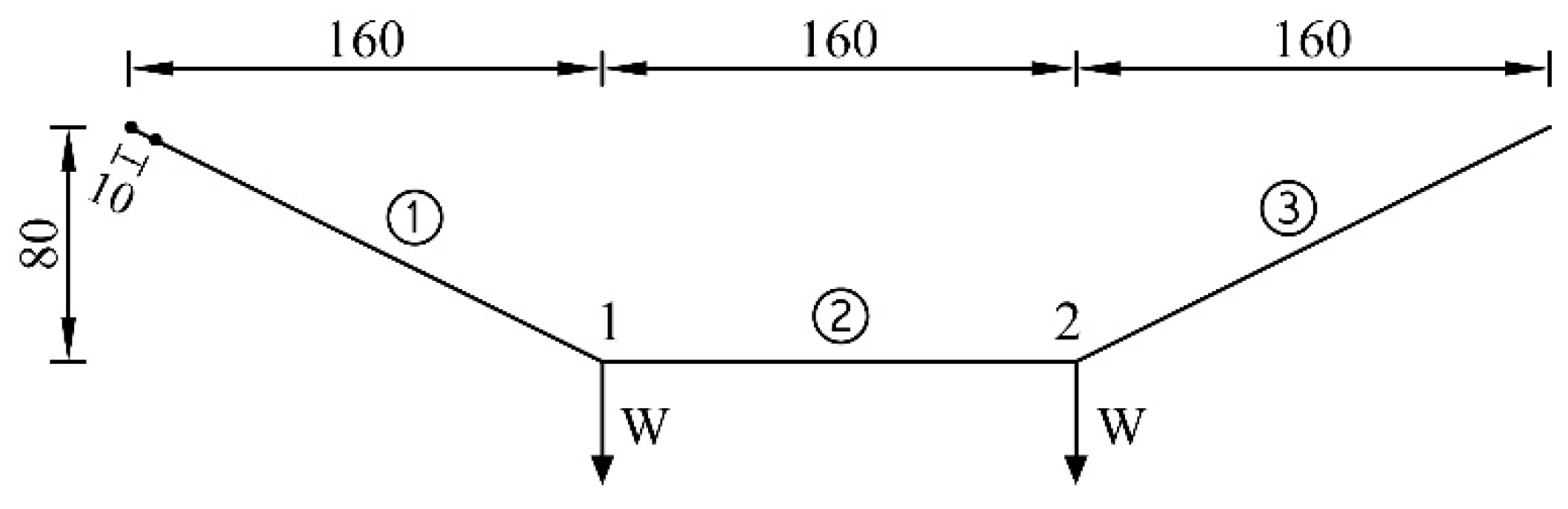
Example 1 [4] Figure 3 shows a planar hanging cable with three segments under concentrated loads. The product of Young’s modulus and the cross-section area of the cable satisfies EA = 1.836 × 10⁴ N. Two equal weights were hung as shown in Figure 3. All dimensions are in mm. Consider the situation that the cable segment 1 is shortened by 10 mm (it is obtained by letting 10 mm of cable slide through the left-hand pin), while the lengths of cable segments 2 and 3 are fixed. How to determine the final configurations when W = 30 N and W = 3000 N are imposed, respectively?

Figure 3. A planar hanging cable with three segments under concentrated loads (mm).

The system of equilibrium Equation (1) for this assembly is

$$\mathbf{A}\mathbf{n}=\mathbf{q}\Rightarrow$$

$$\left[\begin{array}{ccc}0.8944& -1& 0\\ 0.4472& 0& 0\\ 0& 1& -0.8944\\ 0& 0& 0.4472\end{array}\right]\left(\begin{array}{c}{\mathrm{n}}_1\\ {\mathrm{n}}_2\\ {\mathrm{n}}_3\end{array}\right)=\left(\begin{array}{c}0\\ \mathrm{W}\\ 0\\ \mathrm{W}\end{array}\right)$$

The rank of A is 3. Hence, the numbers of independent mechanisms and self-stress states are m = 1 and s = 0 respectively, which means that this system belongs to type III—statically determinate and kinematically indeterminate assemblies. The unique mechanism composing the matrix H can be obtained by Singular Value Decomposition of the matrix A, which is normalized as:

$$\mathbf{H}={[0.3162-0.63250.31620.6325]}^{\mathrm{T}}$$

The initial axial forces of the cable segments are solved from the equilibrium equations:

$$\mathbf{n}={\mathbf{A}}^{+}\mathbf{q}=\left(\begin{array}{c}2.236\mathrm{W}\\ 2\mathrm{W}\\ 2.236\mathrm{W}\end{array}\right)$$

Then, the force density vector can be calculated further:

$$\mathbf{t}={\mathbf{L}}^{-1}\mathbf{n}=0.0125\mathrm{W}{[111]}^{\mathrm{T}}$$

K_G is obtained from the following formula:

$${\mathbf{K}}_{\mathrm{G}}=\left[\begin{array}{cc}{\mathrm{t}}_1+{\mathrm{t}}_2& -{\mathrm{t}}_2\\ -{\mathrm{t}}_2& {\mathrm{t}}_2+{\mathrm{t}}_3\end{array}\right]\otimes {\mathbf{I}}_{2\times 2}$$

Thus

$${\mathbf{K}}_{\mathrm{G}}\mathbf{H}=0.003953\mathrm{W}{[-16-1-6]}^{\mathrm{T}}$$

A, T, and K_G are substituted into Equation (18) to get the matrix J. The axial flexibility matrix F is also assembled. Then the matrix $\widehat{\mathbf{A}}$ can be obtained by substituting F and J into Equation (28).

When W = 30 N holds, the generalized equilibrium matrix B can be obtained from Equation (40):

$$\mathbf{B}=[\widehat{\mathbf{A}}{\mathbf{K}}_{\mathrm{G}}\mathbf{H}]\Rightarrow$$

$$\mathbf{B}=\left[\begin{array}{ccc}0.8928& -1.0016& -0.0016\\ 0.4521& 0.0033& 0.0016\\ 0.0016& 1.0016& -0.8928\\ 0.0016& 0.0033& 0.4521\end{array}|\begin{array}{c}0.1186\\ -0.7115\\ 0.1186\\ 0.7115\end{array}\right]$$

It is easy to verify that the matrix B has full rank, and the initial nodal loads vector q is orthogonal to the mechanism H. In other words, the mechanism is stiffened by the external loads. The system becomes a relatively stable structure that can withstand the external disturbance.

Consider that the cable segment 1 is shortened by 10 mm, i.e., the imposed elongation vector satisfies e = [−10 0 0]^T, while the increments of the nodal loads satisfy δq = 0. The generalized nodal loads vector (incremental form) and bar elongation vector are given as:

$$\overline{\mathsf{\delta }\mathbf{q}}=\mathsf{\delta }\mathbf{q}-\mathbf{J}{({\mathbf{A}}^{+})}^{\mathrm{T}}\mathbf{e}={[-1.685.031.681.68]}^T$$

$$\overline{\mathsf{\delta }\mathbf{l}}=\left(\begin{array}{c}\mathbf{F}{\mathbf{A}}^{+}\mathsf{\delta }\mathbf{q}+\mathbf{e}\\ {\mathbf{H}}^{\mathrm{T}}·\mathsf{\delta }\mathbf{q}\end{array}\right)={[-10000]}^{\mathrm{T}}$$

Then, the following solutions are derived from Equations (41) and (42), respectively

$$\overline{\mathsf{\delta }\mathbf{n}}=\left(\begin{array}{c}\mathsf{\delta }\mathbf{n}\\ \mathsf{\beta }\end{array}\right)={\mathbf{B}}^{-1}\overline{\mathsf{\delta }\mathbf{q}}=\left(\begin{array}{c}7.6212\\ 8.1985\\ 7.0446\\ -2.1745\end{array}\right)$$

and

$$\overline{\mathsf{\delta }\mathbf{x}}=\mathsf{\delta }\mathbf{x}={({\mathbf{B}}^{\mathrm{T}})}^{-1}\overline{\mathsf{\delta }\mathbf{l}}\Rightarrow$$

$$\mathsf{\delta }\mathbf{x}={[-5.1930-11.8087-5.1215-10.0896]}^{\mathrm{T}}$$

Similarly, the static analysis can be performed for the case of W = 3000 N through the same algorithm as described above. In addition, the fundamental formulas of the so-called matrix force method (see Section 4.2) and the iterative schemes of the matrix displacement method (see Section 4.1) are also employed to solve the same problem (the latter is implemented in Matlab 7.0 (R14) software, and its calculation results are regarded as a standard herein). For simplicity, Methods 1, 2, and 3 are used to represent the method proposed in this paper, the matrix force method, and the nonlinear matrix displacement method respectively. The axial forces of members and the displacements of nodes are listed in Table 2 and Table 3.

Table 2. Axial forces of members in Example 1 (N).

W	Cable Segments	n (Initial Axial Force)	δn (the Increments of n)
			Method 1	Error (%)	Method 2	Error (%)	Method 3
W = 30	①	67.08	7.621	−19.192	0	−100	9.431
	②	60.00	8.199	−18.902	0	−100	10.113
	③	67.08	7.045	−21.082	0	−100	8.927
W = 3000	①	6708	256.076	−1.424	0	−100	259.778
	②	6000	255.767	−1.578	0	−100	259.930
	③	6708	201.454	−2.657	0	−100	207.046

Table 3. Displacements of nodes in Example 1 (mm).

W	Nodes	Directions	Method 1	Error (%)	Method 2	Error (%)	Method 3
W = 30 N	1	x-direction	−5.193	0.562	−5.160	−0.077	−5.164
		y-direction	−11.809	−4.217	−12.040	−2.352	−12.332
	2	x-direction	−5.122	0.787	−5.160	1.535	−5.082
		y-direction	−10.090	−7.176	−10.320	−5.060	−10.870
W = 3000 N	1	x-direction	−6.000	−0.150	−5.160	−14.129	−6.009
		y-direction	−4.782	1.810	−12.040	156.334	−4.697
	2	x-direction	−3.771	0.506	−5.160	37.527	−3.752
		y-direction	−3.153	1.187	−10.320	231.194	−3.116

It has been found that when the initial external load W is small (e.g., W = 30 N), the nodal displacements solved by both Method 1 and Method 2 are comparable, and approximate the numerical solutions obtained from Method 3 considering the geometric nonlinearity. When W becomes large (e.g., W = 3000 N), the errors using Method 2 increase dramatically, whereas the results obtained from Method 1 even fit better with the numerical solutions—the maximum error is only 1.81% in comparison with 7.18% when W = 30 N. Understandably, the increment of W will increase the initial axial forces of members, which will strengthen the rigidity of the structure, which will weaken the nonlinearity of the structure. Hence, the errors using Method 1 decrease when W becomes large.

It is also interesting to note that Method 2 gives the same calculation results for both situations of W = 30 N and W = 3000 N. The reason is that, to deal with type III assemblies, one of the fundamental equations of Method 2—Equation (45)—is reduced to:

$$\left[\begin{array}{cc}\mathbf{A}& {\mathbf{K}}_G\mathbf{H}\end{array}\right]\left(\begin{array}{c}\mathsf{\delta }\mathbf{n}\\ {\mathsf{\beta }}^{\mathrm{II}}\end{array}\right)=\mathsf{\delta }\mathbf{q}$$

Since δq = 0 holds in this example, we can get the solutions of δn = 0 and β^II = 0 (i.e., δx = δx^I) from the above formula, substituting which into Equation (50) gives

$${\left[\begin{array}{cc}\mathbf{A}& {\mathbf{K}}_G\mathbf{H}\end{array}\right]}^{\mathrm{T}}\mathsf{\delta }\mathbf{x}=\left(\begin{array}{c}\mathbf{e}\\ 0\end{array}\right)$$

As observed, δx solved from the above formula is irrelevant to the initial nodal load W.

In fact, when the value of W is small, it only plays a role of tightening the cable segments, and the elastic deformation caused by W can be ignored. In this case, the calculation model of the system is simplified as a mechanism composed of three rigid bars, as shown in Figure 4. Therefore, a 10-mm shortening of cable segment 1 only results in nodal displacements and causes no axial force in the cable. The solutions derived from the matrix force method correspond to this situation. However, when the value of W is large, the effect of preventing the cable segment 1 shortened has to be taken into account, which will definitely cause the elastic deformation of the cable segments. Hence, the simplified model shown in Figure 4 cannot be employed, and the matrix force method is no longer applicable.

Figure 4. The simplified calculation model for the case of W = 30 N.

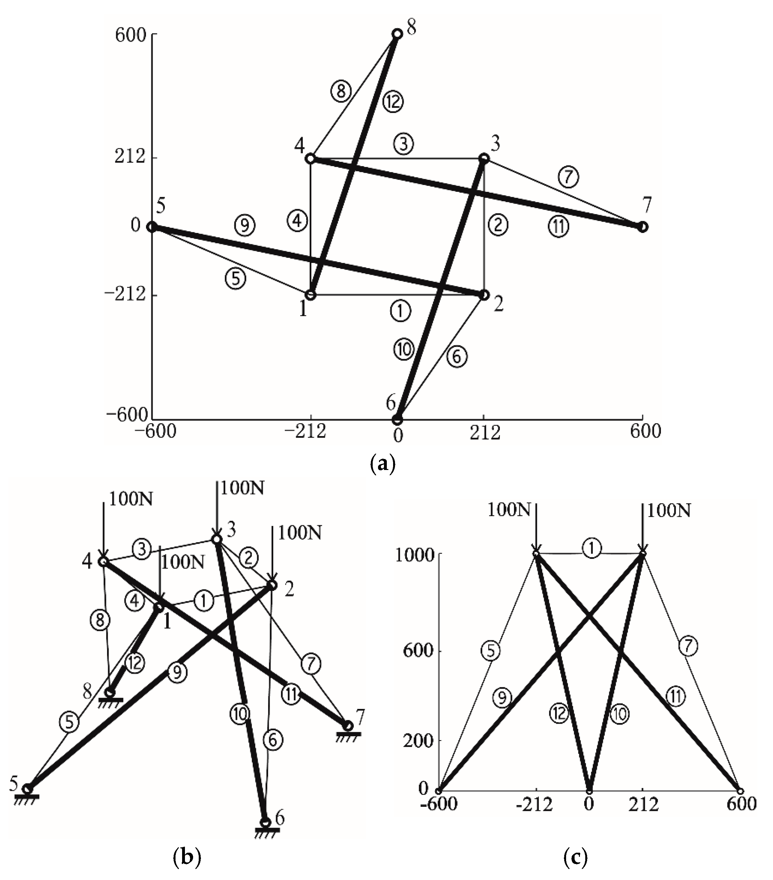
Example 2 Figure 5 shows a prestressed cable-strut structure composed of 4 struts (drawn by thick lines) and 8 cables (drawn by thin lines). It possesses 8 nodes, in which the four upper nodes are free and the four lower ones are pin-jointed with the ground. Hence, the nodal degree of freedom of the system d is equal to 12. The rank of equilibrium matrix A is 11. Hence, the numbers of independent mechanisms and self-stress states are m = 1 and s = 1 respectively, which means that this system belongs to type IV—statically and kinematically indeterminate assemblies. The mechanism of this structure can be stiffened by introducing a certain amount of prestress. In this example, the prestress state can be determined by multiplying the unique normalized self-stress state by a coefficient μ, so that μ represents the level of prestress. Assume that μ = 8000 N holds. Meanwhile, the products of Young’s modulus and the cross-section area for cables and struts satisfy (EA)_cable = 1.836 × 10⁴ N and (EA)_strut = 5.796 × 10⁶N. Let us consider the following two situations respectively:

Figure 5. A prestressed cable-strut structure with 4 struts and 8 cables. (a) Top view (mm); (b) perspective view; (c) side view (mm).

Situation 1: the vertical concentrated loads are applied on the four upper nodes, as shown in Figure 5b.

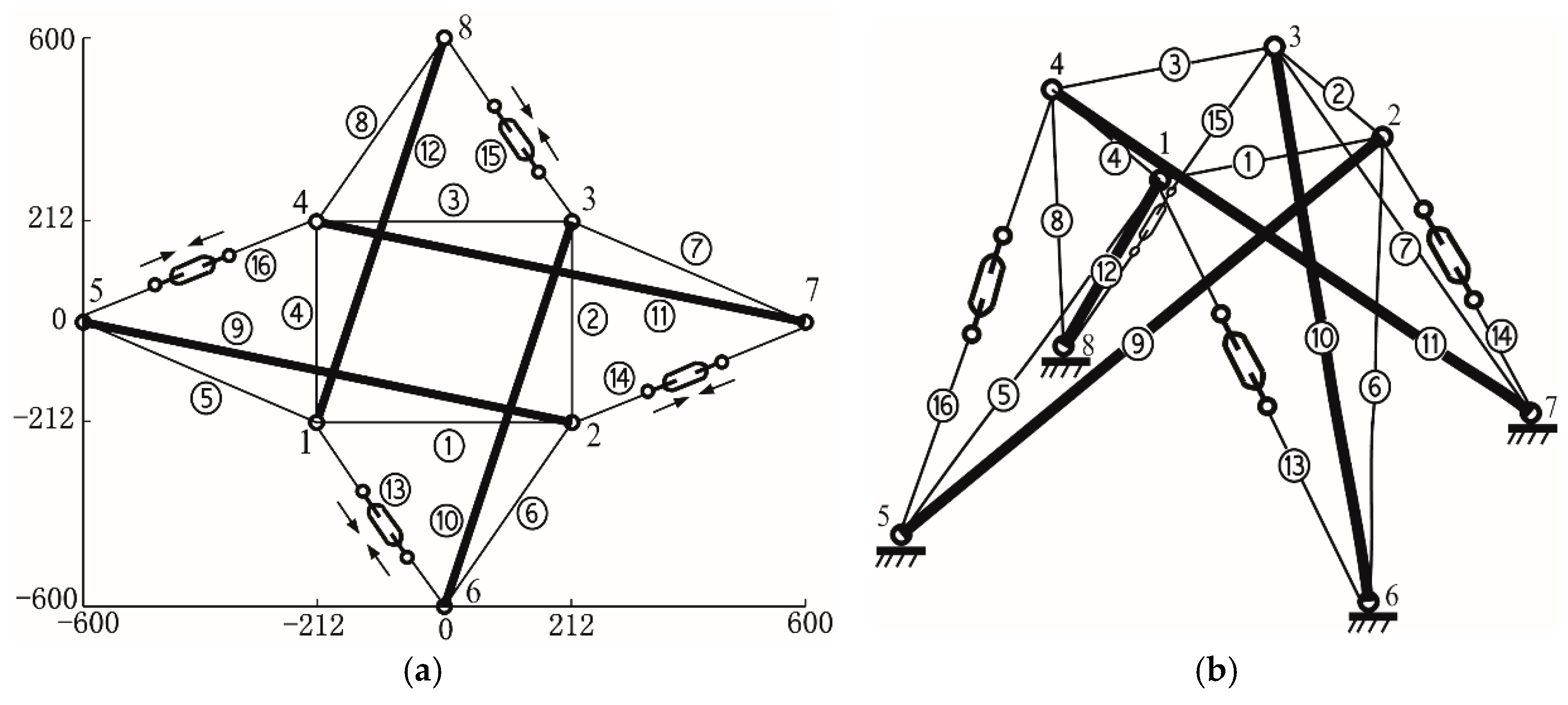
Situation 2: four cables are added to connect certain pairs of nodes, as shown in Figure 6. The added cables are assumed to be adjustable by embedding the turnbuckles, and they are shortened by 10 mm synchronously. It should be noted that the type of the structure has been changed after the increments of cables. Although the nodal degree of freedom d is still equal to 12, the number of elements b becomes 16 and the rank of new equilibrium matrix A is 12. Therefore, s = 4 and m = 0 hold, which means that this system belongs to type II—statically indeterminate and kinematically determinate assemblies.

Figure 6. A prestressed cable-strut structure with 4 struts and 12 cables (the lengths of 4 added cables are adjustable). (a) Top view (mm); (b) perspective view.

The static analyses are carried out for the above two situations, using aforementioned three methods respectively. The calculation results are listed in Table 4 and Table 5. It should be noted that the structure discussed herein satisfies the invariance condition to rotation around the vertical axis by a certain degree. Accordingly, the members can be divided into four groups totally, i.e., horizontal cables numbered from ① to ④, vertical cables numbered from ⑤ to ⑧, struts numbered from ⑨ to ⑫, added cables numbered from ⑬ to ⑯, because all members in each group are located at symmetrical positions—one member in each group can be transformed to any other member of that group by a proper rotational operation. Similarly, four free nodes numbered from 1 to 4 are also located at symmetrical positions, according to the rotational symmetric property of the structure. Thus, we just need to focus on the displacement results of Node 1.

Table 4. Axial force of members in Example 2 (N).

Situations	Members	n (Initial Axial Force)	δn (the Increments of n)
			Method 1	Error (%)	Method 2	Error (%)	Method 3
1	① to ④	1311.3	46.254	−1.996	45.592	−3.398	47.196
	⑤ to ⑧	2389.5	−10.390	8.173	−10.243	6.641	−9.605
	⑨ to ⑫	−2853.3	−119.708	−1.039	−118.328	−2.180	−120.965
2	① to ④	1311.3	30.325	−4.869	0	−100	31.877
	⑤ to ⑧	2389.5	−6.755	15.946	0	−100	−5.826
	⑨ to ⑫	−2853.3	−65.954	−3.548	0	−100	−68.380
	⑬ to ⑯	0	61.137	−1.397	0	−100	62.003

Table 5. Displacements of Node 1 in Example 2 (mm).

Situations	Directions	Method 1	Error (%)	Method 2	Error (%)	Method 3
1	x-direction	4.319	0.512	4.327	0.698	4.297
	y-direction	−5.388	2.045	−5.380	1.894	−5.280
	z-direction	−3.495	1.569	−3.486	1.308	−3.441
2	x-direction	5.077	−0.743	9.111	78.123	5.115
	y-direction	−5.778	1.120	−9.111	59.450	−5.714
	z-direction	−3.635	0.665	−5.467	51.399	−3.611

It can be seen from the above two tables that for the first situation, the solutions of axial forces and displacements obtained from both Method 1 and Method 2 almost have the same level of error, and approximate the numerical solutions derived from Method 3 considering the geometric nonlinearity. For the second situation, the results given by Method 1 are still in good agreement with the numerical solutions, whereas the results derived from Method 2 are quite different from them. The reason is that, in the first situation, the product forces caused by δx^I are relatively small compared with the ones resulting from δx^II and, therefore, considering (like Method 1) or ignoring (like Method 2) the contribution of this part has little effect on the final results. However, when Method 2 is employed to deal with type II assemblies in the second situation, the fundamental Equations (45) and (50) are reduced to:

$$\left(\begin{array}{c}\mathbf{A}\\ -{\mathbf{S}}^{\mathrm{T}}\mathbf{F}\end{array}\right)\mathsf{\delta }\mathbf{n}=\left(\begin{array}{c}\mathsf{\delta }\mathbf{q}\\ {\mathbf{S}}^{\mathrm{T}}\mathbf{e}\end{array}\right)$$

and

$${\mathbf{A}}^{\mathrm{T}}\mathsf{\delta }\mathbf{x}=\mathbf{e}+\mathbf{F}·\mathsf{\delta }\mathbf{n}$$

Actually, the above two formulas are the fundamental equations of traditional force method used for type II assemblies, which cannot consider the influence of initial axial forces or prestress. Therefore, the results obtained from Method 2 are irrelevant to prestress, and their calculation errors will become larger with the increase of prestress level μ. Fortunately, this inherent flaw for Method 2 has been improved in Method 1 since no redundant simplifications were made in the derivation of the unified formulas.

As to the second situation of this example, four independent states of self-stress S_i (i = 1, 2, 3, 4) can be obtained through the Singular Value Decomposition of the equilibrium matrix, each of which is formed as:

$${\mathbf{S}}_{\mathrm{i}}={[{\mathrm{s}}_{\mathrm{i}}^1\cdots {\mathrm{s}}_{\mathrm{i}}^{12}{\mathrm{s}}_{\mathrm{i}}^{13}\cdots {\mathrm{s}}_{\mathrm{i}}^{16}]}^{\mathrm{T}}$$

Among 16 entries of S_i, the first 12 ones correspond to the original 12 members, while the last 4 ones correspond to the 4 added cables. It is found that S_i is featured by the fact that the sum of the last 4 entries is zero, i.e., the following equation holds

$${\displaystyle \sum _{j=13}^{16}{\mathrm{s}}_{\mathrm{i}}^j}=0$$

Because of $\mathbf{e}={[\underset{12}{\underbrace{0\cdots 0}}\underset{4}{\underbrace{-10\cdots -10}}]}^T$, the equation S^Te = 0 holds. Moreover, due to δq = 0, then:

$$\left(\begin{array}{c}\mathsf{\delta }\mathbf{q}\\ {\mathbf{S}}^{\mathrm{T}}{\mathbf{e}}_0\end{array}\right)=0$$

From the reduced forms of Equations (45) and (50), we can get the solutions of δn = 0 and $\mathsf{\delta }\mathbf{x}={({\mathbf{A}}^{\mathrm{T}})}^{+}(\mathbf{e}+\mathbf{F}·\mathsf{\delta }\mathbf{n})={(\mathbf{A}{\mathbf{A}}^{\mathrm{T}})}^{-1}\mathbf{A}·\mathbf{e}$, which will keep unchanged with the variation of the prestress level μ.

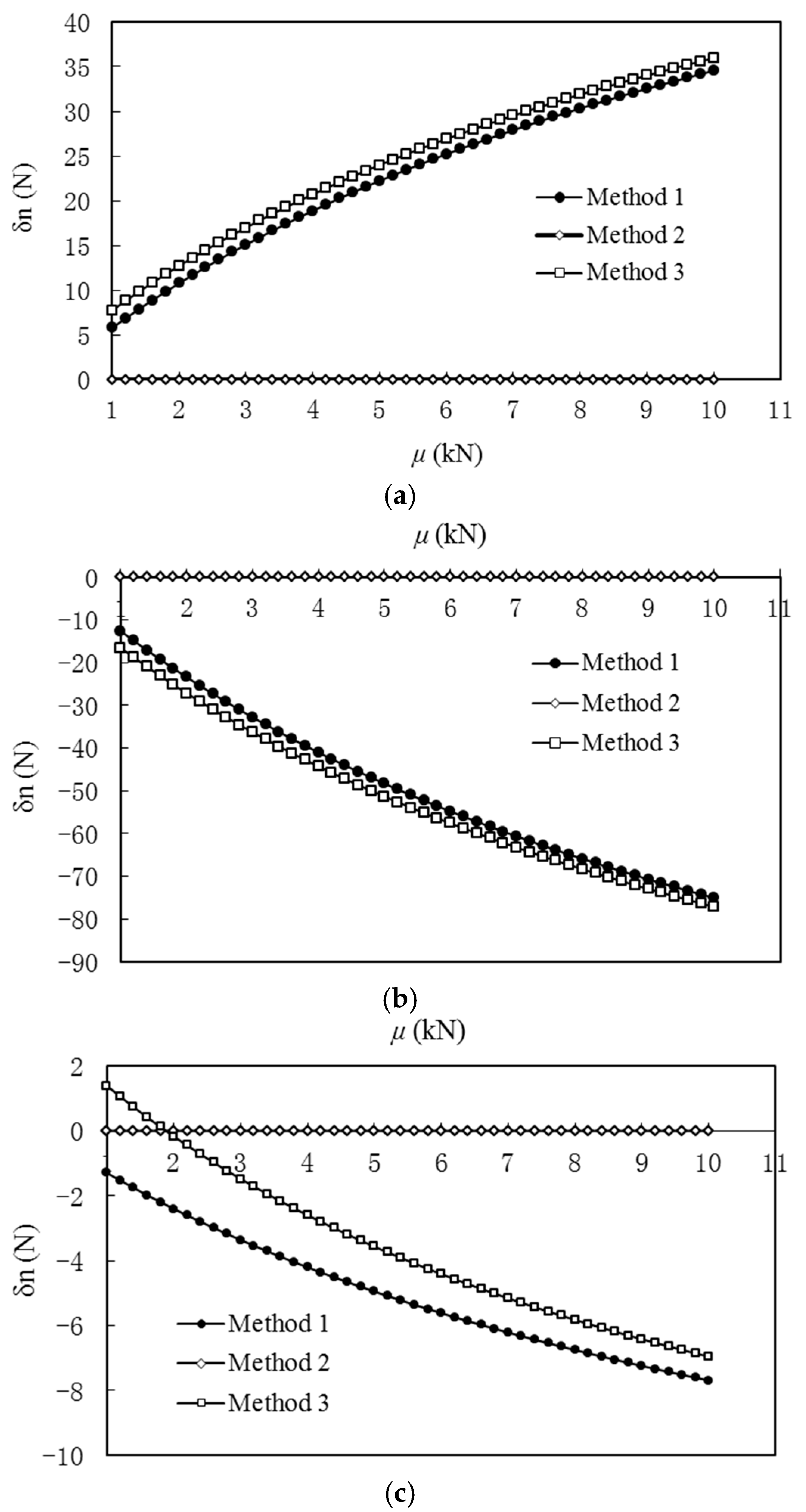
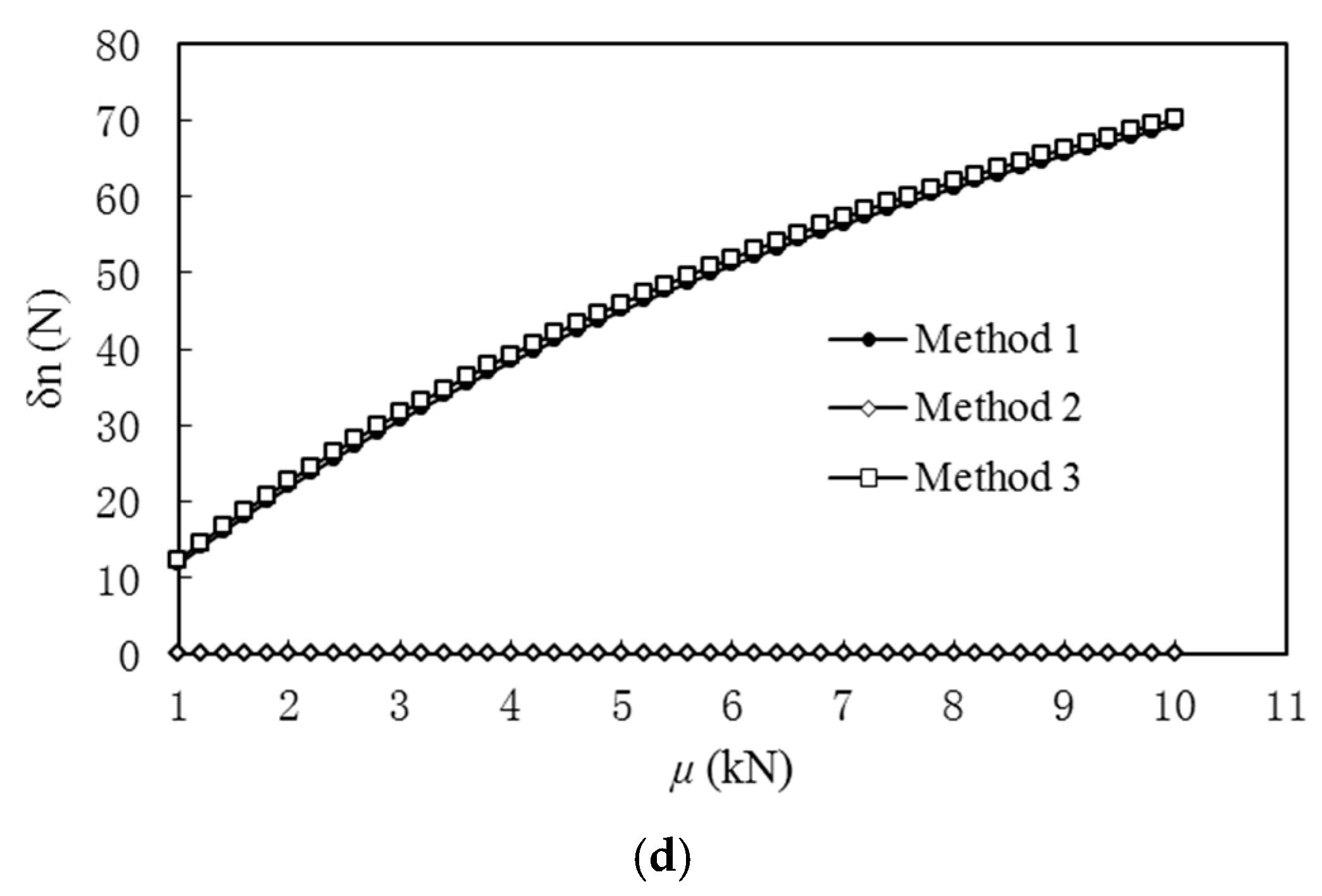
To verify the above arguments, considering that μ is raised from 1 kN to 10 kN, the increments of the axial forces of the members are calculated for Situation 2 using the aforementioned three methods, respectively, the results of which are shown in Figure 7. It can be seen from this figure that the solutions derived from the matrix force method are always equal to zeros, which deviate from the numerical solutions gradually with the increase of μ. On the other hand, the method proposed in this paper is in a good agreement with the nonlinear matrix displacement method. Furthermore, the larger the initial axial forces are, the greater the structural stiffness is, the lower the nonlinearity is, and the higher the accuracy is.

Figure 7. The increments of axial forces δn with respect to different levels of prestress μ. (a) The members numbered from ① to ④; (b) the members numbered from ⑤ to ⑧; (c) the members numbered from ⑨ to ⑫; (d) the members numbered from ⑬ to ⑯.

6. Conclusions

(1) The fundamental formulas of the static analysis of the pin-jointed bar assemblies, considering the influence of initial axial forces of members, are derived based on the assumption of small deformation and linear elasticity, which consist of the generalized equilibrium equations and the generalized compatibility equations. They are consistent with the fundamental formulas of the traditional force method for type I—statically and kinematically determinate structures in the form, because both the system of generalized equilibrium equations and that of compatibility equations have square coefficient matrices of full rank being transposed with each other. Particularly, they reduce to the fundamental formulas of the traditional force method when they are applied to type I assemblies. Therefore, the theory presented in this paper can be regarded as a direct extension of the traditional force method, considering the influence of initial axial forces of the bars.

(2) In comparison with the displacement-based algorithm, the proposed method has its own advantages—the physical concepts of each item in equations are fairly explicit. The combination coefficients of self-stress states and mechanisms are obtained at the same time of solving the structural responses, which is very helpful for us to essentially comprehend the mechanism of resisting external loads for pin-jointed bar assemblies. The theoretical analysis and numerical examples show that the fundamental formulas given in this paper possesses a wider scope of applications than those of the “matrix force method” presented by Pellegrino and Calladine [4,14], although they are more complex in form.

(3) Since the theory presented in this paper is based on the singular value decomposition and the generalized inverse matrix, it is not suitable for iterative procedures. Therefore, the nonlinear matrix displacement method or the finite element method cannot be replaced for structures with the strong geometric nonlinearity.