Analysis of an Optical Lattice Methodology for Detection of Atomic Parity Nonconservation

Abstract

We present an extension and a deepened analysis of a suggested experimental scheme for detecting atomic parity violation, previously published in Phys. Rev. A 2019, 100, 050101. The experimental concept is described in more detail and we compute new ab initio data necessary for assessing the plausibility of the approach. Original theoretical data for transition matrix elements on the electric dipole forbidden transition in caesium $6\mathrm{s}{}^2{\mathrm{S}}_{1/2}$–$5\mathrm{d}{}^2{\mathrm{D}}_{3/2}$ are reported, as are a range of electric dipole matrix elements connected to the ground state 6s. The latter is used for an analysis of the wavelength-dependent light shift in Cs. A range of experimental details is presented, combined with a survey of realistic lasers parameters. These are adopted to project the feasibility of the scheme to eventually be capable of delivering data beyond the standard model of particle physics.

1. Introduction

The role of symmetry is central in the standard model (SM) of elementary particle physics [1,2]. The argument that a symmetric conservation law may not apply to the parity of the wave functions of physical systems was published in 1956 by Tsung-Dao Lee and Chen-Ning Yang [3]. In the following year, clear experimental proofs of parity violation were reported by Chien-Shiung Wu and her group [4].

While parity non-conservation (PNC) has frequently been studied at high energies (see e.g., [5]), the opportunity of using atomic or molecular systems for experimental surveys at the other end of the energy spectrum was introduced by Bouchiat and Bouchiat [6,7]. The week interaction was predicted to have a subtle influence on atomic spectra, and with a carefully designed high-precision experiment, combined with leading-edge theoretical computations of atomic parameters, such studies constitute tests of the SM.

The effect is very subtle. For light and medium-size atomic species, they are well beyond being possible to detect by current spectroscopic technology. However, the influence of PNC effects increases rapidly for increasing nuclear mass, at least as $Z^3$ (with Z the atomic number) [6]. For heavy atoms, the feasibility for detection is still difficult, but not entirely excluded.

Heavy atoms, however, carry the drawback that atomic ab initio calculations, crucial for the interpretation of the results, are more difficult for large Z because of the increased importance of relativistic effects. For this reason, many experimental attempts, or suggestions, to observe atomic PNC employ alkali atoms or the isoelectronic ions. The sole valence electron greatly facilitates exact computations, and at the same time, the relatively simple energy level spectra of alkalis also imply considerable experimental advantages.

In the context of atomic spectra, the way in which the parity violation shows up can be divided into two categories (see e.g., [8,9]). One is a nuclear spin-independent (NSI) effect caused by the exchange of a $Z_0$-boson between the electronic charge cloud and the nucleus. The counterpart, the nuclear spin-dependent effect (NSD) is also connected to a neutral $Z_0$-current, but it is hypothesised that it has another contributing effect, namely a nuclear anapole moment. The latter has been predicted [10,11], but an unambiguous experimental demonstration is still lacking.

Important experimental advances in the field have been made. Typically, the extreme demands on precision and control of systematic effects make the progress gradual and incremental. A well known study by Wood et al. [12] used a Stark induced transition on the spectral line $6\mathrm{s}{}^2{\mathrm{S}}_{1/2}$–$7\mathrm{s}{}^2{\mathrm{S}}_{1/2}$ [12], and claims the observation of an NAM. The latter, however, does not fully agree with independent studies approaching the issue from a nuclear physics approach [13,14]. Another species amenable for precision studies is Yb, as exemplified in the experiment on the line $6{\mathrm{s}}^2{}^1{\mathrm{S}}_0$–$5\mathrm{d}6\mathrm{s}{}^3{\mathrm{D}}_1$ in [15], and in the recent work [16].

When devising an experimental survey of PNC, one must consider that there is no direct path for detection. The PNC Hamiltonian will reveal itself as a mixing of atomic states of opposite parities. While this means that there is no direct clean transition amplitude to study, the PNC coupling will interfere with weak transitions, electric dipole (E1) forbidden, driven by some higher-order electromagnetic moment, typically the electric quadrupole (E2) or the magnetic dipole (M1).

In [17], we reported on a novel suggestion for how to perform an atomic PNC experiment, with enough accuracy for obtaining an unequivocal signature of parity violation and a measured value of the nuclear weak charge $Q_{\mathrm{W}}$. It is based on trapping a large ensemble of neutral atoms in an optical lattice at specifically tailored detection sites, following an idea introduced by Fortson for single trapped ions [18]. Within a realistic sampling time, the accuracy should be sufficient to make the experiment a critical probe of the SM, and ideally to an exploration of physics beyond the SM. While the underlying idea is general, we used as a case study a NSI effect of the transition $6\mathrm{s}{}^2{\mathrm{S}}_{1/2}$–$5\mathrm{d}{}^2{\mathrm{D}}_{3/2}$ in neutral${}^{133}$Cs.

In the present paper, we report on a more profound study of this proposed experiment, on the one hand focusing on more experimental details, and on the other hand, we report new improved theoretical data for the relevant PNC and E2 transition matrix elements. Thereby, we provide a road map for a realisation of the experiment in the near future. We also briefly extend the analysis by including alternative geometries and the applicability of the method to other species than Cs. To further the feasibility study, and a future interpretation of data, we have also extended the theoretical calculations to include a large number of E1 matrix elements coupling the ground state to a series of higher-lying states. This provides a critical measure of the light shift in the optical lattice, and this study is here extended to study of the optical wavelength dependence of the E1 light shift.

2. Experimental Methods

In this section, we will describe the experimental scheme. This is divided into two parts: the first explains the optical field geometries needed to periodically trap the atomic ensemble and to design a commensurate lattice of suitable detection volumes. The second is one detailing a spectroscopic scheme for detection of NSI PNC. The projected PNC signature will be described in Section 4.

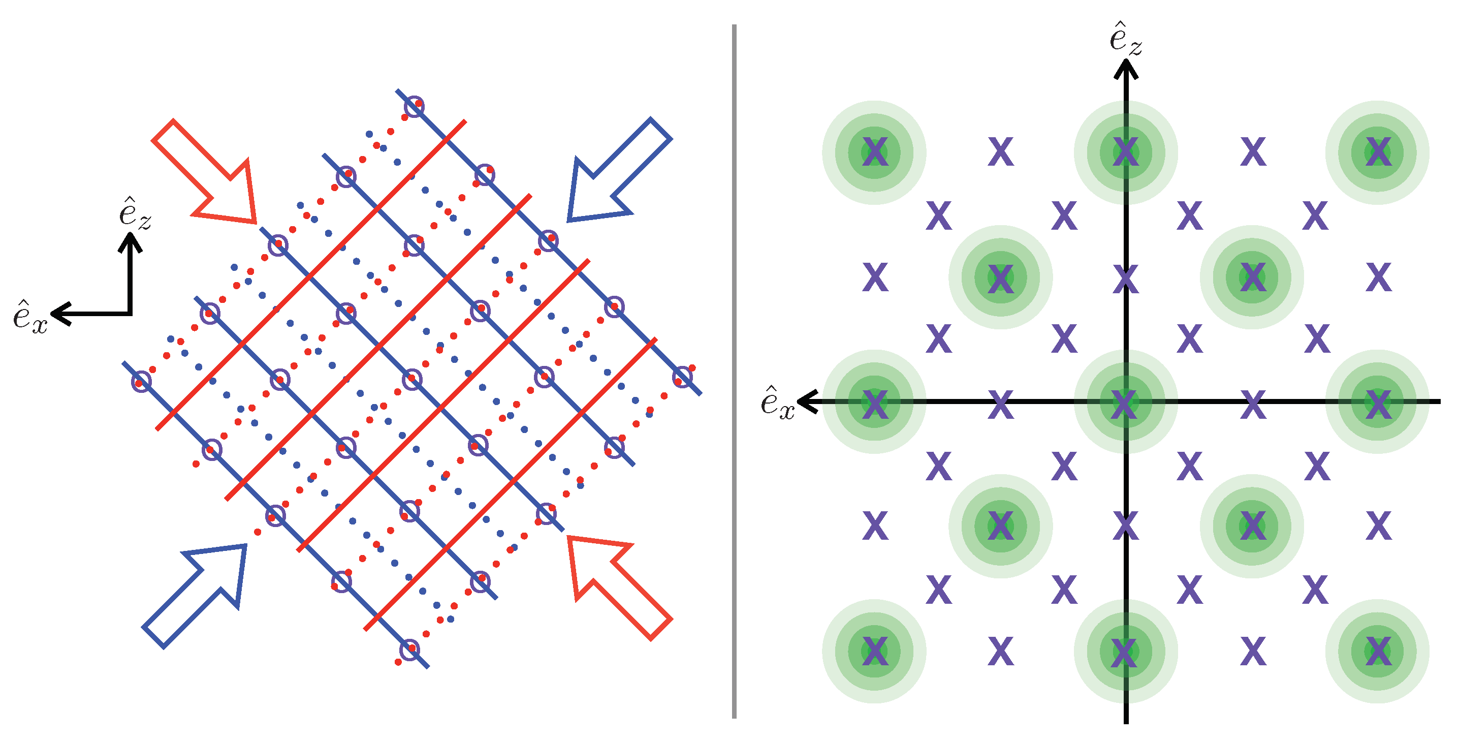
2.1. Light Field Geometry

Our experimental approach is an adaptation to a large sample of neutral atoms of the scheme originally developed by Fortson [18] for a single trapped ion. In the latter case, the ion is held in a tight secular orbit, relative to the wavelength of an applied light field. The light is two crossed standing waves, one of them having an intensity maximum in the trapping volume and the other having a node at the same location, as shown in Figure 1.

The two fields should both be resonant with an electric dipole forbidden transition. In both the seminal paper by Fortson and in our adaptation to an optical lattice configuration, the transition in question is from a 6s ground state to one of the fine-structure levels of the 5d state. In our case, this is in neutral Cs and in [18] it refers to the isoelectronic Ba⁺. The field having a node will address an E2 resonance and since the latter scales with the gradient of the field amplitude, it being driven at a field node maximises the induced E2 light shift.

The orthogonal field, with an anti-node overlapping the trapping volume, excites a weak E1 light shift induced by the parity violating mixing of both the 6s and 5d levels with a progression of p and f levels. The corresponding matrix element is of the following form:

$$A_{\mathrm{PNC}}({\psi }_{6\mathrm{s}}\leftrightarrow {\psi }_{5\mathrm{d}})\propto \sum _k\frac{\langle {\psi }_{5\mathrm{d}}|H_{\mathrm{E}1}|{\psi }_k\rangle \langle {\psi }_k|H_{\mathrm{PNC}}|{\psi }_{6\mathrm{s}}\rangle }{E_{6\mathrm{s}}-E_k}+\sum _k\frac{\langle {\psi }_{5\mathrm{d}}|H_{\mathrm{PNC}}|{\psi }_k\rangle \langle {\psi }_k|H_{\mathrm{E}1}|{\psi }_{6\mathrm{s}}\rangle }{E_{5\mathrm{d}}-E_k}.$$

(1)

The sums are taken over all states with opposite parity to 6s and 5d.

Provided that the interaction volume (in [18] corresponding to the localisation of the trapped ion) is small compared to the resonant wavelength, the ion experiences the two approximately homogeneous Rabi frequencies [19]:

$$\begin{array}{cc}\hfill {\mathsf{\Omega }}_{\mathrm{E}2}& =-\frac{1}{2\hslash }\sum _{i,j}{\left(A_{\mathrm{E}2}\right)}_{i,j}{\left[\frac{\partial {\mathcal{E}}_i\left(\mathbf{r}\right)}{\partial x_j}\right]}_{\mathbf{r}=\mathbf{0}}\hfill \\ \hfill \mathrm{and}{\mathsf{\Omega }}_{\mathrm{PNC}}& =-\frac{1}{2\hslash }\sum _i{\left(A_{\mathrm{PNC}}\right)}_i{\mathcal{E}}_i(\mathbf{r}=\mathbf{0}),\hfill \end{array}$$

(2)

where the indices represent the Cartesian coordinates and the tensor elements ${\left(A_{\mathrm{E}2}\right)}_{i,j}$ and ${\left(A_{\mathrm{PNC}}\right)}_i$ are the E2 and PNC amplitudes respectively.

The two interactions in Equation (2) combine to a total light shift given by:

$$\begin{array}{cc}\hfill \mathsf{\Delta }E& =\hslash \sqrt{|{\mathsf{\Omega }}_{\mathrm{E}2}+{\mathsf{\Omega }}_{\mathrm{PNC}}{|}^2}\hfill \\ \hfill & \approx \hslash {\mathsf{\Omega }}_{\mathrm{E}2}+\frac{\hslash \mathrm{Re}\left[{\mathsf{\Omega }}_{\mathrm{E}2}{\mathsf{\Omega }}_{\mathrm{PNC}}^{*}\right]}{{\mathsf{\Omega }}_{\mathrm{E}2}}\equiv W_{\mathrm{E}2}+W_{\mathrm{PNC}}.\hfill \end{array}$$

(3)

In the second line, the independent contribution of ${\mathsf{\Omega }}_{\mathrm{PNC}}$ has been ignored. It is too small to be in reach of experimental detection. However, the interference term, which we have labelled $W_{\mathrm{PNC}}$ can be accessible for measurements, provided that all systematic effects may be controlled ans discriminated against.

Applying the Fortson Scheme to a Large Sample on Neutral Atoms

While the scheme with a single ion benefits from the long integration time possible in an ion trap, the sample size of one is a problem. The scheme introduced in [17] confronts this problem by suggesting to trap a large sample of neutral atoms in a two-dimensional optical lattice. The crux with this is that every single atom must then be trapped, and well localised, around a point which fulfils the characteristics illustrated in Figure 1.

To accomplish this, the two crossed standing waves driving E2 and PNC amplitudes can still be applied in the same way. This will necessarily lead to a two-dimensional detection lattice, consisting of points where an optimised detection of the Fortson type is favoured. The experimental problem that leaves behind is then to devise a scheme that assures that every atom in a sample is well localised around a good detection point in the same 2D-plane.

This calls for a 2D optical lattice, and there is more than one way to design an optical lattice to fulfil the criterion in the previous paragraph. When doing this optical engineering, the element and the energy level structure in question must be considered. Additionally crucial is the interplay of beam geometry and polarisations, not only of the optical lattice beams but also of the E2 and PNC fields. This will determine spectroscopic selection rules.

The scheme we suggest is specifically designed for caesium and a detection of NSI light shift on the spectral line $6\mathrm{s}{}^2{\mathrm{S}}_{1/2}$–$5\mathrm{d}{}^2{\mathrm{D}}_{3/2}$—see Figure 2.

The proposed optical beam geometry is illustrated in Figure 3.

The E2 and PNC laser beams are resonant with the selected spectral line at ${\lambda }_{\mathrm{s}\mathrm{d}}=689.5$ nm, and both these cavity-enhanced standing waves are aligned in the $xz$-plane at angles of $\pi /4$ relative to the quantisation axis ${\widehat{\mathrm{e}}}_z$. The four optical lattices are along the ${\widehat{\mathrm{e}}}_x$ and ${\widehat{\mathrm{e}}}_z$-axes, polarised along ${\widehat{\mathrm{e}}}_y$ and tuned to a frequency exactly equal to the square root of two below the sd-resonance, ${\lambda }_{\mathrm{ol}}={\lambda }_{\mathrm{sd}}\sqrt{2}=975.1$ nm.

The electric fields of all laser beams are described by the equations:

$$\begin{array}{cc}\hfill {\mathcal{E}}_{\mathrm{ol}}(\mathbf{r},t)& =\frac{{\mathcal{E}}_{\mathrm{ol}}}{2}{\widehat{\mathrm{e}}}_y\{exp\left[-\mathrm{i}{k}_{\mathrm{ol}}{\widehat{\mathrm{e}}}_x·\mathbf{r}\right]+exp\left[\mathrm{i}{k}_{\mathrm{ol}}{\widehat{\mathrm{e}}}_x·\mathbf{r}\right]+exp\left[-\mathrm{i}{k}_{\mathrm{ol}}{\widehat{\mathrm{e}}}_z·\mathbf{r}\right]\hfill \\ \hfill & +exp\left[\mathrm{i}{k}_{\mathrm{ol}}{\widehat{\mathrm{e}}}_z·\mathbf{r}\right]\}{\mathrm{e}}^{\mathrm{i}{\omega }_{\mathrm{ol}}t}+\mathrm{c}.\mathrm{c}.\hfill \end{array}$$

(4)

$$\begin{array}{cc}\hfill {\mathcal{E}}_{\mathrm{E}2}(\mathbf{r},t)& =\frac{{\mathcal{E}}_{\mathrm{E}2}}{2\sqrt{2}}({\widehat{\mathrm{e}}}_x-{\widehat{\mathrm{e}}}_z)\{exp\left[-\frac{\mathrm{i}{k}_{\mathrm{sd}}}{\sqrt{2}}({\widehat{\mathrm{e}}}_x+{\widehat{\mathrm{e}}}_z)·\mathbf{r}\right]+exp\left[\frac{\mathrm{i}{k}_{\mathrm{sd}}}{\sqrt{2}}\left({\widehat{\mathrm{e}}}_x+{\widehat{\mathrm{e}}}_z\right)·\mathbf{r}+\mathrm{i}\pi \right]\}{\mathrm{e}}^{\mathrm{i}{\omega }_{\mathrm{sd}}t}+\mathrm{c}.\mathrm{c}.\hfill \end{array}$$

(5)

$$\begin{array}{cc}\hfill {\mathcal{E}}_{\mathrm{PNC}}(\mathbf{r},t)& =\frac{{\mathcal{E}}_{\mathrm{PNC}}}{2\sqrt{2}}({\widehat{\mathrm{e}}}_x+{\widehat{\mathrm{e}}}_z)\{exp\left[-\frac{\mathrm{i}{k}_{\mathrm{sd}}}{\sqrt{2}}({\widehat{\mathrm{e}}}_x-{\widehat{\mathrm{e}}}_z)·\mathbf{r}\right]+exp\left[\frac{\mathrm{i}k}{\sqrt{2}}({\widehat{\mathrm{e}}}_x-{\widehat{\mathrm{e}}}_z)·\mathbf{r}\right]\}{\mathrm{e}}^{\mathrm{i}{\omega }_{\mathrm{sd}}t}+\mathrm{c}.\mathrm{c}..\hfill \end{array}$$

(6)

The three factors $\mathcal{E}$, with the respective subscripts, are the amplitudes of the electric fields for the optical lattice, the E2 and PNC excitations. The $\omega$’s are angular frequencies and the $k=\omega /c$ the angular wave numbers. The relative phase of $\pi$ in ${\mathcal{E}}_{\mathrm{E}2}$ ensures that a nodal plane crosses the origin. For all beams, the temporal phases have to be interferometrically controlled. Since all laser beams appear in counter-propagating pairs, there is no need to lock the relative phase between the two lasers at ${\lambda }_{\mathrm{sd}}$ and ${\lambda }_{\mathrm{ol}}$. Any global phase drift in any of them will appear equally in all arms, meaning that all phase drifts before the respective beams are split will cancel (see [20] or [21]).

As in Figure 1, the setup generated by Equations (5) and (6) gives us two orthogonal standing waves, one driving an E2-transition and the other one inducing a PNC light shift. The difference is that, instead of limiting the field of view to one point in space, we look at the entire plane spanned by the two beams. This will have a periodic pattern of points fulfilling the detection requirements (E2 nodal point overlapping a PNC anti-nodal point).

In order to ensure a uniform irradiance in the interaction region, the E2 and PNC beams should have a near-flat distribution, using techniques such as, for example, in [22] or [23]. This should give an interaction region of approximately the cube of the E2 and PNC beam diameters. In addition, to remove atoms lingering outside the detection volume, clean-up beams resonant at the D1 and D2 lines should be focused to the regions directly outside the volume, directly before the spectroscopic measurement. Also for the optical lattice, it is beneficial with an irradiance distribution in the interaction region as homogeneous as possible.

The optical lattice will ensure that every atom in the sample is tightly confined in the 2D-plane around a valid detection point. The configuration in Equation (4) yields a square optical lattice with the light shift potential [24,25,26]:

$$U\left(\mathbf{r}\right)=U_0\left[{cos}^2\left(k_{\mathrm{ol}}x\right)+{cos}^2\left(k_{\mathrm{ol}}z\right)+2cos\left(k_{\mathrm{ol}}x\right)cos\left(k_{\mathrm{ol}}z\right)\right],$$

(7)

where $U_0$ is the light shift at irradiance maxima. In Figure 4, we show an illustration of the overlapping grids of trapping and detection sites. There will be detection point that do not have an atom, but this is of no consequence.

The experimental sequence will be initiated by atoms being accumulated in a magneto-optical trap (MOT). The thermal motion will then be reduced by three-dimensional laser cooling to temperatures of the order of 1 $\mathsf{\mu }$K. The final preparatory step is then to adiabatically transfer them to the optical lattice in Equation (4).

For all involved laser beams, it will be critical to have sufficient power. The final PNC signature will scale as the square root of the irradiance—see Equation (2). For the optical lattice, higher irradiance means tighter confinement. Ideally, the atoms should be trapped in the Lamb–Dicke regime. This keeps them confined in an area in the 2D-plane small compared to ${\lambda }_{\mathrm{s}\mathrm{d}}^2$.

Intense lasers, for all beams, also facilitates uniform Rabi frequencies and potential depths. In Section 4, we provide a case study where we, as an example, assume lasers close to the limit to what is currently commercially available.

2.2. Spectroscopic Detection Scheme

In order to achieve an unambiguous experimental signature of PNC, two main hurdles have to be overcome:

• The detection scheme must isolate the parity-violating component of the total signal.
• A plethora of systematic effects have to be confronted.

To this effect, we suggest employing a spectroscopic scheme inspired by [27]. The core idea is to measure several splittings in the ground-state manifold of Zeeman sublevels, with opposite signs of the angular momentum projection $M_F$. This will all but eliminate the main systematics effects, namely the E1 light shift induced by the trapping potential, the linear Zeeman shift and the pure E2 light shift contribution in Equation (2). The only linear effect that will not be eliminated, when comparing the mirrored spectral signals, is the parity-violating contribution. In this particular scheme that we present, an NSI PNC signature is isolated, and we have selected the resolved hyperfine structure (hfs) transition $F=4\leftrightarrow F^{\prime }=5$ on the line $6\mathrm{s}{}^2{\mathrm{S}}_{1/2}$–$5\mathrm{d}{}^2{\mathrm{D}}_{3/2}$. This leaves us with nine Zeeman states ($M_F$) in the ground state, see Figure 5. We assume that the sample has been initially optically pumped, in order to leave the majority of the population in $6\mathrm{s}{}^2{\mathrm{S}}_{1/2},F=4$.

To pinpoint NSI we need the E2 and PNC fields to drive $\mathsf{\Delta }{M}_F=0$ transitions. The polarisations and the beam propagation directions in Equations (5) and (6), and in Figure 3, have been chosen with this in mind. The PNC beam polarisation will drive $\pi$-transitions. For the E2 field, $\mathsf{\Delta }{M}_F=0$ will be strongly favoured, and $\mathsf{\Delta }{M}_F=\pm 1$ will be completely suppressed (see [19]). The lingering small $\mathsf{\Delta }{M}_F=\pm 2$ transition probability will be eliminated by adding a bias field of minimum 3 mT along ${\widehat{\mathrm{e}}}_z$. That will shift spin-changing transitions sufficiently out of resonance. This field will also serve the purpose of fixing the quantisation axis.

The total $M_F$ dependent light shift in the $6\mathrm{s}{}^2{\mathrm{S}}_{1/2}$ ground state of an atom trapped in the optical lattice, and interacting with the detection field, is:

$$\mathsf{\Delta }E\left(M_F\right)=M_F{E}_{\mathrm{Z}}+E_{\mathrm{qZ},M}+U_{0,M}+W_{\mathrm{E}2,\mathrm{M}}+W_{\mathrm{PNC},\mathrm{M}}.$$

(8)

The two last terms are the light shifts from Equation (3) and we have assumed that the the corresponding light is exactly on the resonance ${\lambda }_{\mathrm{s}\mathrm{d}}$. $U_{0,M}$ is the E1 light shift at the centre of the trapping volume, induced by the optical lattice. We assume that the atoms are sufficiently tightly confined to consider this as uniform. $E_{\mathrm{Z}}$ and $E_{\mathrm{qZ},M}$ are Larmor frequencies in energy units due to, respectively, the linear and quadratic Zeeman effect. With ‘quadratic Zeeman effect’ we here refer to the quadratic term arising in the intermediate region between the weak Zeeman effect and the Paschen–Back effect (see e.g., [28]).

The series of levels shift in both ground and excited states as illustrated in Figure 5. The shifts for the ground state levels are:

$$\begin{array}{cc}\hfill \mathsf{\Delta }E(+4)& =4E_{\mathrm{Z}}+U_{0,4}+W_{\mathrm{E}2,3}+W_{\mathrm{PNC},4}\hfill \\ \hfill \mathsf{\Delta }E(+3)& =3E_{\mathrm{Z}}+E_{\mathrm{qZ},3}+U_{0,3}+W_{\mathrm{E}2,3}+W_{\mathrm{PNC},3}\hfill \\ \hfill \mathsf{\Delta }E(+2)& =2E_{\mathrm{Z}}+E_{\mathrm{qZ},2}+U_{0,2}+W_{\mathrm{E}2,2}+W_{\mathrm{PNC},2}\hfill \\ \hfill \mathsf{\Delta }E(+1)& =E_{\mathrm{Z}}+E_{\mathrm{qZ},1}+U_{0,1}+W_{\mathrm{E}2,1}+W_{\mathrm{PNC},1}\hfill \\ \hfill \mathsf{\Delta }E\left(0\right)& =E_{\mathrm{qZ},0}+U_{0,0}+W_{\mathrm{E}2,0}+W_{\mathrm{PNC},0}\hfill \\ \hfill \mathsf{\Delta }E(-1)& =-E_{\mathrm{Z}}+E_{\mathrm{qZ},-1}+U_{0,1}+W_{\mathrm{E}2,1}-W_{\mathrm{PNC},1}\hfill \\ \hfill \mathsf{\Delta }E(-2)& =-2E_{\mathrm{Z}}+E_{\mathrm{qZ},-2}+U_{0,2}+W_{\mathrm{E}2,2}-W_{\mathrm{PNC},2}\hfill \\ \hfill \mathsf{\Delta }E(-3)& =-3E_{\mathrm{Z}}+E_{\mathrm{qZ},-3}+U_{0,3}+W_{\mathrm{E}2,3}-W_{\mathrm{PNC},3}\hfill \\ \hfill \mathsf{\Delta }E(-4)& =-4E_{\mathrm{Z}}+U_{0,4}+W_{\mathrm{E}2,3}-W_{\mathrm{PNC},4}.\hfill \end{array}$$

(9)

It should be noted that the E2 light shifts are the same for the states $M_F=\pm 3$ as for $M_F=\pm 4$. The $\mathsf{\Delta }{M}_F=0$ transitions for these states have the same Clebsch–Gordan coefficients.

The relative energies of the manifold of Zeeman states should now be accurately measured. The PNC shift will bring about a subtle break in the symmetry apparent in Figure 5, and with a careful choice of measurements of splittings, this could be uncovered form the other effects. A schematic illustration of our proposed scheme is included in the lower part of Figure 5.

2.2.1. RF and Raman Spectroscopy

The specific Zeeman splittings that we pinpoint are $M_F=-4\leftrightarrow M_F=-3$, $M_F=-1\leftrightarrow M_F=1$ and $M_F=3\leftrightarrow M_F=4$ (see Figure 5). The two at the stretched ends of the manifold will be addressed with radio-frequency (RF) spectroscopy (see [19] for details). Specifically, this should be done by Ramsey spectroscopy with a combination of a microwave radiation at 9.2 GHz (the ground state hfs splitting) and induced fluorescence. The suitable measurement duration is the lifetime of the 5d level (approximately one microsecond [29]). This will yield two spectra, respectively centred on the energies:

$$\begin{array}{cc}\hfill \hslash {\omega }_{\mathrm{RF},\mathrm{a}}& =\mathsf{\Delta }E(+4)-\mathsf{\Delta }E(+3)\hfill \\ \hfill \mathrm{and}\hslash {\omega }_{\mathrm{RF},\mathrm{b}}& =\mathsf{\Delta }E(-4)-\mathsf{\Delta }E(-3),\hfill \end{array}$$

(10)

The remaining Zeeman state energy difference needed is $M_F=-1\leftrightarrow M_F=1$. It is not easily accessible by RF spectroscopy. Instead, with two laser beams of equal irradiance and a small and tunable relative detuning, a spectrum is acquired by stimulated Raman spectroscopy. The balancing of the intensities eliminates additional light shifts caused by the Raman beams. The central energy will be:

$$\hslash {\omega }_{\mathrm{Raman}}=\mathsf{\Delta }E(+1)-\mathsf{\Delta }E(-1).$$

(11)

The cancellation of systematic effects is a crucial feature of the scheme. To optimise this, the spectroscopies should be made all at once, following ideas developed by the atomic clock community, see [30].

2.2.2. Isolation of the PNC Signature

The central angular frequencies in Equations (10) and (11) should be combined as:

$$\begin{array}{cc}\hfill \hslash & \left({\omega }_{\mathrm{RF},\mathrm{a}}-{\omega }_{\mathrm{RF},\mathrm{b}}-{\omega }_{\mathrm{Raman}}\right)\hfill \\ \hfill & =\left(W_{\mathrm{PNC},4}-W_{\mathrm{PNC},3}-W_{\mathrm{PNC},1}\right)+E_{\mathrm{qZ}}\hfill \\ \hfill & =\hslash {\omega }_{\mathrm{obs}}+E_{\mathrm{qZ}}.\hfill \end{array}$$

(12)

The subtraction of signals in Equation (12) leaves us with one spectral signature which is the PNC signature that we will eventually want to isolate. Remaining in Equation (12) is the quadratic part of the Zeeman shift, which is insensitive to mirroring spectroscopy. The latter shift will remain a considerable systematic effect. It will have to be controlled by minimising ambient fields and by a spectroscopic in situ determination of the remnant shift. Techniques for how to further minimise this error contribution are explained in [31].

In Section 4, we will combine the expression in Equations (9) and (12) with theoretical computations of the relevant transition matrix elements (see Section 3) in order to estimate an expected final result.

3. Theoretical Methods

To calculate transition matrix elements, we consider an atomic Hamiltonian ($H_{\mathrm{at}}$) emerging from the Dirac–Coulomb interactions. Thereby, we account for the relativistic and electron correlation effects in the calculations of atomic wave functions. In atomic units (a.u.), this is given by:

$$H_{\mathrm{at}}=\sum _i\left[c{\mathit{\alpha }}_i·{\mathbf{p}}_i+({\beta }_i-1)c^2+V_{\mathrm{n}}\left(r_i\right)+\sum _{j>i}{V}_{\mathrm{C}}\left(r_{ij}\right)\right],$$

(13)

with $\mathit{\alpha }$ and $\beta$ being the Dirac matrices (see e.g., [1]). $V_{\mathrm{n}}\left(r\right)$ represents the nuclear potential and $V_{\mathrm{C}}\left(r_{ij}\right)=\frac{1}{r_{ij}}$ is the Coulomb interaction potential for one electron pair. To evaluate the nuclear charge density ${\rho }_{\mathrm{n}}\left(r\right)$ and $V_{\mathrm{n}}\left(r\right)$, we consider the Fermi-charge distribution defined by [32]:

$${\rho }_{\mathrm{n}}\left(r_i\right)=\frac{{\rho }_0}{1+{\mathrm{e}}^{(r_i-b)/a}}.$$

(14)

Here, ${\rho }_0$ is a normalisation factor, and the half-charge radii b and $a=2.3/4(ln3)$ are related to the skin thickness. We have used the value $b=5.670729105$ fm [33] in our calculations.

The ground state electronic configuration of neutral Cs is $\left[5{\mathrm{p}}^6\right]6\mathrm{s}$ (see Figure 2). The configurations of low-lying excited states differ only with respect to the valence $6\mathrm{s}$ orbital being replaced by another one. Atomic wave functions of these states can be conveniently determined by considering the closed-shell electronic configuration first, and then appending the respective valence orbital. We consider the Dirac–Hartree–Fock (DHF) method as a path to obtain the mean-field wave function ($|{\mathsf{\Phi }}_0\rangle$) of the $\left[5{\mathrm{p}}^6\right]$ configuration. The DHF wave function of the relevant atomic states of Cs atoms are then defined by $|{\varphi }_v\rangle =a_v^{†}|{\mathsf{\Phi }}_0\rangle$ with $a_v^{†}$ representing the respective appended valence orbital v.

The single particle orbitals of this DHF wave function are defined as [34]:

$${\phi }_{n,\kappa ,m}(r,\theta ,\varphi )=\frac{1}{r}\left(\begin{array}{cc}{P}_{n,\kappa }\left(r\right)& {\chi }_{\kappa ,m}(\theta ,\varphi )\\ \mathrm{i}{Q}_{n,\kappa }\left(r\right)& {\chi }_{-\kappa ,m}(\theta ,\varphi )\end{array}\right),$$

(15)

where $P_{n,\kappa }\left(r\right)$ and $Q_{n,\kappa }\left(r\right)$ are the large and small component radial functions, while ${\chi }_{\kappa ,m}(\theta ,\varphi )$ and ${\chi }_{-\kappa ,m}(\theta ,\varphi )$ are the respective four component spinors for the principal quantum number n and the relativistic angular momentum quantum number $\kappa$. The radial components are constructed using Gaussian type orbitals (GTOs) [35]. That is:

$$P_{n,\kappa }\left(r\right)=\sum _{k=1}^{N_k}{C}_{\kappa ,k}^L{g}_{\kappa ,k}^L\left(r\right)$$

(16)

and

$$Q_{n,\kappa }\left(r\right)=\sum _{k=1}^{N_k}{C}_{\kappa ,k}^S{g}_{\kappa ,k}^S\left(r\right),$$

(17)

where k sums over the total number of GTOs ($N_k$) in each symmetry, $C_{\kappa ,k}^{L/S}$ are the unknown coefficients that need to be determined and $g_{\kappa ,k}^{L/S}$ are the GTOs for the large (L) and small (S) components, respectively.

The GTOs for the large radial component are defined as:

$$g_{\kappa ,k}^L\left(r\right)={\mathcal{N}}_{\kappa ,k}^L{r}^{l+1}{\mathrm{e}}^{-\left({\eta }_k{r}^2\right)},$$

(18)

where ${\mathcal{N}}_{\kappa ,k}^L$ represents a normalisation constant, ${\eta }_k$ is an arbitrary coefficient suitably chosen for accurate calculations of wave functions and l is the orbital quantum number of the orbital. The exponents ${\eta }_k$ form an even-tempered series,

$${\eta }_k={\eta }_0{\zeta }^{k-1},$$

(19)

in terms of the parameters ${\eta }_0$ and $\zeta$.

However, GTOs for the small radial component are defined by implementing a kinetic balance condition as

$$g_{\kappa ,k}^S\left(r\right)={\mathcal{N}}_{\kappa ,k}^S\left(\frac{\mathrm{d}}{\mathrm{d}r}+\frac{\kappa }{r}\right)g_{\kappa ,k}^L\left(r\right),$$

(20)

with the corresponding normalisation constant ${\mathcal{N}}_{\kappa ,k}^S$. In

Table 1. Lists of ${\eta }_0$, $\zeta$ and number of Gaussian type orbitals (GTOs) ($N_k$) used to define the basis functions for different symmetries in the construction of single particle orbitals in the present calculations. In the bottom row, we also give the number of active orbitals ($N_v$) allowed to participate in the estimation of electron correlation effects, using the RCCSD method.

	$\mathbf{s}$	$\mathbf{p}$	$\mathbf{d}$	$\mathbf{f}$	$\mathbf{g}$	$\mathbf{h}$	$\mathbf{i}$
${\eta }_0$	$0.00009$	$0.0008$	$0.001$	$0.004$	$0.005$	$0.005$	$0.005$
$\zeta$	2.15	2.15	2.15	2.25	2.35	2.35	2.35
$N_k$	40	39	38	37	36	35	33
$Nv$	1–19	2–19	3–19	4–17	5–15	6–13	7–13

, we give the list of ${\eta }_0$ and $\zeta$ parameters, along with $N_k$ for each symmetry used in the present calculations.

The interaction Hamiltonian due to the NSI PNC interaction is given by [36]:

$$H_{\mathrm{PNC}}^{\mathrm{NSI}}=-\frac{G_{\mathrm{F}}}{2\sqrt{2}}{Q}_W{\gamma }_5{\rho }_n\left(r\right)\equiv \lambda H_{\mathrm{weak}},$$

(21)

where $G_{\mathrm{F}}$ is the Fermi constant and ${\gamma }_5$ is the product of the four Dirac matrices. In the above expression, we have defined $H_{\mathrm{weak}}$ by considering $\lambda =\frac{G_F}{2\sqrt{2}}{Q}_W$. Owing to the odd parity of the $H_{\mathrm{weak}}$ interaction, the $A_{\mathrm{PNC}}$ amplitude between the same nominal parity $|{\mathsf{\Psi }}_{\mathrm{i}}\rangle$ and $|{\mathsf{\Psi }}_{\mathrm{f}}\rangle$ states is given by:

$$A_{\mathrm{PNC}}=\frac{\langle {\mathsf{\Psi }}_{\mathrm{f}}|H_{\mathrm{E}1}|{\mathsf{\Psi }}_{\mathrm{i}}\rangle }{\sqrt{\langle {\mathsf{\Psi }}_{\mathrm{f}}|{\mathsf{\Psi }}_{\mathrm{f}}\rangle \langle {\mathsf{\Psi }}_{\mathrm{i}}|{\mathsf{\Psi }}_{\mathrm{i}}\rangle }}.$$

(22)

Since $H_{\mathrm{PNC}}^{\mathrm{NSI}}$ is very weak with respect to the main structural Hamiltonian, $H_{\mathrm{at}}$, the eigenfunction ($|{\mathsf{\Psi }}_v\rangle$) to the total Hamiltonian $H=H_{\mathrm{at}}+\lambda H_{\mathrm{weak}}$, and its energy ($E_v$), can be expressed as:

$$\begin{array}{cc}\hfill & |{\mathsf{\Psi }}_v\rangle =|{\mathsf{\Psi }}_v^{\left(0\right)}\rangle +\lambda |{\mathsf{\Psi }}_v^{\left(1\right)}\rangle +\mathcal{O}\left({\lambda }^2\right)\hfill \\ \hfill \mathrm{and}& \hfill \\ \hfill & E_v=E_v^{\left(0\right)}+\lambda |{\mathsf{\Psi }}_v^{\left(1\right)}\rangle +\mathcal{O}\left({\lambda }^2\right),\hfill \end{array}$$

(23)

where the superscripts 0 and 1 represent the zeroth-order and first-order perturbation contributions due to $H_{\mathrm{weak}}$. By neglecting $\mathcal{O}\left({\lambda }^2\right)$ contributions, we get:

$$A_{\mathrm{PNC}}\simeq \frac{\langle {\mathsf{\Psi }}_{\mathrm{f}}^{\left(1\right)}|H_{\mathrm{E}1}|{\mathsf{\Psi }}_{\mathrm{i}}^{\left(0\right)}\rangle +\langle {\mathsf{\Psi }}_{\mathrm{f}}^{\left(0\right)}|H_{\mathrm{E}1}|{\mathsf{\Psi }}_{\mathrm{i}}^{\left(1\right)}\rangle }{\sqrt{\langle {\mathsf{\Psi }}_{\mathrm{f}}^{\left(0\right)}|{\mathsf{\Psi }}_{\mathrm{f}}^{\left(0\right)}\rangle \langle {\mathsf{\Psi }}_{\mathrm{i}}^{\left(0\right)}|{\mathsf{\Psi }}_{\mathrm{i}}^{\left(0\right)}\rangle }}.$$

(24)

In the sum-over-states approach, the first-order wave function is then written as

$$|{\mathsf{\Psi }}_n^{\left(1\right)}\rangle =\sum _{I\ne n}|{\mathsf{\Psi }}_I^{\left(0\right)}\rangle \frac{\langle {\mathsf{\Psi }}_I^{\left(0\right)}|H_{\mathrm{weak}}|{\mathsf{\Psi }}_n^{\left(0\right)}\rangle }{E_n^{\left(0\right)}-E_I^{\left(0\right)}}.$$

(25)

The limitation of this approach is that, in an actual calculation, it is only possible to include contributions from a few low-lying valence excited bound states, by calculating them individually using a suitable many-body method. However, to achieve high accuracy for $A_{\mathrm{PNC}}$ calculations, it is often necessary to include contributions from the core and continuum states. Again, core-polarization effects simultaneously due to the PNC interaction Hamiltonian and the dipole operator cannot be included in a sum-over-states approach.

The above problems are circumvented by obtaining the first-order perturbed wave functions for the initial and final states directly. From the equation $H|{\mathsf{\Psi }}_v\rangle =E_v|{\mathsf{\Psi }}_v\rangle$, the first-order wave function satisfies:

$$(H_{\mathrm{at}}-E_v^{\left(0\right)})|{\mathsf{\Psi }}_v^{\left(1\right)}\rangle =(E_v^{\left(1\right)}-H_{\mathrm{weak}})|{\mathsf{\Psi }}_v^{\left(0\right)}\rangle .$$

(26)

To account for the electron correlation effects to all-orders, we apply relativistic coupled-cluster (RCC) theory, in which the exact wave function of the $\left[5{\mathrm{p}}^6\right]$ configuration is expressed as [37,38]:

$$|{\mathsf{\Psi }}_0\rangle ={\mathrm{e}}^T|{\mathsf{\Phi }}_0\rangle ,$$

(27)

where T is the particle-hole excitation operator. For states described by the $\left[5{\mathrm{p}}^6\right]$ closed core configuration and the valence orbital (v), the atomic wave function can be expressed in the RCC theory as [39]:

$$\begin{array}{cc}\hfill |{\mathsf{\Psi }}_v\rangle & ={\mathrm{e}}^{T+S_v}|{\mathsf{\Phi }}_v\rangle \hfill \\ \hfill & ={\mathrm{e}}^T\left\{1+S_v\right\}|{\mathsf{\Phi }}_v\rangle ,\hfill \end{array}$$

(28)

where $S_v$ is another RCC operator, which excites the valence orbital to a virtual orbital and a valence-core pair to the unoccupied virtual orbitals.

To obtain the unperturbed and perturbed wave functions, we perturb the RCC operators as [40]:

$$T=T^{\left(0\right)}+\lambda T^{\left(1\right)}+\mathcal{O}\left({\lambda }^2\right)$$

(29)

and

$$S_v=S_v^{\left(0\right)}+\lambda S_v^{\left(1\right)}+\mathcal{O}\left({\lambda }^2\right),$$

(30)

where $T^{(0/1)}$ and $S_v^{(0/1)}$ are the core and the valence excitation operators, with the superscripts 0 and 1 representing the zeroth and first-order perturbations due to $H_{\mathrm{weak}}$. Substituting the above operators in the earlier expressions, and equating the zeroth- and first-order in orders of $\lambda$ terms, yields:

$$\begin{array}{cc}\hfill |{\mathsf{\Psi }}_v^{\left(0\right)}\rangle & ={\mathrm{e}}^{T^{\left(0\right)}}\left\{1+S_v^{\left(0\right)}\right\}|{\mathsf{\Phi }}_v\rangle \hfill \\ \hfill \mathrm{and}|{\mathsf{\Psi }}_v^{\left(1\right)}\rangle & ={\mathrm{e}}^{T^{\left(0\right)}}\left\{S_v^{\left(1\right)}+T^{\left(1\right)}\left(1+S_v^{\left(0\right)}\right)\right\}|{\mathsf{\Phi }}_v\rangle .\hfill \end{array}$$

(31)

The amplitudes of the unperturbed RCC operators and energies are obtained by solving the following equations (see e.g., [40,41]):

$$\langle {\mathsf{\Phi }}_K|{\overline{H}}_{\mathrm{at}}|{\mathsf{\Phi }}_0\rangle ={\delta }_{K,0}{E}_0^{\left(0\right)}$$

(32)

and

$$\langle {\mathsf{\Phi }}_L|{\overline{H}}_{\mathrm{at}}\{1+S_v^{\left(0\right)}\}|{\mathsf{\Phi }}_v\rangle =E_v^{\left(0\right)}\langle {\mathsf{\Phi }}_L|\{{\delta }_{L,v}+S_v\}|{\mathsf{\Phi }}_v\rangle ,$$

(33)

with ${\overline{H}}_{\mathrm{at}}={\mathrm{e}}^{-T^{\left(0\right)}}{H}_{\mathrm{at}}{\mathrm{e}}^{T^{\left(0\right)}}$. The superscripts K and L indicate the $K^{\mathrm{th}}$ and $L^{\mathrm{th}}$ excited determinants with respect to $|{\mathsf{\Phi }}_0\rangle$ and $|{\mathsf{\Phi }}_v\rangle$.

The energies are evaluated as

$$E_0^{\left(0\right)}=\langle {\mathsf{\Phi }}_0|{\overline{H}}_{\mathrm{at}}|{\mathsf{\Phi }}_0\rangle$$

(34)

and

$$E_v^{\left(0\right)}=\langle {\mathsf{\Phi }}_v|{\overline{H}}_{\mathrm{at}}\left\{1+S_v^{\left(0\right)}\right\}|{\mathsf{\Phi }}_n\rangle .$$

(35)

It follows that the difference between $E_v^{\left(0\right)}$ and $E_0^{\left(0\right)}$ yields the binding energy of an electron in the valence orbital v. Similarly, amplitudes of the perturbed RCC operators are obtained by:

$$\langle {\mathsf{\Phi }}_K|{\overline{H}}_{\mathrm{at}}{T}^{\left(1\right)}+{\overline{H}}_{\mathrm{weak}}|{\mathsf{\Phi }}_0\rangle =0$$

(36)

and

$$\langle {\mathsf{\Phi }}_L|({\overline{H}}_{\mathrm{at}}-E_v^{\left(0\right)})S_v^{\left(1\right)}+({\overline{H}}_{\mathrm{at}}{T}^{\left(1\right)}+{\overline{H}}_{\mathrm{weak}})\times \{1+S_v^{\left(0\right)}\}|{\mathsf{\Phi }}_v\rangle =0,$$

(37)

where ${\overline{H}}_{\mathrm{weak}}={\mathrm{e}}^{-T^{\left(0\right)}}{H}_{\mathrm{weak}}{\mathrm{e}}^{T^{\left(0\right)}}$.

After obtaining amplitudes for the unperturbed and perturbed RCC operators, we evaluate the $\mathrm{E}{1}_{\mathrm{PNC}}$ amplitude as:

$$A_{\mathrm{PNC}}\simeq \frac{\langle {\mathsf{\Phi }}_{\mathrm{f}}|\{S_{\mathrm{f}}^{\left(1\right)}+(S_{\mathrm{f}}^{\left(0\right)†}+1)T^{\left(1\right)†}\}{\overline{H}}_{\mathrm{E}1}\{1+S_{\mathrm{i}}^{\left(0\right)}\}+\{S_{\mathrm{f}}^{\left(0\right)†}+1\}{\overline{H}}_{\mathrm{E}1}\{T^{\left(1\right)}(1+S_{\mathrm{i}}^{\left(0\right)})+S_{\mathrm{i}}^{\left(1\right)}\}|{\mathsf{\Phi }}_{\mathrm{i}}\rangle }{\langle {\mathsf{\Phi }}_{\mathrm{f}}|\{S_{\mathrm{f}}^{\left(0\right)†}+1\}\overline{N}\{1+S_{\mathrm{i}}^{\left(0\right)}\}|{\mathsf{\Phi }}_{\mathrm{i}}\rangle },$$

(38)

where ${\overline{H}}_{\mathrm{E}1}={\mathrm{e}}^{T^{\left(0\right)†}}{H}_{\mathrm{E}1}{\mathrm{e}}^{T^{\left(0\right)}}$ and $\overline{N}={\mathrm{e}}^{T^{\left(0\right)†}}{\mathrm{e}}^{T^{\left(0\right)}}$. The ‘Core’ contributions for the initial and final states originate from $T^{\left(1\right)†}{\overline{H}}_{\mathrm{E}1}$ and ${\overline{H}}_{\mathrm{E}1}{T}^{\left(1\right)}$, and the rest of the RCC terms involving $S_{\mathrm{f}}^{(0/1)†}$ and $S_{\mathrm{i}}^{(0/1)}$ give rise to valence contributions from the ‘final’ and ‘initial’ states, respectively.

We have also evaluated transition amplitudes due to the electric dipole ($A_{\mathrm{E}1}$), electric quadrupole ($A_{\mathrm{E}2}$) and magnetic dipole ($A_{\mathrm{M}1}$) electromagnetic channels by using the unperturbed wave functions in the expression:

$$\begin{array}{cc}\hfill {\langle O\rangle }_{\mathrm{fi}}& =\frac{\langle {\mathsf{\Psi }}_{\mathrm{f}}^{\left(0\right)}|O|{\mathsf{\Psi }}_{\mathrm{i}}^{\left(0\right)}\rangle }{\sqrt{\langle {\mathsf{\Psi }}_{\mathrm{f}}^{\left(0\right)}|{\mathsf{\Psi }}_{\mathrm{f}}^{\left(0\right)}\rangle \langle {\mathsf{\Psi }}_{\mathrm{i}}^{\left(0\right)}|{\mathsf{\Psi }}_{\mathrm{i}}^{\left(0\right)}\rangle }}\hfill \\ \hfill & =\frac{\langle {\mathsf{\Phi }}_{\mathrm{f}}|\{S_{\mathrm{f}}^{\left(0\right)†}+1\}\overline{O}\{1+S_{\mathrm{i}}^{\left(0\right)}\}|{\mathsf{\Phi }}_{\mathrm{i}}\rangle }{\langle {\mathsf{\Phi }}_{\mathrm{f}}|\{S_{\mathrm{f}}^{\left(0\right)†}+1\}\overline{N}\{1+S_{\mathrm{i}}^{\left(0\right)}\}|{\mathsf{\Phi }}_{\mathrm{i}}\rangle },\hfill \end{array}$$

(39)

where $\overline{O}={\mathrm{e}}^{T^{\left(0\right)†}}O{\mathrm{e}}^{T^{\left(0\right)}}$ for the respective transition operator O, and $\overline{N}={\mathrm{e}}^{T^{\left(0\right)†}}{\mathrm{e}}^{T^{\left(0\right)}}$. We have incorporated one-particle and one-hole (single) and two-particle and two-hole (double) excitations of the RCC theory (RCCSD method) to carry out all the calculations. The number of active orbitals ($N_v$) considered for each angular momentum symmetry in the RCCSD method are mentioned in Table 1.

4. Results

In this section, we will first report on the results of the theoretical calculation. In addition the eigenvalues of this data for ¹³³Cs, they are necessary for a prediction of the parity violation signature in Equation (12) and thus for a check of the experimental feasibility. The various calculated transition amplitudes will also be essential for a proper estimate of experimental error contributions.

The relevant quantities in the spectroscopic investigations are the different light shifts. To estimate these, computed matrix elements must be combined with relevant Clebsch–Gordan coefficients and amplitudes of the driving laser fields. For a successful measurement, the irradiance of both the laser driving the E2 and PNC transitions on the 6s-5d line (sd-laser) and the one generating the optical lattice (ol-lattice) will be highly critical. The final measured PNC signature scales as the square root of the sd-laser irradiance (see Equation (2)). The importance of the ol-laser intensity is related to the achievable localisation of the atoms around optimised detection sites, as in Figure 4, and for the homogeneity of the E1 light shift across the interaction volume.

As projected laser powers, we have assumed ones from sources being at the top end of what is currently possible to obtain from commercial suppliers. These numbers are possible to improve, at least slightly, in an laboratory environment, and they will certainly increase with the advancement of laser technology. In

Table 2. Hypothesised laser parameters for the sd- and ol-lasers. P is the total laser power, $Q_{\mathrm{ef}}$ a cavity enhancement factor, w the beam diameter at the interaction region, ${\mathcal{E}}_{\mathrm{int}}$ the field amplitude at the detection sites and the final column shows the maximum reduction in amplitude at the edge of the interaction region. To estimate the numbers for the sd-laser, we have used [22]. For the ol-laser, the amplitude refers to the total one, taking into account all lattice beams (see (7)).

	$\mathit{\lambda }$ (nm)	P (W)	${\mathit{Q}}_{\mathbf{ef}}$	w (mm)	Mode	${\mathcal{E}}_{\mathbf{int}}$(V/m)	$\mathsf{\Delta }{\mathcal{E}}_{\mathbf{max}}/{\mathcal{E}}_{\mathbf{int}}$
sd-laser	689.5	3	100	0.5	flat-top	≃$3\times {10}^6$	0.015
ol-laser	975.1	5	1	1.5	Gaussian	≃$1\times {10}^5$	0.03

, we show the assumed laser powers applied in derivations that will follow in this section together with the corresponding relevant field amplitude and other important parameters.

To derive the electric field amplitudes ${\mathcal{E}}_{\mathrm{E}2}={\mathcal{E}}_{\mathrm{PNC}}=3\times {10}^6$ V/m for the sd-laser, we have assumed that E2 and PNC standing waves are cavity-enhanced with a factor of 100. The parameters for the sd-laser are such that they give a similar field amplitude to that used by Fortson in [18].

4.1. Theoretical Results

The calculations described in Section 3 are essential for an analysis of the feasibility of the experimental method. When the actual experiment is done, these computed quantities will be crucial for an interpretation of the experimental data.

4.1.1. Calculated PNC, E2 and M1 Matrix Elements and Associated Light Shifts

The results for the transition amplitudes on the PNC-NSI, E2 and M1 amplitudes on the electric dipole forbidden $6\mathrm{s}{}^2{\mathrm{S}}_{1/2}$–$5\mathrm{d}{}^2{\mathrm{D}}_{1/2}$ transition are shown in

Table 3. Contributions to the overall $6\mathrm{s}{}^2{\mathrm{S}}_{1/2}$–$5\mathrm{d}{}^2{\mathrm{D}}_{1/2}$ transition amplitude from the M1, E2 and PNC interactions, computed with the methods described in Section 3. The M1 and E2 amplitudes are given in a.u., and the PNC amplitude is given in $-\mathrm{i}e{a}_0[Q_{\mathrm{W}}/N]\times {10}^{-11}$, with the weak charge $Q_{\mathrm{W}}$ and a neutron number $N=78$ of ${}^{133}$Cs atom.

Method	${\mathit{A}}_{\mathbf{M}}1$	${\mathit{A}}_{\mathbf{E}}2$	${\mathit{A}}_{\mathbf{PNC}}$
DHF	∼0	43.85	2.396
RCCSD	$2.54\times {10}^{-4}$	33.61	3.210

. These results are improved from [17].

From Table 3, we first conclude that it is justified to ignore the M1 contribution to the overall measured signature in (12). The table data is then combined with assumed laser electric field amplitudes from Table 2 and Clebsch–Gordan coefficients to derive estimates for the PNC and E2 light shifts in Equation (3) (see [42]). The resulting light shift for the levels involved in the spectroscopy shown in Figure 5, and included in the analysis in Equations (10) and (11), are shown in

Table 4. Calculated energy shifts for relevant $\mathsf{\Delta }M=0$ transitions on the spectral line $6\mathrm{s}{}^2{\mathrm{S}}_{1/2}$, $F=4$–$5\mathrm{d}{}^2{\mathrm{D}}_{1/2},F=5$, using the calculated transition amplitudes from Table 3 and the hypothesised electric field amplitude of Table 2.

	${\mathit{W}}_{\mathbf{E}2}/\mathit{h}$	${\mathit{W}}_{\mathbf{PNC}}/\mathit{h}$
$M_F=1$–$M_F^{\prime }=1$	$-11.02$ MHz	$-0.544$ Hz
$M_F=3$–$M_F^{\prime }=3$	$-27.01$ MHz	$-0.445$ Hz
$M_F=4$–$M_F^{\prime }=4$	$-27.01$ MHz	$-0.333$ Hz

.

4.1.2. Calculated E1 Matrix Elements and Associated Light Shifts

The E1 light shifts are annulled in the mirror spectroscopy scheme deployed in Equation (12). This is, however, under the assumption that the laser power will be entirely uniform and that there are no deviations at all in polarisation purity or in the laser beam geometry. To eventually be able to account for errors induced by these imperfections, we need accurate values for the E1 matrix elements of several transitions potentially relevant for the ground state light shifts. The results for the E1 matrix elements, calculated as described in Section 3 are shown in

Table 5. Calculated E1 matrix elements (in a.u.) from the Dirac–Hartree–Fock (DHF) and RCCSD methods. We have also quoted extracted available experimental values from measurements of lifetimes and Stark shifts for states of Cs, and from another recent calculation.

Transition	DHF	RCCSD	Roberts et al. [43]	Experiment
$6\mathrm{s}{}^2{\mathrm{S}}_{1/2}\to 6\mathrm{p}{}^2{\mathrm{P}}_{1/2}$	5.278	4.549	4.512	4.5097(74) [44]
$6\mathrm{s}{}^2{\mathrm{S}}_{1/2}\to 7\mathrm{p}{}^2{\mathrm{P}}_{1/2}$	0.372	0.302	0.2724	0.2825(20) [45]
$6\mathrm{s}{}^2{\mathrm{S}}_{1/2}\to 8\mathrm{p}{}^2{\mathrm{P}}_{1/2}$	0.132	0.092
$6\mathrm{s}{}^2{\mathrm{S}}_{1/2}\to 9\mathrm{p}{}^2{\mathrm{P}}_{1/2}$	0.069	0.040
$6\mathrm{s}{}^2{\mathrm{S}}_{1/2}\to 6\mathrm{p}{}^2{\mathrm{P}}_{3/2}$	7.426	6.397	6.351	6.3403(64) [44]
$6\mathrm{s}{}^2{\mathrm{S}}_{1/2}\to 7\mathrm{p}{}^2{\mathrm{P}}_{3/2}$	0.694	0.610	0.5659	0.57417(57) [46]
$6\mathrm{s}{}^2{\mathrm{S}}_{1/2}\to 8\mathrm{p}{}^2{\mathrm{P}}_{3/2}$	0.282	0.234
$6\mathrm{s}{}^2{\mathrm{S}}_{1/2}\to 9\mathrm{p}{}^2{\mathrm{P}}_{3/2}$	0.159	0.124
$7\mathrm{s}{}^2{\mathrm{S}}_{1/2}\to 6\mathrm{p}{}^2{\mathrm{P}}_{1/2}$	4.413	4.252		4.249(5) [47]
$7\mathrm{s}{}^2{\mathrm{S}}_{1/2}\to 7\mathrm{p}{}^2{\mathrm{P}}_{1/2}$	11.012	10.297		10.308(15) [48]
$7\mathrm{s}{}^2{\mathrm{S}}_{1/2}\to 8\mathrm{p}{}^2{\mathrm{P}}_{1/2}$	0.934	0.950
$7\mathrm{s}{}^2{\mathrm{S}}_{1/2}\to 9\mathrm{p}{}^2{\mathrm{P}}_{1/2}$	0.394	0.389
$7\mathrm{s}{}^2{\mathrm{S}}_{1/2}\to 6\mathrm{p}{}^2{\mathrm{P}}_{3/2}$	6.671	6.501		6.4890(50) [47]
$7\mathrm{s}{}^2{\mathrm{S}}_{1/2}\to 7\mathrm{p}{}^2{\mathrm{P}}_{3/2}$	15.349	14.298
$7\mathrm{s}{}^2{\mathrm{S}}_{1/2}\to 8\mathrm{p}{}^2{\mathrm{P}}_{3/2}$	1.622	1.670
$7\mathrm{s}{}^2{\mathrm{S}}_{1/2}\to 9\mathrm{p}{}^2{\mathrm{P}}_{3/2}$	0.726	0.736
$8\mathrm{s}{}^2{\mathrm{S}}_{1/2}\to 8\mathrm{p}{}^2{\mathrm{P}}_{1/2}$	18.719	17.821
$8\mathrm{s}{}^2{\mathrm{S}}_{1/2}\to 9\mathrm{p}{}^2{\mathrm{P}}_{1/2}$	1.997	2.040
$8\mathrm{s}{}^2{\mathrm{S}}_{1/2}\to 8\mathrm{p}{}^2{\mathrm{P}}_{3/2}$	25.977	24.618
$8\mathrm{s}{}^2{\mathrm{S}}_{1/2}\to 9\mathrm{p}{}^2{\mathrm{P}}_{3/2}$	3.289	3.395
$9\mathrm{s}{}^2{\mathrm{S}}_{1/2}\to 9\mathrm{p}{}^2{\mathrm{P}}_{1/2}$	29.818	28.755
$9\mathrm{s}{}^2{\mathrm{S}}_{1/2}\to 9\mathrm{p}{}^2{\mathrm{P}}_{3/2}$	41.423	39.773
$7\mathrm{p}{}^2{\mathrm{P}}_{1/2}\to 5\mathrm{d}{}^2{\mathrm{D}}_{3/2}$	4.039	2.052
$8\mathrm{p}{}^2{\mathrm{P}}_{1/2}\to 5\mathrm{d}{}^2{\mathrm{D}}_{3/2}$	0.989	0.634
$8\mathrm{p}{}^2{\mathrm{P}}_{1/2}\to 6\mathrm{d}{}^2{\mathrm{D}}_{3/2}$	8.058	4.945
$9\mathrm{p}{}^2{\mathrm{P}}_{1/2}\to 5\mathrm{d}{}^2{\mathrm{D}}_{3/2}$	0.489	0.336
$9\mathrm{p}{}^2{\mathrm{P}}_{1/2}\to 6\mathrm{d}{}^2{\mathrm{D}}_{3/2}$	2.166	1.521
$9\mathrm{p}{}^2{\mathrm{P}}_{1/2}\to 7\mathrm{d}{}^2{\mathrm{D}}_{3/2}$	13.186	8.823
$7\mathrm{p}{}^2{\mathrm{P}}_{3/2}\to 5\mathrm{d}{}^2{\mathrm{D}}_{3/2}$	1.688	0.809
$8\mathrm{p}{}^2{\mathrm{P}}_{3/2}\to 5\mathrm{d}{}^2{\mathrm{D}}_{3/2}$	0.428	0.255
$8\mathrm{p}{}^2{\mathrm{P}}_{3/2}\to 6\mathrm{d}{}^2{\mathrm{D}}_{3/2}$	3.336	1.945
$9\mathrm{p}{}^2{\mathrm{P}}_{3/2}\to 5\mathrm{d}{}^2{\mathrm{D}}_{3/2}$	0.212	0.134
$9\mathrm{p}{}^2{\mathrm{P}}_{3/2}\to 6\mathrm{d}{}^2{\mathrm{D}}_{3/2}$	0.925	0.610
$9\mathrm{p}{}^2{\mathrm{P}}_{3/2}\to 7\mathrm{d}{}^2{\mathrm{D}}_{3/2}$	5.453	3.379
$7\mathrm{p}{}^2{\mathrm{P}}_{3/2}\to 5\mathrm{d}{}^2{\mathrm{D}}_{5/2}$	5.024	1.852
$8\mathrm{p}{}^2{\mathrm{P}}_{3/2}\to 5\mathrm{d}{}^2{\mathrm{D}}_{5/2}$	1.277	0.588
$8\mathrm{p}{}^2{\mathrm{P}}_{3/2}\to 6\mathrm{d}{}^2{\mathrm{D}}_{5/2}$	10.011	4.637
$9\mathrm{p}{}^2{\mathrm{P}}_{3/2}\to 5\mathrm{d}{}^2{\mathrm{D}}_{5/2}$	0.633	0.301
$9\mathrm{p}{}^2{\mathrm{P}}_{3/2}\to 6\mathrm{d}{}^2{\mathrm{D}}_{5/2}$	2.778	1.500
$9\mathrm{p}{}^2{\mathrm{P}}_{3/2}\to 7\mathrm{d}{}^2{\mathrm{D}}_{5/2}$	16.107	8.107
$5\mathrm{d}{}^2{\mathrm{D}}_{3/2}\to 4\mathrm{f}{}^2{\mathrm{F}}_{5/2}$	10.660	10.355
$6\mathrm{d}{}^2{\mathrm{D}}_{3/2}\to 4\mathrm{f}{}^2{\mathrm{F}}_{5/2}$	25.583	23.811
$5\mathrm{d}{}^2{\mathrm{D}}_{3/2}\to 5\mathrm{f}{}^2{\mathrm{F}}_{5/2}$	4.722	4.224
$6\mathrm{d}{}^2{\mathrm{D}}_{3/2}\to 5\mathrm{f}{}^2{\mathrm{F}}_{5/2}$	9.607	9.674
$7\mathrm{d}{}^2{\mathrm{D}}_{3/2}\to 5\mathrm{f}{}^2{\mathrm{F}}_{5/2}$	46.630	45.090
$5\mathrm{d}{}^2{\mathrm{D}}_{5/2}\to 4\mathrm{f}{}^2{\mathrm{F}}_{5/2}$	2.840	2.855
$6\mathrm{d}{}^2{\mathrm{D}}_{5/2}\to 4\mathrm{f}{}^2{\mathrm{F}}_{5/2}$	6.843	6.704
$5\mathrm{d}{}^2{\mathrm{D}}_{5/2}\to 5\mathrm{f}{}^2{\mathrm{F}}_{5/2}$	1.261	1.185
$6\mathrm{d}{}^2{\mathrm{D}}_{5/2}\to 5\mathrm{f}{}^2{\mathrm{F}}_{5/2}$	2.568	2.762
$7\mathrm{d}{}^2{\mathrm{D}}_{5/2}\to 5\mathrm{f}{}^2{\mathrm{F}}_{5/2}$	12.471	12.418
$5\mathrm{d}{}^2{\mathrm{D}}_{5/2}\to 4\mathrm{f}{}^2{\mathrm{F}}_{7/2}$	12.703	12.772
$6\mathrm{d}{}^2{\mathrm{D}}_{5/2}\to 4\mathrm{f}{}^2{\mathrm{F}}_{7/2}$	30.602	29.978
$5\mathrm{d}{}^2{\mathrm{D}}_{5/2}\to 5\mathrm{f}{}^2{\mathrm{F}}_{7/2}$	5.642	5.301
$6\mathrm{d}{}^2{\mathrm{D}}_{5/2}\to 5\mathrm{f}{}^2{\mathrm{F}}_{7/2}$	11.490	12.257
$7\mathrm{d}{}^2{\mathrm{D}}_{5/2}\to 5\mathrm{f}{}^2{\mathrm{F}}_{7/2}$	55.769	55.531

.

The calculated E1 matrix elements are given from both the DHF and RCCSD methods. The differences between the results from both the methods show contributions due to electron correlation effects. As can be seen, the DHF method gives larger values in most of the transitions and the correlation effects bring them down. It also demonstrates that E1 amplitudes of the transitions involving the low-lying states exhibit large contributions due to the correlation effects. We have also compared our calculated values with experimental results that are inferred from the measurements of either lifetimes or Stark shifts of the atomic states. Though the inclusion of electron correlation effects through the RCCSD method brings the DHF values close to the experimental results, we still find reasonably large differences between the RCCSD values. Recently, Roberts et al. [43] have reported some of the E1 amplitudes that are relevant to the estimation of uncertainty to the $A_{\mathrm{PNC}}$ amplitude of the $6\mathrm{s}{}^2{\mathrm{S}}_{1/2}\to 5\mathrm{d}{}^2{\mathrm{D}}_{3/2}$ transition in Cs atom and compared them with the inferred values from the experiments. We have quoted these values in the above table for comparison. Roberts et al. had used Feynman diagram techniques and scaled the wave functions to obtain their results. We believe that accuracies of our results can be improved further after including contributions from the triple excitations, Breit interaction and quantum electrodynamics. We would like to defer this task to future work.

The E1 light shifts at the apices of the optical lattice (nadirs of the optical potential) in Figure 4 can be calculated through the equation [49]:

$$U_0=\sum _i\frac{3\pi c^2}{2\hslash {\omega }_i^3}\left(\frac{{\mathsf{\Gamma }}_i}{{\omega }_i-{\omega }_{\mathrm{ol}}}+\frac{{\mathsf{\Gamma }}_i}{{\omega }_i+{\omega }_{\mathrm{ol}}}\right)4I\left(\mathbf{r}\right).$$

(40)

Here, $I\left(\mathbf{r}\right)$ is the irradiance of one of the four optical lattice beams, and the configuration is that of Equation (4). The sum should in principle extend over all allowed transitions from the 6s ground state, and ${\omega }_i$ and ${\mathsf{\Gamma }}_i$ are respectively the corresponding resonance angular frequencies and radiative linewidths of the upper levels in the transitions.

The reduced matrix elements in Table 5 can then be used to derive the linewidths in Equation (40) via:

$${\mathsf{\Gamma }}_i=\sum _f\frac{{\omega }_{if}^3}{3\pi {\epsilon }_0\hslash c^3}\frac{1}{2J_i+1}〈{\psi }_f||H_{\mathrm{E}1}||{\psi }_i〉.$$

(41)

In this equation for the width of an upper state ${\psi }_i$, the sum runs over all lower levels ${\psi }_f$ to which ${\psi }_i$ has an electric dipole allowed decay. The resonance angular frequencies used are empirical ones taken from [50]. From the above we have derived the wavelength dependent light shift of the 6s ground state. This is shown in Figure 6.

For the wavelength ${\lambda }_{\mathrm{ol}}=975.1$ nm and the laser irradiance as in Table 2, the contributions the the light shift of the 6s ground state from the excited configurations 6p, 7p, 8p and 9p are summarised in

Table 6. Light shift of the fine structure level $6\mathrm{s}{}^2{\mathrm{S}}_{1/2}$, when irradiated by an optical lattice light field at ${\lambda }_{\mathrm{ol}}=975.1$ nm. Beam parameters are as in Table 2 and the the values of transition matrix elements from Table 3.

	Contribution		Total
Level	from	MHz	kHz
$6\mathrm{s}{}^2{\mathrm{S}}_{1/2}$	$6\mathrm{p}{}^2{\mathrm{P}}_{1/2}$	$-267.31$
	$6\mathrm{p}{}^2{\mathrm{P}}_{3/2}$	$-169.10$
	$7\mathrm{p}{}^2{\mathrm{P}}_{1/2}$	$-0.82$
	$7\mathrm{p}{}^2{\mathrm{P}}_{3/2}$	$-0.88$
	$8\mathrm{p}{}^2{\mathrm{P}}_{1/2}$	$-0.13$
	$8\mathrm{p}{}^2{\mathrm{P}}_{3/2}$	$-0.29$
	$9\mathrm{p}{}^2{\mathrm{P}}_{1/2}$	$-1.88$
	$9\mathrm{p}{}^2{\mathrm{P}}_{3/2}$	$-1.64$
			$-438.53$

. The values in the table have been calculated by using an experimentally reported value for the linewidth of 6p [44], and calculated numbers from Table 5 for the remaining levels.

From Table 6, we can conclude that more than 98% of the contribution to the 6s light shift emanates from the 6p doublet (the D1 and D2 lines) at ${\lambda }_{\mathrm{ol}}$, and that the inclusion of further levels will contribute little to the total light shift.

4.2. Predicted Measured Parity Violation Signature

The beam parameters in Table 2 gives us an interaction volume with the PNC and E2 beams of about an eighth of a cubic millimetre. For Cs pre-cooled in a MOT and an optical molasses, a number density of ${10}^{12}$ cm${}^{-3}$ is feasible. This gives us a sample size of the order of $N\simeq {10}^8$ interacting atoms.

For the shot-noise limit, we use:

$$\mathsf{\Delta }{\omega }_{\mathrm{sn}}={\tau NT}^{-1},$$

(42)

where $\tau =909$ ns is the radiative liftetime of the upper state [29] and T is the total integration time. This means that for a desired resolution of $\mathsf{\Delta }\omega$, the minimum total time for observation is $T_{\min }=100/\mathsf{\Delta }{\omega }^2$ (in seconds).

The quadratic Zeeman shift is not compensated for by Equation (12) and thus it must be accurately determined and compensated for. With the atoms trapped in the optical lattice, and both detection fields turned off, an accurate reading of the quadratic Zeeman shift can be obtained by RF-spectroscopy in the ground state. This should be done using the same spectroscopic scheme as the main PNC observation. That will leave:

$$E_{qZ}=E_{qZ,-3}+E_{qZ,-1}-E_{qZ,1}-E_{qZ,3}.$$

(43)

For the bias field of 3 mT, this will, in frequency units, be about 2 kHz, which is possible to measure to within one part in ${10}^6$, by applying the same in situ spectroscopy as in Figure 5, but without the PNC and E2 beams turned on. An alternative method to spectroscopy for accurately characterising the bias field is via the magnetic Hanle effect [51]. Finally, using a varying field and extrapolation techniques [31], the elimination of this error can be further perfected.

Under the assumption that the quadratic Zeeman shift has been accurately compensated for, the expected final PNC signature, given the calculated PNC light shift in Table 4, will be:

$${\omega }_{\mathrm{obs}}\simeq 2\pi \times 1.3\mathrm{Hz}.$$

(44)

5. Discussion

In Table 3, we have presented the $A_{\mathrm{M}1}$, $A_{\mathrm{E}2}$ and $A_{\mathrm{PNC}}$ amplitudes of the $6\mathrm{s}{}^2{\mathrm{S}}_{1/2}\to 5\mathrm{d}{}^2{\mathrm{D}}_{3/2}$ transition of ${}^{133}$Cs, as computed from both the DHF and RCCSD methods. These values are slightly different from the values that we had reported earlier in [17]. This is because of the inclusion of orbitals from the $\mathrm{h}$- and $\mathrm{i}$-symmetries, and from neglecting contributions from triple excitations, the Breit interaction and QED effects. The small differences between results from [17] and present work indicate that roles of the neglected interactions in the determination of the above quantities are not very significant. Similarly, the present result is in reasonable agreement with other calculations reported previously [43,52].

It can also be seen from the table that the M1 amplitude for the $6\mathrm{s}{}^2{\mathrm{S}}_{1/2}\to 5\mathrm{d}{}^2{\mathrm{D}}_{3/2}$ transition comes out as negligibly small with the DHF method (∼$-9.4\times {10}^{-7}$ a.u.), but it is three orders magnitude greater when calculated with the RCCSD method. Albeit the all-order core-polarization electron correlation effects are mainly responsible for this enhancement, the pair-correlation contributions also play a significant role. In contrast, the DHF value for $A_{\mathrm{E}2}$ is larger than the RCCSD result. This means that the electron correlation effects reduce its value from the DHF calculation.

In the case of the $A_{\mathrm{PNC}}$ amplitude, there is also a significant enhancement in the RCCSD result compared to the DHF method. It is worth mentioning here that the $A_{\mathrm{PNC}}$ amplitude of the $6\mathrm{s}{}^2{\mathrm{S}}_{1/2}\to 5\mathrm{d}{}^2{\mathrm{D}}_{3/2}$ transition in ${}^{133}$Cs is three times larger than the one of the $6\mathrm{s}{}^2{\mathrm{S}}_{1/2}\to 7\mathrm{s}{}^2{\mathrm{S}}_{1/2}$ transition [52]. The latter line was the one used is the heretofore most accurate PNC measurement in Cs, by Wood et al. [12]. The reason for this is that both the $6\mathrm{s}{}^2{\mathrm{S}}_{1/2}$ and $7\mathrm{s}{}^2{\mathrm{S}}_{1/2}$ states contribute strongly to $A_{\mathrm{PNC}}$, but their signs are opposite. As a result, there is a sizeable cancellation for the spectral line connecting the two. In contrast, for the $6\mathrm{s}{}^2{\mathrm{S}}_{1/2}\to 5\mathrm{d}{}^2{\mathrm{D}}_{3/2}$ transition, the $6\mathrm{s}{}^2{\mathrm{S}}_{1/2}$ state dominate the total contribution to $A_{\mathrm{PNC}}$ for the spectral line. Furthermore, the small contribution that arises through the $5\mathrm{d}{}^2{\mathrm{D}}_{3/2}$ state has the same sign with the contribution from the $6\mathrm{s}{}^2{\mathrm{S}}_{1/2}$ state.

Our extensive data on E1 transition matrix amplitudes show that correlation effects play a more important role than has previously been expected. This study will soon be extended to include also triple excitations in the analysis, and also to include further transition. That will allow further analysis of light shift also of several excited states, and accurate theoretical determinations of magic wavelengths.

The projected signal in Equation (44) is well within the capabilities of what is measurable. With sufficient integration time, and with systematic effects properly taken care of, the method has potential to provide more accurate data for the Cs weak charge, and unambiguous proof of the existence on the nuclear anapole moment. From a nuclear physics point view, a successful experiment will provide information oh the meson nucleon coupling in the nuclear medium.

In an upcoming instrumental article, we will provide a detailed analysis of the stochastic and systematic uncertainties associated with this experiment, together with a detailed methodology for how to overcome them. The main error sources are:

• uncompensated linear Zeeman effect
• quadratic Zeeman effect
• uncompensated E1 light shifts
• uncompensated E2 light shifts
• polarisation/geometry

Items 1, 3 and 4 are to the most part eliminated by the mirroring spectroscopy, and the application of Equation (12). This will be made more efficient by synchronous spectroscopy, as in [30]. The individual measurement cycles will have a duration of just a few microseconds, and the signal subtraction is made for each individual cycle. That leaves very little time for an ambient fluctuation to seriously affect the data.

If the light irradiances of the laser beams are not perfectly homogeneous, different atoms will feel different light shifts. This will show up in the data as an inhomogeneous broadening. An effort to use flat-top beams will remedy this, as will defocussing. However, the latter will come at a cost in terms of irradiance. The lingering broadening should be the same in each measurement cycle, and a large part of it will be removed in the subtraction in Equation (12). Furthermore, the issue can be investigated and quantified by the spectroscopy applied without the PNC field turned on.

Spectroscopy without PNC and E2 fields can also be used to probe errors occurring to imperfections in geometric alignment and polarisation. The polarisation can be kept pure, using approaches such as in e.g., [53,54].

5.1. Possible Extensions

Other Elements than Cs

The idea of having an optical lattice where every trapping site is at a good detection point, defined in the Fortson schemes and in Figure 1 and Figure 4, is general and not species-dependent. However, the specific optical lattice geometry in Figure 3 is designed specifically with Cs in mind. A prerequisite for the optical lattice to be commensurate with the grid of detection sites, with the chosen geometry, is that the optical lattice wavelength relates the to s-d resonance exactly as ${\lambda }_{\mathrm{ol}}=\sqrt{2}{\lambda }_{\mathrm{sd}}$. In the case of Cs, this means that the optical lattice laser frequency is tuned well below the D1 and D2 resonances at 894 nm and 852 nm (‘red detuning’). Thus, irradiance maxima will correspond to energy minima and the optical lattice will be trapping.

The geometry and polarisation in Figure 3, with detection fields aligned at 45 degrees relative to the quantisation axis also means that $\mathsf{\Delta }{M}_F=0$ transitions can be selected with high fidelity. This makes the scheme particularly for probing NSI phenomena.

The predicaments above are valid also for Fr, for which the scheme could be directly applied in the same way as for Cs. For Rb, and for lighter alkalis, this is not true. For example, for Rb, the E2 transition $5\mathrm{s}{}^2{\mathrm{S}}_{1/2}$–$4\mathrm{d}{}^2{\mathrm{D}}_{3/2}$ is at the ${\lambda }_{\mathrm{sd}}-\mathrm{Rb}=516.5$ nm. With the idea above applied directly, the optical lattice wavelength is ${\lambda }_{\mathrm{ol}}-\mathrm{Rb}=730.4$ nm. That would mean a blue optical lattice detuning relative to the D1 and D2 lines at $794.8$ nm and $780.0$ nm. The atoms are thus drawn towards irradiance minima, and the geometry in Figure 3 would result in a ‘pinball optical potential’ [55] with no localised atoms.

However, an optical lattice can in principle be engineered at will [56] and, with another geometry, the fundamental generalisation of the Fortson scheme to large samples of neutral atoms is still feasible. The same is true for any other atomic species. It should be stressed, however, that with any geometry, the combination of the geometry and the polarisation of the detection fields will strongly affect the $M_F$ selection rules.

Furthermore, the technique is not limited to the spectroscopic technique suggested for limiting systematic effects, and for detecting NSI PNC. With other choices for polarisations and beam propagation directions, and with other spectroscopy schemes, NSD effects could also be probed.

6. Conclusions

The study of PNC at low energy calls for systematic research using different systems and different methods. The one we presently put forward will add to this, bringing with it the advantages that it combines the optimised detection technique of [18] with large sample size. We have shown that our scheme holds promise as a contribution to the search for experimental signatures on new physics and physics beyond the SM, based on atomic systems.

References

1. Commins, E.D. Quantum Mechanics An Experimentalist’s Approach; Cambridge University Press: New York, NY, USA, 2003. [Google Scholar]
2. Erler, J.; Langacker, P. Precision Constraints on Extra Fermion Generations. Phys. Rev. Lett. 2010, 105, 031801. [Google Scholar] [CrossRef] [Green Version]
3. Lee, T.D.; Yang, C.N. Question of Parity Conservation in Weak Interactions. Phys. Rev. 1956, 104, 254. [Google Scholar] [CrossRef]
4. Wu, C.S.; Ambler, E.; Hayward, R.W.; Hoppes, D.D.; Hudson, R.P. Experimental Test of Parity Conservation in Beta Decay. Phys. Rev. 1957, 105, 1413. [Google Scholar] [CrossRef]
5. Gardner, S.; Haxton, W.; Holstein, B.R. A New Paradigm for Hadronic Parity Nonconservation and Its Experimental Implications. Annu. Rev. Nucl. Part. Sci. 2017, 67, 69. [Google Scholar] [CrossRef] [Green Version]
6. Bouchiat, M.A.; Bouchiat, C.C. Weak neutral currents in atomic physics. Phys. Lett. B 1974, 48, 111. [Google Scholar] [CrossRef]
7. Bouchiat, M.A.; Bouchiat, C. Parity violation in atoms. Rep. Prog. Phys. 1997, 60, 1351. [Google Scholar] [CrossRef] [Green Version]
8. Ginges, J.S.M.; Flambaum, V.V. Violations of fundamental symmetries in atoms and tests of unification theories of elementary particles. Phys. Rep. 2004, 397, 63. [Google Scholar] [CrossRef]
9. Safronova, M.S.; Budker, D.; DeMille, D.; Kimball, D.F.J.; Derevianko, A.; Clark, C.W. Search for new physics with atoms and molecules. Rev. Mod. Phys. 2018, 90, 025008. [Google Scholar] [CrossRef] [Green Version]
10. Zel’dovich, B. Electromagnetic Interaction with Parity Violation. J. Exp. Theoret. Phys. 1957, 33, 1531. [Google Scholar]
11. Flambaum, V.V.; Khriplovich, I.B. P-odd nuclear forces: A source of parity violation in atoms. J. Exp. Theor. Phys. 1980, 52, 835. [Google Scholar]
12. Wood, C.S.; Bennett, S.C.; Cho, D.; Masterson, B.P.; Roberts, J.L.; Tanner, C.E.; Wieman, C.E. Measurement of Parity Nonconservation and an Anapole Moment in Cesium. Science 1997, 275, 1759. [Google Scholar] [CrossRef] [Green Version]
13. Wilburn, W.S.; Bowman, J.D. Consistency of parity-violating pion-nucleon couplings extracted from measurements in 18F and 133Cs. Phys. Rev. C 1998, 57, 3425. [Google Scholar] [CrossRef] [Green Version]
14. Haxton, W.C.; Wieman, C.E. Atomic parity nonconservation and nuclear anapole moments. Annu. Rev. Nucl. Part. Sci. 2001, 51, 261. [Google Scholar] [CrossRef] [Green Version]
15. Tsigutkin, K.; Dounas-Frazer, D.; Family, A.; Stalnaker, J.E.; Yashchuk, V.V.; Budker, D. Observation of a Large Atomic Parity Violation Effect in Ytterbium. Phys. Rev. Lett. 2009, 103, 071601. [Google Scholar] [CrossRef]
16. Antypas, D.; Fabricant, A.; Stalnaker, J.E.; Tsigutkin, K.; Flambaum, V.V.; Budker, D. Isotopic variation of parity violation in atomic ytterbium. Nat. Phys. 2019, 15, 120. [Google Scholar] [CrossRef] [Green Version]
17. Kastberg, A.; Aoki, T.; Sahoo, B.K.; Sakemi, Y.; Das, B.P. Optical-lattice-based method for precise measurements of atomic parity violation. Phys. Rev. A 2019, 100, 050101. [Google Scholar] [CrossRef] [Green Version]
18. Fortson, N. Possibility of measuring parity nonconservation with a single trapped atomic ion. Phys. Rev. Lett. 1993, 70, 2383. [Google Scholar] [CrossRef]
19. Aoki, T.; Torii, Y.; Sahoo, B.K.; Das, B.P.; Harada, K.; Hayamizu, T.; Sakamoto, K.; Kawamura, H.; Inoue, T.; Uchiyama, A.; et al. Parity-nonconserving interaction-induced light shifts in the 7S1/2–6D3/2 transition of the ultracold 210Fr atoms to probe new physics beyond the standard model. Appl. Phys. B 2017, 123, 120. [Google Scholar] [CrossRef]
20. Ellmann, H.; Jersblad, J.; Kastberg, A. Experiments with a 3D Double Optical Lattice. Phys. Rev. Lett. 2003, 90, 053001. [Google Scholar] [CrossRef]
21. Sjölund, P.; Petra, S.J.H.; Dion, C.M.; Jonsell, S.; Nylén, M.; Sanchez-Palencia, L.; Kastberg, A. Demonstration of a Controllable Three-Dimensional Brownian Motor in Symmetric Potentials. Phys. Rev. Lett. 2006, 96, 190602. [Google Scholar] [CrossRef] [Green Version]
22. Kawamura, Y.; Itagaki, Y.; Toyoda, K.; Namba, S. A simple optical device for generating square flat-top intensity irradiation from a gaussian laser beam. Opt. Commun. 1983, 48, 44. [Google Scholar] [CrossRef]
23. Litvin, I.A.; Forbes, A. Intra–cavity flat–top beam generation. Opt. Express 2009, 17, 15891. [Google Scholar] [CrossRef] [Green Version]
24. Hemmerich, A.; Hänsch, T.W. Two-dimesional atomic crystal bound by light. Phys. Rev. Lett. 1993, 70, 410. [Google Scholar] [CrossRef] [PubMed]
25. Grynberg, G.; Robilliard, C. Cold atoms in dissipative optical lattices. Phys. Rep. 2001, 355, 335. [Google Scholar] [CrossRef]
26. Greiner, M.; Bloch, I.; Mandel, O.; Hänsch, T.W.; Esslinger, T. Bose–Einstein condensates in 1D- and 2D optical lattices. Appl. Phys. B 2001, 73, 769. [Google Scholar] [CrossRef]
27. Chin, C.; Leiber, V.; Vuletić, V.; Kerman, A.J.; Chu, S. Measurement of an electron’s electric dipole moment using Cs atoms trapped in optical lattices. Phys. Rev. A 2001, 63, 033401. [Google Scholar] [CrossRef] [Green Version]
28. Kastberg, A. Structure of Multielectron Atoms; Springer Nature: Cham, Switzerland, 2020. [Google Scholar]
29. DiBerardino, D.; Tanner, C.E.; Sieradzan, A. Lifetime measurements of cesium 5d2D5/2,3/2 and 11s2S1/2 states using pulsed-laser excitation. Phys. Rev. A 1998, 57, 4204. [Google Scholar] [CrossRef]
30. Takamoto, M.; Takano, T.; Katori, H. Frequency comparison of optical lattice clocks beyond the Dick limit. Nat. Photonics 2011, 5, 288. [Google Scholar] [CrossRef]
31. Aoki, T.; Torii, Y.; Sahoo, B.K.; Das, B.P.; Harada, K.; Hayamizu, T.; Sakamoto, K.; Kawamura, H.; Inoue, T.; Uchiyama, A.; et al. Light shifts induced by nuclear spin-dependent parity-nonconserving interactions in ultracold Fr for the detection of the nuclear anapole moment. Asian J. Phys. 2016, 25, 1247. [Google Scholar]
32. Hofstadter, R.; Fechter, H.R.; McIntyre, J.A. High-Energy Electron Scattering and Nuclear Structure Determinations. Phys. Rev. 1953, 92, 978. [Google Scholar] [CrossRef]
33. Angeli, I. A consistent set of nuclear rms charge radii: Properties of the radius surface R(N,Z). Atomic Data Nucl. Data Tables 2004, 87, 185. [Google Scholar] [CrossRef]
34. Dirac, P.A.M. The Principles of Quantum Mechanics, 4th ed.; Oxford University Press: Oxford, UK, 1981. [Google Scholar]
35. Boys, S.F. Electronic wave functions—I. A general method of calculation for the stationary states of any molecular system. Proc. R. Soc. Lond. A 1950, 200, 542. [Google Scholar]
36. Khriplovich, I.B. The Principles of Quantum Mechanics; Gordon and Breach: Philadelphia, PA, USA, 1991. [Google Scholar]
37. Čížek, J. On the Correlation Problem in Atomic and Molecular Systems. Calculation of Wavefunction Components in Ursell-Type Expansion Using Quantum-Field Theoretical Methods. J. Chem. Phys. 1966, 45, 4256. [Google Scholar] [CrossRef]
38. Kümel, H. A Biography of the Coupled Cluster Method. In Recent Progress in Many-Body Theories; World Scientific: Singapore, 2002; p. 334. [Google Scholar]
39. Lindgren, I.; Morrison, J. Atomic Many-Body Theory, 2nd ed.; Springer: Berlin, Germany, 1986. [Google Scholar]
40. Sahoo, B.K.; Chaudhuri, R.; Das, B.P.; Mukherjee, D. Relativistic Coupled-Cluster Theory of Atomic Parity Nonconservation: Application to 137Ba+. Phys. Rev. Lett. 2006, 96, 163003. [Google Scholar] [CrossRef] [PubMed] [Green Version]
41. Sahoo, B.K. Ab initio studies of electron correlation effects in the atomic parity violating amplitudes in Cs and Fr. J. Phys. B At. Mol. Opt. 2010, 43, 085005. [Google Scholar] [CrossRef]
42. Sahoo, B.K.; Aoki, T.; Das, B.P.; Sakemi, Y. Enhanced spin-dependent parity-nonconservation effect in the 7s2S1/2→6d2D5/2 transition in Fr: A possibility for unambiguous detection of the nuclear anapole moment. Phys. Rev. A 2016, 93, 032520. [Google Scholar] [CrossRef] [Green Version]
43. Roberts, B.M.; Dzuba, V.A.; Flambaum, V.V. Nuclear-spin-dependent parity nonconservation in s-d5/2 and s-d3/2 transitions. Phys. Rev. A 2014, 89, 012502. [Google Scholar] [CrossRef] [Green Version]
44. Young, L.; Hill, W.T.; Sibener, S.J.; Price, S.D.; Tanner, C.E.; Wieman, C.E.; Leone, S.R. Precision lifetime measurements of Cs 6p 2P1/2 and 6p 2P3/2 levels by single-photon counting. Phys. Rev. A 1994, 50, 2174. [Google Scholar] [CrossRef]
45. Vasilyev, A.A.; Savukov, I.M.; Safronova, M.S.; Berry, H.G. Measurement of the 6s 7p transition probabilities in atomic cesium and a revised value for the weak charge QW. Phys. Rev. A 2002, 66, 020101. [Google Scholar] [CrossRef] [Green Version]
46. Damitz, A.; Toh, G.; Putney, E.; Tanner, C.E.; Elliott, D.S. Measurement of the radial matrix elements for the 6s2S1/2→7p2PJ transitions in cesium. Phys. Rev. A 2019, 99, 062510. [Google Scholar] [CrossRef] [Green Version]
47. Toh, G.; Damitz, A.; Glotzbach, N.; Quirk, J.; Stevenson, I.C.; Choi, J.; Safronova, M.S.; Elliott, D.S. Electric dipole matrix elements for the 6p2PJ→7s2S1/2 transition in atomic cesium. Phys. Rev. A 2019, 99, 032504. [Google Scholar] [CrossRef] [Green Version]
48. Bennett, S.C.; Roberts, J.L.; Wieman, C.E. Measurement of the dc Stark shift of the 6 S 7S transition in atomic cesium. Phys. Rev. A 1999, 59, R16. [Google Scholar] [CrossRef]
49. Grimm, R.; Weidemüller, M.; Ovchinnikov, Y.B. Optical Dipole Traps for Neutral Atoms. Adv. At. Mol. Opt. Phys. 2000, 42, 95. [Google Scholar]
50. Kramida, A.; Ralchenko, Y.; Reader, J.; NIST ASD Team. NIST Atomic Spectra Database (ver. 5.3). 2018. Available online: http://physics.nist.gov/asd (accessed on 17 July 2019).
51. Renzoni, F.; Cartaleva, S.; Alzetta, G.; Arimondo, E. Enhanced absorption Hanle effect in the configuration of crossed laser beam and magnetic field. Phys. Rev. A 2001, 63, 065401. [Google Scholar] [CrossRef]
52. Sahoo, B.K.; Das, B.P. Relativistic coupled-cluster analysis of parity nonconserving amplitudes and related properties of the 6s2 S1/2 – 5d2 D3/2;5/2 transitions in 133Cs. Mol. Phys. 2017, 115, 2765. [Google Scholar] [CrossRef] [Green Version]
53. Steffen, A.; Alt, W.; Genske, M.; Meschede, D.; Robens, C.; Alberti, A. Note: In situ measurement of vacuum window birefringence by atomic spectroscopy. Rev. Sci. Instrum. 2013, 84, 126103. [Google Scholar] [CrossRef] [Green Version]
54. Park, B.K.; Sushkov, A.O.; Budker, D. Precision polarimetry with real-time mitigation of optical-window birefringence. Rev. Sci. Instrum. 2008, 79, 013108. [Google Scholar] [CrossRef] [Green Version]
55. Petsas, K.I.; Triché, C.; Guidoni, L.; Jurczak, C.; Courtois, J.Y.; Grynberg, G. Pinball atom dynamics in an antidot optical lattice. EPL 1999, 46, 18. [Google Scholar] [CrossRef]
56. Petsas, K.I.; Coates, A.B.; Grynberg, G. Crystallography of optical lattices. Phys. Rev. A 1994, 50, 5173. [Google Scholar] [CrossRef]
Figure 1. Experimental blueprint introduced by [18]. A single ion is held in a tight secular orbit, defining an interaction region (grey central circle in the figure). This is intersected by two standing waves of equal wavelength light, resonant with an E2 transition. One wave (blue in the figure) has an intensity maximum at the site of the ion, maximising the PNC perturbation, whereas the other (red) has a node, thereby providing a local maximum for an E2 transition amplitude. The light wavelength must be large relative to the interaction region.
Symmetry 12 00974 g001
Figure 2. Partial Grotrian diagram, showing the four lowest electronic configurations in Cs. Indicated by the blue arrow is the E2 allowed transition 6 s 2 S 1 / 2 5 d 2 D 3 / 2 at λ s d = 689.5 nm. The thick red arrow shows the wavelength of the optical lattice light ( λ ol = 975.1 nm, see text). This is well below the D1 and D2 resonances to the 6p configuration.
Symmetry 12 00974 g002
Figure 3. Proposed light field configurations. The red and blue arrows represent cavity enhanced standings waves, aligned at π / 4 with the e ^ x and e ^ z axes. These excite respectively E2 and parity non-conservation (PNC) transition amplitudes (see Equation (2) and Figure 2). They have mutually orthogonal linear polarisations, and are resonant with the 6s–5d transition. The green arrows show optical lattice beams, linearly polarised along e ^ y .
Symmetry 12 00974 g003
Figure 4. Left: Two overlapping orthogonal standing waves (red for the E2-field and blue for the PNC field) generate a 2D grid of points optimised for detection of PNC. Full lines represent anti-nodal planes and dotted ones nodal planes. At the ideal detection sites (purple circles), the PNC field has irradiance maxima, whereas the E2 field has a node—with a maximally steep gradient. Right: Optical lattice sites are shown as filled, green concentric circles. All of these will coincide with an idea detection point (purple crosses). The gradual green shading represents the irradiance modulation around the lattice sites.
Symmetry 12 00974 g004
Figure 5. Detailed energy level scheme of the spectral line 6 s 2 S 1 / 2 5 d 2 D 3 / 2 including all involved Zeeman levels ( M F ). The degeneracy is broken, as shown in Equation (9). Our spectroscopic detection scheme is illustrated by the arrows. The blue ones correspond to radio-frequency (RF)-spectroscopy of the two level splittings ω RF , a = Δ E ( + 4 ) Δ E ( + 3 ) and ω RF , b = Δ E ( 4 ) Δ E ( 3 ) , and the par of green arrows the Raman spectroscopy of ω Raman = Δ E ( + 1 ) Δ E ( 1 ) .
Symmetry 12 00974 g005
Figure 6. Light shift, in MHz, for the 6s ground state of Cs, as a function of wavelength (in nm).
Symmetry 12 00974 g006