Symmetry Analysis of the Stochastic Logistic Equation

Abstract

We apply the recently developed theory of symmetry of stochastic differential equations to stochastic versions of the logistic equation; these may have environmental or demographical noise, or both—in which case we speak of the complete model. We study all these cases, both with constant and with non-constant noise amplitude, and show that the only one in which there are nontrivial symmetries is that of the stochastic logistic equation with (constant amplitude) environmental noise. In this case, the general theory of symmetry of stochastic differential equations is used to obtain an explicit integration, i.e., an explicit formula for the process in terms of any single realization of the driving Wiener process.

1. Introduction

The motivation which led Sophus Lie was to create the modern theory of Symmetry was not in Algebra, but in the effort to solve differential equations. This was highly successful; actually the full force of the theory was displayed in rather recent years, when the availability of symbolic manipulation programs (computer algebra) allowed to tackle routinely the rather extensive computations required by concrete applications of Lie theory. Symmetry analysis of differential equations is by now a well developed approach [1,2,3,4,5,6,7,8], and actually one of the most powerful tools in tackling nonlinear problems.

The Lie theory and its extensions apply to deterministic differential equations. But we know that many aspects of Nature are instead described by stochastic differential equations [9,10,11,12,13,14,15]. It was realized more recently that the symmetry approach can be also used for stochastic differential equations [16,17,18,19,20,21,22,23,24,25,26,27,28,29,30,31,32,33,34,35,36]. In particular, R.Kozlov devised a constructive procedure which allows, once a suitable symmetry of a stochastic differential equation (SDE) is determined, to operate a change of coordinates which allows to explicitly integrate it [20,21,22] (see also [27,28,29]). The notion of “suitable” symmetry requires, in the stochastic case, some care; it will be discussed in the following, along the lines of my recent work [31].

This paper is divided in three parts. First, in Section 2, we will very briefly sketch how the theory of symmetry helps in determining solutions of deterministic differential equations (we will actually only consider ODEs, albeit the theory also applies to PDEs); here we will just consider the basic setting, i.e., the classical theory (Lie-point symmetries), work in coordinates, and only consider continuous symmetries, referring to the literature for the full theory [1,2,3,4,5,6,7,8].

In the second part, i.e., Section 3, we will then discuss the recent extension of this theory to stochastic (ordinary) differential equations; we will again work at the basic level, and just mention more general approaches.

In the final part, Section 4, Section 5, Section 6, Section 7 and Section 8, we will consider in detail an example of how the general theory is applied, considering the stochastic logistic equation, i.e., the stochastic version of the fundamental equation in population dynamics. We will analyze the symmetry of different versions of the stochastic logistic equation relevant in applications and differing for the noise term; we will find that several of these do not have any symmetry, but that in the case of (constant) environmental noise there are indeed symmetries. It will then be possible to exploit the symmetry to proceed to the integration of this stochastic integration. This will also allow to discuss some points—maybe not sufficiently clear in the literature—concerning the exact meaning of the symmetry integration of SDEs.

The stochastic logistic equation with constant amplitude environmental noise has been considered in a previous paper [32] (from which part of the discussion is taken); the other cases which complete the classification, i.e., varying amplitude environmental noise as well as demographical noise and the complete model (see below for definitions) with constant or time-varying noise amplitude, were not previously considered.

We conclude the paper by a short discussion and draw our conclusions, see Section 9.

The symbol ⊙ will signal the end of a Remark.

2. Symmetry of Deterministic Equations

In this Section we will briefly sketch the basic of the theory of symmetry for deterministic equations, and its use to integrate—or at least reduce—systems of ODEs with symmetry. The reader is referred to the vast literature on the topic, see e.g., [1,2,3,4,5,6,7,8], for further detail. We will follow the notation of the classical book by P.J. Olver [5].

2.1. The Jet Space

The key idea for a proper treatment of symmetry of (deterministic) differential equations goes back to E. Cartan and Ch. Ehresmann. It consists in the introduction of the jet bundle (or jet space if we deal with problems in Euclidean framework) [1,2,3,4,5,6,7,8].

We denote as phase bundle (or phase space) the manifold of dependent ($u^1,...,u^p$) and independent ($x^1,...,x^q$) variables; this is naturally seen as a bundle (with the manifold B where the independent variables live as the basis) $(M,{\pi }_0,B)$.

The Jet bundle (of order n) $J^{n}M$ is then the space of dependent ($u^1,...,u^p$) and independent ($x^1,...,x^q$) variables, together with the partial derivatives (up to order n) of the u with respect to the x; this has also a natural structure of fiber bundle, $(J^{n}M,{\pi }_n,B)$.

2.2. Geometry of Differential Equations, Contact Structure, Prolongation

A differential equation $\mathsf{\Delta }$ determines a manifold in $J^{n}M$, the solution manifold $S_{\mathsf{\Delta }}\subset J^{n}M$ for $\mathsf{\Delta }$. This is a geometrical object; the differential equation can be identified with it, and we can apply geometrical tools to study it.

We should however keep into account that the $u_J^a$ represents derivatives of the $u^a$ w.r.t. the $x^i$. In order to do this, the jet space should be equipped with an additional structure, the contact structure [2,7].

This can be expressed by introducing the one-forms

$${\omega }_J^a:=\mathrm{d}{u}_J^a-\sum _{i=1}^q{u}_{J,i}^a\mathrm{d}{x}^i,$$

(1)

which are called the contact forms, and looking at their kernel.

An infinitesimal transformation of the x and u variables is described by a vector field in M; once this is defined the transformations of the derivatives are also implicitly defined.

The procedure of extending a vector field in M to a vector field in $J^{n}M$ by requiring the preservation of the contact structure —thus so that derivatives transform in the natural way once the transformations of dependent and independent variables are given —is also called prolongation [1,2,3,4,5,6,7,8].

2.3. Symmetry

A vector field X defined in M is then a symmetry of $\mathsf{\Delta }$ if its prolongation $X^{\left(n\right)}$, satisfies

$$X^{\left(n\right)}:S_{\mathsf{\Delta }}\to \mathrm{T}{S}_{\mathsf{\Delta }}.$$

(2)

Note this is a (geometrical) relations among geometrical objects—a vector field and a manifold—and is hence independent of our choices of coordinates: as we expect, symmetries will still be present (or absent) if we change variables.

An equivalent characterization of symmetries is to map solutions into (generally, different) solutions. In the case a solution is mapped into itself, we speak of an invariant solution.

A first use of symmetry can be that of generating new solutions from known ones. For example, acting with (nontrivial) symmetries, the solution $u=0$ to the heat equation get transformed into the fundamental (Gauss) solution; see e.g., Chapter 3 in [5].

As we will see, this is by far not the only way in which knowing (all or some of) the symmetries of a differential equation can help in determining (all or some of) its solutions.

In order to use the symmetries of a differential equation, we should of course first of all know what these symmetries are, i.e., determine them. Determining the symmetry of a given differential equation goes through the solution of a system of coupled linear PDEs, known indeed as the determining equations.

The procedure for solving them is in general algorithmic and can be implemented via computer algebra; the exception here is the case of (systems of) first order ODEs, i.e., Dynamical Systems.

2.4. Using the Symmetry of Deterministic Equations

The key idea is the same for ODEs and PDEs, and amounts to the use of symmetry adapted coordinates. But the scope of the application of symmetry methods is rather different in the two cases, and thus so is the actual meaning of “adapted”. Here we will only consider scalar equations for ease of discussion, and only ODEs as in the following we only want to consider ordinary stochastic differential equations.

If an ODE $\mathsf{\Delta }$ of order n admits a Lie-point symmetry X, the equation can be reduced to an equation of order $n-1$. The solutions to the original and to the reduced equations are in correspondence through a quadrature (which of course introduces an integration constant).

The main idea is to change variables $(x,u)\to (y,v)$, so that in the new variables the symmetry vector field X reads

$$X=\partial /\partial v.$$

(3)

As X is still a symmetry, this means that the equation will not depend on v, only on its derivatives.

At this point, with a new change of coordinates $w:=v_y$ we reduce the equation to one of lower order.

A solution $w=h\left(y\right)$ to the reduced equation identifies solutions $v=g\left(y\right)$ to the original equation (in “intermediate” coordinates) simply by integrating,

$$v(y)=\int w(y)dy;$$

(4)

a constant of integration will appear here. Finally go back to the original coordinates inverting the first change of coordinates.

Note that the reduced equation could still be too hard to solve. That is, the method can only guarantee that we are reduced to a problem of lower order, i.e., hopefully simpler than the original one.

If we are able to solve this reduced problem, then solutions to the original and the reduced problem are in (many to one) correspondence.

This approach extends, with certain algebraic conditions, to the case where multiple symmetries are present, and correspondingly multiple reductions are possible—at least if the symmetry vector field span a solvable Lie algebra [1,2,3,4,5,6,7,8].

3. Symmetry of Stochastic Equations

Symmetry methods are among the most effective tools in attacking deterministic nonlinear equations [1,2,3,4,5,6,7,8]. More recently they have also been applied to the study of stochastic nonlinear differential equations [9,10,11,12,13,14,15] generalizing several of the results holding in the deterministic case [16,17,18,19,20,21,22,23,24,25,26,27,28,29,30,31,32,33,34,35,36].

We refer to the literature (see the references listed above, and in particular the review [24], for an overview) for the general results in this context. Here we are interested in the case of a scalar Ito stochastic equation; we will need a simple classification [23] and a theorem originally due to Kozlov [20,21,22] (see also [23,24,25,26]). Both of these are briefly recalled in this section for the case of interest here, i.e., specializing to the case of scalar equations. If nothing is specified, in the following very sketchy discussion a stochastic differential equation (SDE) is always meant to possibly mean a vector one (i.e., a system of coupled scalar equations). We always consider ordinary SDEs [9,10,11,12,13,14,15].

Remark 1.

A most relevant difference with the case of deterministic equations should be stressed. In that case, differential equations can be given a geometrical meaning, as submanifolds in a suitable jet bundle, see Section 2.1, and Lie-point symmetries are generated by vector fields whose prolongation is tangent to this submanifold. In other words, the whole theory has a natural geometric setting. In the case of stochastic differential equations, such a geometrical setting is missing—and unavoidably too, as Ito equations and more generally Ito differentials transform according to the Ito rule and not to the chain rule of differential geometry (see also Remark 4 below). Thus in this case the whole theory has an algebraic character instead of a geometrical one. ⊙

3.1. Admissible Maps

In a stochastic differential equation, we have the time t, one or more Wiener processes $w^k\left(t\right)$, and the stochastic processes described by the SDE itself, $x^i\left(t\right)$. So apriori we would consider maps (diffeomorphisms)

$$\left(x,t;w\right)\to \left(\tilde{x},\tilde{t};\tilde{w}\right)$$

with $\tilde{x}=\tilde{x}(x,t;w)$, etc., i.e., general maps in the $(x,t;w)$ space. When a map leaves the equation under study invariant, we will say this is a symmetry for it.

However, a little thinking shows that such maps are definitely too general. In particular, t is a smooth variable and it should not mix with random ones, so we should require $\tilde{t}=\tilde{t}\left(t\right)$; in other words, we can at most consider reparametrizations of time. Moreover, we want to map Wiener processes into Wiener processes. Albeit a scalar factor could be absorbed into the diffusion matrix, we need to preserve independence of the different Wiener processes. This leads to consider maps of the form ${\tilde{w}}^i=R_j^i{w}^j$, with R a constant conformal matrix (that is, belonging to the conformal group). We have thus identified the admissible maps in $(x,t;w)$ space.

Finally, albeit we could always consider general maps (within the class identified above), actually we know that considering infinitesimal transformations will be specially productive. Thus we consider generators for such transformations, in the form

$$X={\phi }^i\frac{\partial }{\partial x^i}+\tau \frac{\partial }{\partial t}+h^k\frac{\partial }{\partial w^k}.$$

(5)

If a SDE $\mathcal{E}$ is invariant under the action of such a vector field (acting in the $(x,t;w)$-space), we will say X is a (Lie-point) symmetry generator for $\mathcal{E}$. By a standard abuse of terminology, we will also say, for short, that X is a symmetry for $\mathcal{E}$.

The discussion above identified admissible maps; when we translate this into the case of infinitesimal maps, i.e., vector fields in the form (5), this means we should require $\tau =\tau \left(t\right)$ and $h^k=R_m^k{w}^m$. Thus finally we will consider vector fields of the form

$$X={\phi }^i(x,t;w)\frac{\partial }{\partial x^i}+\tau \left(t\right)\frac{\partial }{\partial t}+\left(R_m^k{w}^m\right)\frac{\partial }{\partial w^k}.$$

(6)

These will be dubbed admissible vector fields, and these will be the only class of vector fields to be considered as candidates to be symmetries of the SDE under study.

The reader can consult [23,24] for a more detailed discussion of admissible maps and vector fields.

3.2. Classification of Symmetries

The admissible vector fields (6) will induce an action on the space of Ito SDEs

$$d{x}^i=f^i(x,t)dt+{\sigma }_k^i(x,t)d{w}^k$$

(7)

(i.e., of their coefficients f, $\sigma$) and map an equation $\mathcal{E}$ into a, generally different, equation $\tilde{\mathcal{E}}=\mathcal{E}+\epsilon \delta \mathcal{E}$. As mentioned above, when $\tilde{\mathcal{E}}=\mathcal{E}$, i.e., when $\delta \mathcal{E}=0$, we say that $X$ is a symmetry for $\mathcal{E}$.

Depending on the special features of the vector field $X$, we can have different types of symmetries. In particular:

• If $\tau =0$, we have a simple symmetry;
• If $R=0$, we have a standard symmetry; standard symmetries can be deterministic if ${\phi }^i$ do not depend on w, or random if (at least one of) the ${\phi }^i$ does depend on (at least one of) the $w^k$;
• If $R\ne 0$, hence X acts on the $w^k$ variables, then we have a W-symmetry.

It should be stressed that the Kozlov theory of symmetry integration of SDEs (and generalizations) makes use only of simple symmetries [20,21,22].

As suggested by this fact, our attention will be focused on simple symmetries. Correspondingly, we will freely use an abuse of language, calling standard symmetries the simple standard ones, and W-symmetries the simple W-symmetries.

The general form of vector fields to be considered from now on is therefore not (6) but instead, accordingly with this limitation,

$$X={\phi }^i(x,t;w)\frac{\partial }{\partial x^i}+\left(R_m^k{w}^m\right)\frac{\partial }{\partial w^k}.$$

(8)

Remark 2.

Any standard symmetry can—and will—be considered, for ease of discussion, a trivial W-symmetry, with $R=0$. ⊙

Remark 3.

Random symmetries were introduced in [23] and studied in a number of other papers [25,26,27,28]; W-symmetries were introduced in [23] and further studied in [31]. ⊙

Remark 4.

Finally, a simple but most relevant remark: in changing variables, vector fields transform under the familiar chain rule, but stochastic processes and Ito equations transform under the Ito rule. Thus it is not at all obvious, apriori , that symmetries will survive a change of variables. It turns out that, in the case of admissible vector fields, this is precisely what happens, namely symmetries are preserved under change of variables and are thus an intrinsic feature of the stochastic process, not conditional upon its coordinate description. See [25] for a detailed discussion. ⊙

3.3. Determination of Symmetries

By studying how the X action modifies the coefficients $f^i$, ${\sigma }_k^i$ of the general Ito Equation (7) one finds the relation which must exist between these and the coefficients of the vector field X for the equation to be invariant. These relations go under the name of determining equations for the symmetries of Ito equations.

These are discussed in the general case in the literature, see e.g., [23,24,31]; it turns out the determining equations for the general (simple) vector fields (8) which are symmetries of the given Ito Equation (7) read

$$\begin{array}{ccc}\hfill \frac{\partial {\phi }^i}{\partial t}+f^j\frac{\partial {\phi }^i}{\partial x^j}-{\phi }^j\frac{\partial f^i}{\partial x^j}& =& -\frac{1}{2}\mathsf{\Delta }\left({\phi }^i\right)\hfill \end{array}$$

(9)

$$\begin{array}{ccc}\hfill \frac{\partial {\phi }^i}{\partial w_k}+{\sigma }_k^j\frac{\partial {\phi }^i}{\partial x^j}-{\phi }^j\frac{\partial {\sigma }_k^i}{\partial x^j}& =& {\sigma }_m^i{R}_k^m.\hfill \end{array}$$

(10)

The first set of equations involve the Ito Laplacian

$$\mathsf{\Delta }:={\left(\sigma {\sigma }^T\right)}^{jk}\frac{{\partial }^2}{\partial x^j\partial x^k}+2{\sigma }_k^j\frac{{\partial }^2}{\partial x^j\partial w_k}+{\delta }_{jk}\frac{{\partial }^2}{\partial w_j\partial w_k};$$

(11)

the matrix $\sigma$ is the same diffusion matrix appearing in the Ito system (7) under study.

As already mentioned, we refer e.g., to [23,24,31] for details on the derivation of these determining equations.

Remark 5.

In the case of interest for most applications considered in the following, i.e., that of scalar equations with scalar Wiener process (for the so called complete model we will need a two-dimensional Wiener process, see below), we can use a slightly simpler notation compared with the general one. That is, simple symmetries of a given (scalar) Ito equation

$$dx=f(x,t)dt+\sigma (x,t)dw,$$

(12)

i.e., symmetry vector fields of the form

$$X=\phi (x,t;w){\partial }_x+Rw{\partial }_w,$$

(13)

are determined as solution to the determining equations (see e.g., [23,24] for their derivation)

$$\begin{array}{ccc}\hfill {\phi }_t+f{\phi }_x-\phi f_x& =& -\frac{1}{2}\mathsf{\Delta }\left(\phi \right),\hfill \end{array}$$

(14)

$$\begin{array}{ccc}\hfill {\phi }_w+\sigma {\phi }_x-\phi {\sigma }_x& =& R\sigma .\hfill \end{array}$$

(15)

The Ito Laplacian Δ, see Equation (11), also has a simpler expression in this setting; it reads

$$\mathsf{\Delta }=\frac{{\partial }^2}{\partial w^2}+2\sigma \frac{{\partial }^2}{\partial x\partial w}+{\sigma }^2\frac{{\partial }^2}{\partial x^2}.$$

(16)

Here of course σ is the same diffusion coefficient appearing in (12). ⊙

Remark 6.

Note also that the first set of equations, (9), is the same for standard and for W-symmetries; in the second set the right hand side is zero for standard symmetries, while we have the term involving the matrix R (to be determined) for W-symmetries. ⊙

Remark 7.

Finally we stress that the determining equations are linear in φ; thus—among other consequences—we will always have an arbitrary multiplicative constant c in any solution (hence in any symmetry); this is unessential and will be set to the most convenient value, typically $c=1$. ⊙

3.4. Symmetry and Symmetry Adapted Variables

The Kozlov theory shows that if a scalar SDE admits a simple symmetry X, then it can be explicitly integrated by passing to new, symmetry-adapted, variables [20,21,22]. The converse is also true, i.e., if a scalar SDE can be integrated in this way, then it necessarily admits a simple symmetry [26]. In the case of general (multi-dimensional) equations, a symmetry corresponds to reduction of the dimensionality of the equation.

What is more relevant, is that the theory is constructive. In other words, if we identify a symmetry (by solving the determining equations), then the needed change of variables can be explicitly built by a simple general formula.

It is convenient to discuss separately the cases of standard symmetries and of W-symmetries.

3.4.1. Standard Symmetries

The basic result for the use of standard symmetries was provided by Kozlov [20,21,22]. Here we quote it from [31], see Proposition 3 in there.

Proposition 1.

Let the scalar Ito Equation (12) admit the simple standard vector field $X=\phi (x,t;w){\partial }_x$ as a Lie-point symmetry; then by passing to the new variable

$$y=\mathsf{\Phi }(x,t;w)=\int \frac{1}{\phi (x,t;w)}dx$$

(17)

the equation is in general mapped into

$$dy=F(t;w)dt+S(t;w)dw$$

(18)

and hence is readily integrated as

$$y\left(t\right)=y\left(t_0\right)+{\int }_{t_0}^{t}F[t,w\left(t\right)]dt+{\int }_{t_0}^{t}S[t,w\left(t\right)]dw\left(t\right).$$

(19)

In order to provide complete information, we also quote the following result, which establishes when the transformed (and integrable) Equation (18) is actually of Ito type [23,26,31].

Lemma 1.

In the setting of Proposition 1, the Equation (18) is in Ito form, $dy=F\left(t\right)dt+S\left(t\right)dw$, if and only if the functions $f(x,t)$, $\sigma (x,t)$ and $\psi (x,t;w):={\partial }_w{\left[\phi (x,t;w)\right]}^{-1}$ satisfy the relation

$$\sigma {\psi }_t+{\sigma }_t\psi =f{\psi }_w+\frac{1}{2}\left(\sigma {\psi }_{ww}+{\sigma }^2{\psi }_{xw}\right).$$

(20)

Remark 8.

It should be stressed that (19) makes use of Ito integrals (alongside standard ones), and that even when (20) is not satisfied, the resulting equation for the new variable y is readily integrated. ⊙

Remark 9.

We also stress that, conversely, if the Ito Equation (12) is reducible to the integrable form (18) by a simple random change of variables $y=\mathsf{\Phi }(x,t;w)$ then necessarily (12) admits $X={\left[{\mathsf{\Phi }}_x(x,t,w)\right]}^{-1}{\partial }_x:=\phi (x,t,w){\partial }_x$ as a symmetry vector field, and when (18) is actually of Ito form then (20) is satisfied with $\psi ={\partial }_w(1/\phi )$ [26]. ⊙

Remark 10.

We also note, in connection with Lemma 1, that if the map does not mix the $(x,t)$ and the w variables—in which case we speak of a split W-map—then we are guaranteed the transformed equation is again of Ito type [31]. In terms of the vector field (13), this means that ${\phi }_w=0$. ⊙

3.4.2. W Symmetries

In the case of W-symmetries, as discussed in detail in [31], once a W-symmetry, call it X, has been determined our integration strategy is in principles the same as for standard symmetries, i.e., passing to symmetry adapted coordinates; but it is implemented in a slightly different way.

In particular, it does not suffice to operate a change of the $x^i$ variables, and we should also operate a change of variables for the driving (Wiener) processes $w_k$. We are not guaranteed that the transformed equation (which can be explicitly integrated) is of Ito type, and its integration could involve more general stochastic integrals rather than just Ito integrals.

It turns out that in the case of the applications we want to consider in the following, i.e., for the stochastic logistic Equation (28), no nontrivial W-symmetries are present.

Thus we will not discuss integration under W-symmetries; for a discussion of this, including several examples, the reader is referred to [31].

4. The Logistic Equation

The logistic equation

$$\frac{dx}{dt}=\alpha x-\beta x^2$$

(21)

(with $\alpha ,\beta$ positive real constants) is ubiquitous whenever we have a saturated growth and is thus a fundamental equation in Mathematical Biology and in other contexts, e.g., Chemical Physics (law of mass action). By a standard linear change of variables this can always be taken to the standard form

$$dx/dt=Ax(1-x).$$

(22)

We will however keep to the general form (21) so that x retains its original meaning. The logistic equation is of course readily integrated by separation of variables.

In applications, $x\left(t\right)$ often represents some population and $x_{*}=\alpha /\beta$ a limit level for such a population, e.g., a carrying capacity for the environment it lives in. In mathematical terms, $x_0=0$ is an unstable equilibrium, $x_{*}$ a stable one, and all nonzero initial data are attracted to $x_{*}$. Note also that $x\left(0\right)\ge 0$ guarantees $x\left(t\right)\ge 0$ for all t, so in the following we will assume $x\ge 0$. We will also refer to the population dynamic context for ease of language, but the transposition to chemical kinetics or other contexts would be immediate.

4.1. Stochastic Logistic Equations

In this short note we want to consider (different) stochastic (Ito) versions of the logistic equation, i.e., the stochastic logistic equation (SLE). The different versions correspond to different noise terms being added to (21).

The general form of the SLE is

$$dx=\left(\alpha x-\beta x^2\right)dt+\sigma (x,t)dw;$$

(23)

here $\alpha ,\beta$ are positive real constants, $w=w\left(t\right)$ is a Wiener process, and the diffusion coefficient $\sigma =\sigma (x,t)$ takes into account the magnitude of stochastic effects as well as their dependence on the level of x and possible explicit dependence on time t.

Different choices for the noise term $\sigma (x,t)$—modeling different sources of noise—give raise to different versions of the SLE. We will study in particular three different such choices.

• In the first case, one can have a SLE with environmental noise, i.e.,

  $$dx=\left(\alpha x-\beta x^2\right)dt+\sigma \left(t\right)xdw;$$

  (24)

  in this case the noise corresponds to varying environmental conditions, and it is coupled to each member of the population. If the noise is stationary, which is the standard case, we actually have

  $$\sigma \left(t\right)={\sigma }_0$$

  corresponding to a constant fluctuation amplitude. One can of course consider different situations, e.g., the case where the amplitudes varies periodically in time in response to seasonal variations.
• A different case is obtained if one considers a SLE with demographical noise; this reads

  $$dx=\left(\alpha x-\beta x^2\right)dt+\sigma \left(t\right)\sqrt{x}dw;$$

  (25)

  in this case the noise is just that corresponding to fluctuations around the average for a process which is the result of many equally distributed independent increment processes. Again the standard case is that where $\sigma \left(t\right)={\sigma }_0$ corresponding to a constant amplitude of fluctuations, albeit again one may consider cases where this amplitude varies periodically, e.g., in response to seasonal conditions.
• Finally, one can consider the so called complete model, in which both environmental and demographical noises are taken into account. This reads

  $$dx=\left(\alpha x-\beta x^2\right)dt+\rho \left(t\right)xd{w}_1+\mu \left(t\right)\sqrt{x}d{w}_2;$$

  (26)

  note that this depends on two independent Wiener processes. Again in the standard case the coefficients $\rho \left(t\right)$ and $\mu \left(t\right)$ are actually constant, $\rho \left(t\right)={\rho }_0$ and $\mu \left(t\right)={\mu }_0$, but one may consider different situations.

The study of a stochastic version of the logistic equation is of course not new, and it has been tackled in the literature under different points of view; see e.g., [37,38,39,40,41,42,43,44,45,46,47,48,49,50,51,52,53,54,55]. As far as we have been able to determine, however, this has not led to a complete integration of the model—which will instead be performed here—and surely this has not been performed based on symmetry considerations and applying the theory of symmetry of stochastic differential equations [16,17,18,19,20,21,22,23,24,25,26,27,28,29,30,31,32,33,34,35,36], which we will do here.

We will preliminary discuss the meaning of the noise term in this context, which will also help to clarify differences among the different version of the SLE considered above.

4.2. The Diffusion Coefficient

As mentioned above, in many applications—in particular in those of biological or chemical origin—the variable $x\left(t\right)$ represents the population or the concentration of a given (biological or chemical) species, and the process modeled by the logistic equation is a growth/reproduction process in the Biological case, a reaction issued by the encounter of two types of molecules in the Chemical case.

Thus the fluctuations in the (speed of the) process will arise from fluctuations in the reproduction process and/or the environmental conditions, or fluctuations in the concentration of the chemical species and/or the reaction rate.

In fact, the modeling of these fluctuations will depend on their nature; we will be keeping to the Population Dynamic framework for ease of language. There will be fluctuations due to the fact that single individuals do not reproduce at exactly the average rate: we expect their reproduction rates to have a distribution with given average and some dispersion, and to be uncorrelated. Thus the diffusion term in the corresponding stochastic Equation (23) will be proportional to $\sqrt{x}$. We also speak of demographical noise [37].

But other sources of fluctuations are also present. In particular, they can depend on environmental conditions, such as availability of nutrients, temperature, presence of predators, etc. In this case the fluctuations for different individuals (or at least for those living in a given spatial region) are completely correlated; in this case biologists speak of environmental noise [37]. In this case the diffusion term in the stochastic Equation (23) is proportional to x; in mathematical terms, this means we have multiplicative noise.

In general both types of noise are present, and we should deal with a stochastic differential equation of the form

$$dx=\left(\alpha x-\beta x^2\right)dt+{\sigma }_d\sqrt{x}d{w}_d+{\sigma }_{e}xd{w}_e,$$

(27)

where ${\sigma }_d,{\sigma }_e$ are usually constants but may also depend on time, and $w_d,w_e$ are Wiener processes modeling the demographic and the environmental noise respectively. This Equation (27) is also known, in Population Biology, as the canonical model or the complete model [37,38].

It should be noted that for large populations the demographical noise is negligible compared to environmental one (the exact balance between the two will of course depend on the coupling constants ${\sigma }_d,{\sigma }_e$, so the concept of “large population” will be meant in the sense $x\gg {({\sigma }_d/{\sigma }_e)}^2$), and in several cases one is indeed more interested in the effects of environmental noise. Thus one easily finds investigations of the case where ${\sigma }_d=0$ both in the Theoretical Biology and in the Physics literature, and this also in more general settings: e.g., for more general types of noise, for spatially distributed systems, for interacting populations, etc. [37,38,39,40,41,42,43,44,45,46,47,48,49].

5. Symmetry Analysis of the Stochastic Logistic Equation with Environmental Noise

As mentioned above, in the case of large populations the fluctuations due to demographical noise are negligible when compared to those due to environmental noise, so that it is natural to focus on the case of the equation with environmental noise only, Equation (24). In this Section we want to deal exactly with this case, i.e., a logistic equation with environmental noise.

5.1. Constant Environmental Noise

We will first focus on the standard case, i.e., constant fluctuations amplitude. (The case of nonconstant fluctuation amplitude will be considered below.)

With this choice, the equation under study will be

$$dx=\left(\alpha x-\beta x^2\right)dt+\gamma xdw.$$

(28)

Note that the half-line $x\ge 0$ is invariant under this.

The Equation (28) is invariant under the (two-parameters) scaling group

$$x\to \lambda x,\alpha \to \mu \alpha ,\beta \to (\mu /\lambda )\beta ,\gamma \to \gamma ,t\to (1/\mu )t.$$

(29)

This allows to study a “universal” stochastic logistic equation, e.g., with $\alpha =\beta =1$, and obtain the description of all special cases (i.e., given values of $\alpha$ and $\beta$) just by action of this scaling group. If we do not act on time, the scaling reduces to

$$x\to \lambda x,\beta \to {\lambda }^{-1}\beta .$$

(30)

5.2. Standard Symmetries

We start by considering standard symmetries of the stochastic logistic Equation (28). Now the determining Equations (14) and (15) in which we set $R=0$ (we recall this is the only difference in the determining equations for standard or for general symmetries) have a more specific form; in particular the second one, (15), reads

$${\phi }_w+\gamma \left(x{\phi }_x-\phi \right)=0.$$

(31)

This yields

$$\phi (x,t;w)=xq(t,z),$$

(32)

having defined

$$z:=w-\frac{log\left(x\right)}{\gamma }.$$

(33)

With this expression for $\phi$ (and the given expressions for f and $\sigma$), the first determining Equation (14) reads

$$\left[q_t+\left(\frac{\gamma }{2}-\frac{\alpha }{\gamma }\right)q_z\right]x+\beta \left(q+\frac{1}{\gamma }{q}_z\right)x^2=0.$$

(34)

The coefficients of x and of $x^2$ must vanish separately, and thus we have two equations for q. The one stemming from the coefficient of $x^2$ yields

$$q(t,z)=exp[-\gamma z]r\left(t\right);$$

(35)

plugging this into the x coefficient we get

$$e^{-\gamma z}\left[r^{\prime }+(\alpha -{\gamma }^2/2)r\right]=0$$

(36)

and therefore (here $c_1$ is an arbitrary constant)

$$r\left(t\right)=c_{1}exp\left[-\left(\alpha -{\gamma }^2/2\right)t\right].$$

(37)

Thus in the end we have one simple standard symmetry; setting the unessential constant $c_1$ to unity and introducing (for ease of notation here and in the following) the new constant

$$A:=\alpha -{\gamma }^2/2,$$

(38)

the symmetry is identified by

$$\phi (x,t;w)=x^{2}exp\left[-At-\gamma w\right].$$

(39)

This is a genuinely random standard symmetry (our computation also shows that there are no simple deterministic standard symmetries); one can easily check that (20) is not satisfied in this case, so on the basis of Lemma 1 one knows that the transformed equation will not be of Ito type (this will be confirmed by our explicit computations below).

5.3. W-Symmetries

Computations are performed along the same scheme when we search for W-symmetries. Now the determining equations are (9) and (10) in their complete form; the second of these reads

$${\phi }_w-\gamma \phi +\gamma x\left({\phi }_x-R\right)=0.$$

(40)

This yields, writing again $z=w-{\gamma }^{-1}log\left(x\right)$,

$$\phi (x,t;w)=x\left[Rlog\left(x\right)+q(t,z)\right].$$

(41)

Plugging this into (9) we get

$${\mathcal{E}}_{1}x+{\mathcal{E}}_2{x}^2+{\mathcal{E}}_3{x}^{2}log\left(x\right)=0;$$

(42)

here we have written

$$\begin{array}{ccc}\hfill {\mathcal{E}}_1& =& q_t+\left(\frac{\gamma }{2}-\frac{\alpha }{\gamma }\right)q_z+\left(\alpha +\frac{{\gamma }^2}{2}\right)R;\hfill \\ \hfill {\mathcal{E}}_2& =& \frac{\beta }{\gamma }{q}_z+\beta q-\beta R;\hfill \\ \hfill {\mathcal{E}}_3& =& \beta R.\hfill \end{array}$$

Again the coefficients of different powers of x must vanish separately and we get three equations ${\mathcal{E}}_j=0$ for $q(t,z)$. But, the equation ${\mathcal{E}}_3=0$ yields that either $\beta =0$ or $R=0$. The case $\beta =0$ is excluded, as we assumed both $\alpha$ and $\beta$ are positive real constants (and for $\beta =0$ we would indeed just have a linear SDE), so it must be $R=0$.

This means we only have trivial W-symmetries, i.e., the standard symmetries considered and determined above.

5.4. Non-Constant Environmental Noise

So far we have assumed that in Equation (24) we have $\sigma \left(t\right)={\sigma }_0$, i.e., that we have constant environmental noise. We want now to consider the case with non-constant environmental noise, i.e., the general form (24) for the SLE. We consider directly W-symmetries.

We should consider again the determining Equations (9) and (10). The second of these is solved by

$$\phi (x,t,w)=x\left[Rlog\left(x\right)+F(t,z)\right],$$

(43)

having now defined

$$z=w-\frac{log\left(x\right)}{\gamma \left(t\right)}.$$

Inserting this into the first determining equation (and using a shorthand notation omitting functional dependencies), we have to solve

$$\begin{array}{c}\hfill \left[6\beta R{\gamma }^{2}log\left(x\right)+2\beta R{\gamma }^2+6\beta F{\gamma }^2-2\beta F_z\gamma \right]x^2\\ \hfill +\left[\left(2{\gamma }^{\prime }{F}_z-4\alpha R{\gamma }^2\right)\right]xlog\left(x\right)\\ \hfill +\left[+F_{zz}{\gamma }^2-2\alpha R{\gamma }^2-4\alpha F{\gamma }^2+2F_t{\gamma }^2+2\alpha F_z\gamma \right]x\\ \hfill +\left[2{\gamma }^3{F}_z-2{\gamma }^2{F}_{zz}\right]\sqrt{x}\\ \hfill +\left[R{\gamma }^4-F_z{\gamma }^3+F_{zz}{\gamma }^2\right]& =& 0.\hfill \end{array}$$

Looking at the x-independent terms, we have the simpler equation

$$R{\gamma }^4-F_z{\gamma }^3+F_{zz}{\gamma }^2=0;$$

(44)

this is solved by

$$F(t,z)=\frac{e^{z\gamma \left(t\right)}f\left(t\right)}{\gamma \left(t\right)}+g\left(t\right)+Rz\gamma \left(t\right).$$

(45)

Plugging this into the general equation, we get

$$\begin{array}{c}\hfill \left[6\beta Rz{\gamma }^3+6\beta g\left(t\right){\gamma }^2+4\beta e^{z\gamma }f\gamma +6\beta {\gamma }^{2}Rlog\left(x\right)\right]x^2\\ \hfill +\left[\left(-4\alpha R{\gamma }^2+2R{\gamma }^{\prime }\gamma +2e^{z\gamma }f{\gamma }^{\prime }\right)log\left(x\right)+2g^{\prime }{\gamma }^2-4\alpha g{\gamma }^2+2Rz{\gamma }^{\prime }{\gamma }^2\right.\\ \hfill \left.-4\alpha Rz{\gamma }^3+e^{z\gamma }f{\gamma }^3-2\alpha e^{z\gamma }f\gamma +2e^{z\gamma }{f}^{\prime }\gamma +2e^{z\gamma }zf{\gamma }^{\prime }\gamma -2e^{z\gamma }f{\gamma }^{\prime }\right]x\\ \hfill +\left[2R{\gamma }^4\right]\sqrt{x}& =& 0.\hfill \end{array}$$

The vanishing of the coefficient of $\sqrt{x}$ in this amounts to requiring

$$R{\left[\gamma \left(t\right)\right]}^4=0.$$

(46)

We cannot accept $\gamma \left(t\right)=0$, or we would be back to the deterministic logistic equation. We have thus to assume

$$R=0.$$

(47)

That is, we have no proper W-symmetry.

With this, the coefficient of $x^2$ in the determining equation reads

$$\frac{6bg\left(t\right)\gamma {\left(t\right)}^2+4b{e}^{z\gamma \left(t\right)}f\left(t\right)\gamma \left(t\right)}{2\gamma {\left(t\right)}^2};$$

(48)

requiring this to vanish, we obtain

$$g\left(t\right)=-\frac{2e^{z\gamma \left(t\right)}f\left(t\right)}{3\gamma \left(t\right)}.$$

(49)

Now the determining equation is reduced to

$$\begin{array}{c}\hfill 6e^{z\gamma \left(t\right)}f\left(t\right)log\left(x\right){\gamma }^{\prime }\left(t\right)\\ \hfill +e^{z\gamma \left(t\right)}\left(3f\left(t\right)\gamma {\left(t\right)}^3+2f^{\prime }\left(t\right)\gamma \left(t\right)+2f\left(t\right)\left(\alpha +z{\gamma }^{\prime }\left(t\right)\right)\gamma \left(t\right)-2f\left(t\right){\gamma }^{\prime }\left(t\right)\right)& =& 0.\hfill \end{array}$$

Looking at the coefficient of $log\left(x\right)$, we have to require

$$f\left(t\right){\gamma }^{\prime }\left(t\right)=0,$$

(50)

which of course implies that either $f\left(t\right)=0$ or ${\gamma }^{\prime }\left(t\right)=0$. In the first case, of course, we get $\phi =0$, i.e., no symmetries at all. As for the second case, it means we are back to considering the case of constant noise term, i.e., the one we have considered in the previous Sections.

In other words, we have shown that for the general SLE with environmental noise (24) we have no simple standard or W-symmetry, except than in the case of constant noise.

6. Symmetries of the Stochastic Logistic Equation with Demographical Noise

We will now consider the stochastic logistic equation with demographical noise, Equation (25).

6.1. Constant Noise

We will again limit at first to consider the standard case (constant fluctuations amplitude); with this, the equation to be considered reads

$$dx=\left(\alpha x-\beta x^2\right)dt+\gamma \sqrt{x}dw.$$

(51)

Note that again the half-line $x\ge 0$ is invariant under this.

We will work directly with W-symmetries; as already remarked more than once, simple standard symmetries are a special case of these. Looking back at the determining Equations (9) and (10) for symmetries of a SDE, in this case we have to solve the system

$$\begin{array}{ccc}\hfill {\partial }_t\phi +(\alpha x-\beta x^2){\partial }_x\phi -(\alpha -2\beta x)\phi & =& -(1/2)\mathsf{\Delta }\phi ,\hfill \end{array}$$

(52)

$$\begin{array}{ccc}\hfill {\partial }_w\phi +\gamma \sqrt{x}{\partial }_x\phi -\frac{1}{2}\gamma \frac{1}{\sqrt{x}}\phi & =& R\gamma \sqrt{x}.\hfill \end{array}$$

(53)

The second of these equations is promptly solved (e.g., by the method of characteristics) yielding

$$\phi (x,t,w)=\sqrt{x}\left[2R\sqrt{x}+F(t,z)\right]$$

(54)

where we have defined

$$z:=w-\frac{2}{\gamma }\sqrt{x}.$$

(55)

Inserting this into the first determining Equation (52), and ordering the equation thus obtained according to powers of x, we obtain

$$\begin{array}{c}\hfill -\left[\frac{F{\gamma }^2}{8}\right]\frac{1}{\sqrt{x}}+\frac{1}{4}{F}_z\gamma +\left[\frac{5}{2}\beta F\right]x^{3/2}\\ \hfill +\left[\frac{\left(8\alpha F_z-32\alpha \gamma R\right)}{8\gamma }\right]x+\left[\frac{\left(48\beta \gamma R-8\beta F_z\right)}{8\gamma }\right]x^2\\ \hfill +\left[\frac{\left(8\gamma F_z-12\alpha \gamma F\right)}{8\gamma }\right]\sqrt{x}& =& 0.\hfill \end{array}$$

As $F=F(t,z)$ does not depend explicitly on x, the coefficient of all different powers of x must vanish separately. It is immediate to see that this requires $F(t,z)\equiv 0$ and hence

$$\phi (x,t,w)\equiv 0.$$

(56)

In other words, the SLE with demographical constant amplitude noise (51) admits no simple standard or W-symmetries.

6.2. Non-Constant Noise

We can analyze the case with

$$\sigma (x,t)=\gamma \left(t\right)\sqrt{x}$$

along the same lines. In this case we arrive at the equation

$$\begin{array}{c}\hfill \frac{\left(48\beta R{\gamma }^2-8\beta \gamma F_z\right)x^2}{8{\gamma }^2}+\frac{5}{2}\beta F{x}^{3/2}+\frac{\left(-32\alpha R{\gamma }^2+8\alpha F_z\gamma +16{\gamma }^{\prime }{F}_z\right)x}{8{\gamma }^2}\\ \hfill +\frac{\left(8{\gamma }^2{F}_t-12\alpha F{\gamma }^2\right)\sqrt{x}}{8{\gamma }^2}+\frac{1}{4}\gamma F_z-\frac{F{\gamma }^2}{8\sqrt{x}}& =& 0,\hfill \end{array}$$

which also admits no solution, as immediately seen from the terms with $x^{3/2}$ or $x^{-1/2}$.

We conclude that in full generality, the SLE with demographical noise (25) admits no simple symmetries.

7. Symmetries of the Complete Model for the Stochastic Logistic Equation

For the SLE in the case of the complete model, we have two independent Wiener processes and hence three determining equations, see (9) and (10). We will of course assume that both $\rho$ and $\mu$ are nonzero, or we would be in one of the other cases already considered above.

We thus have a $(1\times 2)$ matrix $\sigma$ of the form $\sigma =(\rho x,\mu \sqrt{x})$, and correspondingly for the case of W-symmetries, we write $R=(R_1,R_2)$.

We will again consider directly the case of W-symmetries, which includes standard symmetries as a special case. The determining equations for the general case of W-symmetries (9) and (10) are now

$$\begin{array}{ccc}\hfill {\phi }_t+(\alpha x-\beta x^2){\phi }_x-(\alpha -2\beta x)\phi & =& -\frac{1}{2}\mathsf{\Delta }\phi ,\hfill \end{array}$$

(57)

$$\begin{array}{ccc}\hfill (\partial \phi /\partial w_1)+\rho x{\phi }_x-\rho \phi & =& R_1\rho x,\hfill \end{array}$$

(58)

$$\begin{array}{ccc}\hfill (\partial \phi /\partial w_2)+\mu \sqrt{x}{\phi }_x-\frac{1}{2}\frac{\mu }{\sqrt{x}}\phi & =& R_2\mu \sqrt{x}.\hfill \end{array}$$

(59)

7.1. Constant Amplitude Fluctuations

We will first assume that $\rho$ and $\mu$ are (nonzero) constants, i.e., that both environmental and demographical fluctuations have constant amplitude.

We start by considering (58). This is promptly solved by the method of characteristics, and we get

$$\phi (x,t,w_1,w_2)=x\left(R_{1}log\left(x\right)+F(t,w_2,z)\right),$$

(60)

having now defined

$$z=w_1-\frac{log\left(x\right)}{\rho }.$$

(61)

Inserting this into (59), and recalling $\rho \ne 0$ to eliminate a common factor ${\left(2\rho \right)}^{-1}$, we obtain

$$\sqrt{x}\left[\mu \rho F-2\mu F_z+\rho \left(2\mu R_1+\mu log\left(x\right)R_1-2\mu R_2+2\sqrt{x}{F}_{w_2}\right)\right]=0.$$

(62)

Note that F does not depend explicitly on x (the x dependence is only through the z variable), so coefficients of the different powers of x have to vanish separately.

In particular, the vanishing of the coefficient of x guarantees that F does not depend on $w_2$; we can thus write

$$F(t,w_2,z)=G(t,z).$$

(63)

The equation reduces then to

$$\sqrt{x}\left[R_1\mu \rho log\left(x\right)+2\mu (R_1-R_2)+\mu \left(\rho G-2G_z\right)\right]=0.$$

(64)

The coefficient of $\sqrt{x}log\left(x\right)$ has to vanish; as we supposed $\rho \ne 0\ne \mu$, the only possibility is to have

$$R_1=0.$$

(65)

With this, the equation reduces to

$$\rho G(t,z)-2G_z(t,z)-2\mu \rho R_2=0,$$

(66)

which is immediately solved by

$$G(t,z)=2R_2+exp\left[(\rho /2)z\right]H\left(t\right).$$

(67)

Finally, we have found that the general solution to Equations (58) and (59) is

$$\phi (x,t,w_1,w_2)=2R_{2}x+exp\left[(\rho /2)w_1\right]\sqrt{x}H\left(t\right).$$

(68)

But, symmetries had also to satisfy Equation (57). Inserting the expression (68) of $\phi$ into (57), we obtain the equation

$$\begin{array}{cc}\hfill \frac{1}{8}{e}^{\rho w_1/2}H\left(t\right){\rho }^4{x}^{5/2}+2\beta R_2{x}^2+\frac{3}{2}\beta e^{\rho w_1/2}H\left(t\right)x^{3/2}& \hfill \\ \hfill +\frac{1}{8}{e}^{\rho w_1/2}\left(3H\left(t\right){\rho }^2-4aH\left(t\right)+8H^{\prime }\left(t\right)\right)\sqrt{x}& =& 0;\hfill \end{array}$$

(69)

it is immediately seen that this requires $R_2=0$ (due to the $x^2$ term) and $H\left(t\right)=0$ (due to all the other terms); thus we have reached the conclusion that: the SLE for the (proper) complete model with constant amplitude fluctuations does not have any admissible symmetry. Here “proper” refers to the fact we have required $\rho$ and $\mu$ to be nonzero.

7.2. Non-Constant Amplitude Fluctuations

The computation is essentially the same also in the case where $\rho$ and $\mu$ depend on time—but are still assumed to be non identically zero. In particular, Equations (58) and (59) do not involve time derivatives, so solving them one still arrives at (68), except that now $\rho$ depends on time,

$$\phi (x,t,w_1,w_2)=2R_{2}x+exp\left[(\rho \left(t\right)/2)w_1\right]\sqrt{x}H\left(t\right).$$

(70)

Inserting this into (57) one obtains an equation which is slightly different from that obtained above, i.e.,

$$\begin{array}{c}\hfill \frac{1}{8}{e}^{(w_1/2)\rho \left(t\right)}H\left(t\right){\rho }^4\left(t\right)x^{5/2}+2\beta R_2{x}^2+\frac{3}{2}\beta e^{(w_1/2)\rho \left(t\right)}H\left(t\right)x^{3/2}\\ \hfill +\frac{1}{8}{e}^{(w_1/2)\rho \left(t\right)}\left(3H\left(t\right){\rho }^2\left(t\right)-4aH\left(t\right)+8H^{\prime }\left(t\right)+4w_{1}H\left(t\right){\rho }^{\prime }\left(t\right)\right)\sqrt{x}& =& 0.\hfill \end{array}$$

However, this too requires to have $R_2=0$ and $H\left(t\right)=0$, hence even allowing $\rho$ and $\mu$ to be explicitly dependent on time, we do not have symmetries.

7.3. Summary of Obtained Results

We can easily summarize our results:

Lemma 2.

The different considered types of SLEs do not admit any simple standard or W-symmetry, except in the case of the SLE with constant environmental noise.

In the next Section, we will further study this case having symetries, and use the general theory in order to integrate such an equation.

8. Integration of the Stochastic Logistic Equation with Constant Environmental Noise

In this Section we will use the tools described in Section 3, and in particular in Section 3.4, together with the results of the symmetry analysis conducted in Section 5, in order to integrate the stochastic logistic Equation (28).

The result of the previous Section 5 also shows we only deal with standard symmetries.

8.1. Integration via Kozlov Theory

According to the Kozlov prescription, see Proposition 1 (Section 3.4), once we have determined a simple standard symmetry $X=\phi {\partial }_x$ of the Ito equation we should pass to the new variable

$$y=\mathsf{\Phi }(x,t;w)=\int \frac{1}{\phi (x,t;w)}dx;$$

(71)

with the symmetry determined above, see (39), this means we should consider

$$y=-\frac{exp\left[-\left(At+\gamma w\right)\right]}{x}=\mathsf{\Phi }(x,t;w).$$

(72)

The inverse change of variables is of course

$$x=-\frac{exp\left[-\left(At+\gamma w\right)\right]}{y}.$$

(73)

Note that in (72) we have implemented (71) and set the integration constant, which is actually an arbitrary function of t and w, to zero.

Note also that the dynamically invariant half-line $x\ge 0$ is mapped into $y\le 0$, and vice-versa.

The evolution of the y variable is described by

$$\begin{array}{cc}\hfill dy& =\frac{\partial \mathsf{\Phi }}{\partial t}dt+\frac{\partial \mathsf{\Phi }}{\partial x}dx+\frac{\partial \mathsf{\Phi }}{\partial w}dw+\frac{1}{2}\mathsf{\Delta }\left(\mathsf{\Phi }\right)\hfill \\ & =\frac{\mathsf{\Phi }}{x^2}\left[-xdx+\left({\sigma }^2-\gamma \sigma x+\alpha x^2\right)dt+\gamma x^{2}dw\right];\hfill \end{array}$$

(74)

in conclusion we get, using (28) to express $dx$, regrouping terms, and expressing then x as in (73),

$$dy=-\beta exp\left[-\left(At+\gamma w\right)\right]dt.$$

(75)

Note that the half-line $y\le 0$ is invariant under this. This equation also inherits the scaling (30): more precisely, it is invariant under

$$y\to \lambda y,\beta \to \lambda \beta .$$

(76)

We are thus reduced to an equation (not in Ito form, as expected) which obviously admits ${\partial }_y$ as a symmetry, and is readily integrated to yield

$$y\left(t\right)=y\left(t_0\right)-\beta {\int }_{t_0}^{t}exp\left[-\left(A\tau +\gamma w\left(\tau \right)\right)\right]d\tau .$$

(77)

Remark 11.

As mentioned above we would have in full generality

$$y=-\frac{exp\left[-\left(At+\gamma w\right)\right]}{x}+\rho (t,w).$$

In this case we would get, with the same computation,

$$\begin{array}{ccc}\hfill dy& =& \left[-\beta exp[At+\gamma w]+{\rho }_t+\frac{1}{2}{\rho }_{ww}\right]dt+{\rho }_{w}dw.\hfill \end{array}$$

(78)

This is again immediately integrable, with a slightly more complex explicit formula:

$$\begin{array}{cc}\hfill y\left(t\right)& =y\left(t_0\right)-\beta {\int }_{t_0}^{t}exp\left[-\left(A\tau +\gamma w\left(\tau \right)\right)\right]d\tau \hfill \\ & +{\int }_{t_0}^t\left({\rho }_{\tau }[\tau ,w\left(\tau \right)]+\frac{1}{2}{\rho }_{ww}[\tau ,w\left(\tau \right)]\right)d\tau \hfill \\ & +{\int }_{t_0}^t{\rho }_w[\tau ,w\left(\tau \right)]dw\left(\tau \right).\hfill \end{array}$$

It is natural to wonder if a suitable choice of the function $\rho (t,w)$ could make the coefficients of $dt$ and of $dw$ in the SDE (78) describing the evolution of y independent of w, i.e., if we could obtain in this way an Ito equation. This is not the case, basically due to the fact w appears in an exponential term (more precisely, if we require that the coefficient $F(t,w)$ of $dt$ in (78) is independent of w, i.e., study the equation ${\partial }_{w}F=0$, we obtain the unique solution $\rho (t,w)=(\beta /\alpha )exp[(\alpha -{\gamma }^2/2)t+\gamma w]+c_{1}exp[\gamma w-({\gamma }^2/2)t]$, which yields $F=0$). Hence there is no advantage in considering a nonzero $\rho$ and a more complex expression for $\mathsf{\Phi }$ than the one dealt with above.

8.2. Numerical Experiments

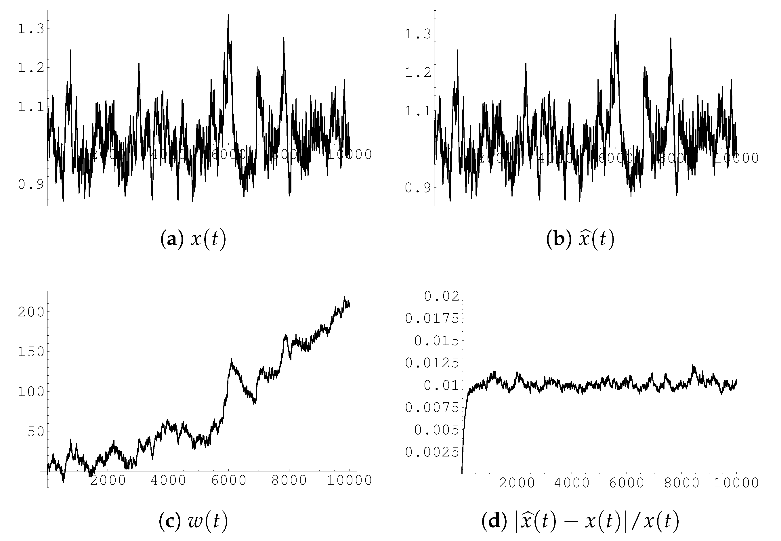
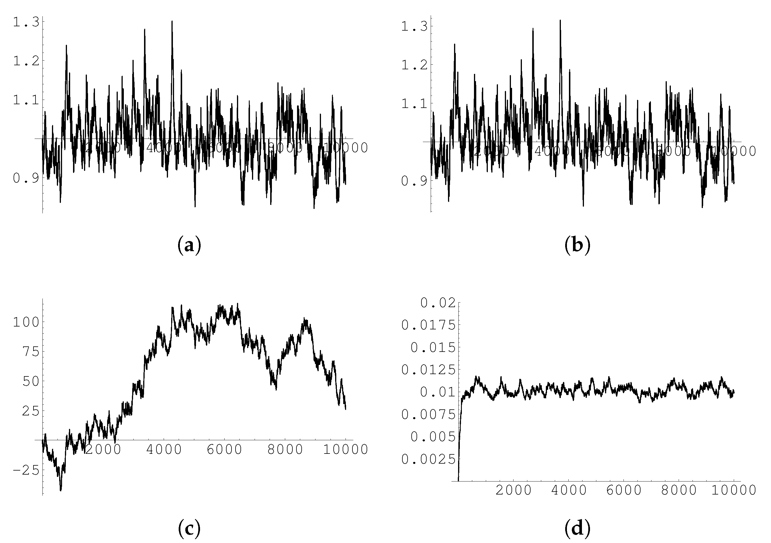
Our previous discussion provides a mathematically rigorous construction of the general solution for the stochastic logistic equation. (Sometimes such a solution, providing explicitly the process $x\left(t\right)$ for each realization of the driving process $w\left(t\right)$ is called a strong solution of the SDE.)

The reader less inclined to mathematically abstract discussions may be willing to have a check that our constructions is indeed reaching its task, e.g., by numerically comparing the solution obtained in this way with a direct numerical solution of the stochastic logistic Equation (28) for the same realization of the driving Wiener process $w\left(t\right)$.

Such a request would be even more justified considering that—quite surprisingly—in the recent literature devoted to symmetry of SDEs and integration of the latter by symmetry method such “numerical check” appear to be completely absent.

We have thus ran a “numerical experiment” consisting of the following procedure (repeated over a number of realizations of the driving process).

• Generate, by means of a random number generator, a sequence of normally distributed $\left(\delta w\right)\left(k\right)$ (for $k=0,...,k_{\max }=k_M$); store these.
• Using the stored values of $\left(\delta w\right)\left(k\right)$, build a discrete-time Wiener process (time step $\delta t$) setting $w\left[0\right]=0$, $w\left[\right(k+1\left)\right]=w\left[k\right]+\left(\delta w\right)\left(k\right)\delta t$; here $w\left[k\right]$ represents the value taken by $w\left(t\right)$ at time $t_k=k\left(\delta t\right)$. Store this.
• Numerically integrate (28), again using the stored $\left(\delta w\right)\left(k\right)$, by setting $x\left(0\right)=x_0$, $x\left[(k+1)\right]=x\left[k\right]+(\alpha x\left[k\right]-\beta x{\left[k\right]}^2)dt+\gamma x\left[k\right]\left(\delta w\right)\left[k\right]$, and store these. Here $x\left[k\right]$ represents the value taken by $x\left(t\right)$ at time $t_k=k\left(\delta t\right)$, for the given realization of $w\left(t\right)$. The values $x\left[k\right]$ represent a bona fide direct numerical solution of our stochastic equation, with the approximation resulting from the finite size of the time step $\left(\delta t\right)$. (We stress we are here using a very basic Euler first order integration scheme, thus have to expect rather poor precision in our numerical results. One could use more refined integration schemes—see e.g., [56] —but the point here is just to have a reference numerical solution to compare our exact solution with.)
• Use the map (72) to determine $y\left(0\right)=y_0$ corresponding to the assigned initial value $x_0$. Using the stored values of $w\left[k\right]$ (i.e., of $w\left(t\right)$ for the given realization), build $y\left(t\right)$ by means of (75), i.e., setting $y\left[0\right]=y_0$ and $y[k+1]=y\left[0\right]-\beta exp(A{t}_k+\gamma w\left[k\right])\delta t$; here again $y\left[k\right]$ represents the value taken by $y\left(t\right)$ at time $t_k$. The values $y\left[k\right]$ are stored and represent a bona fide direct numerical solution of our equivalent stochastic Equation (75), i.e., of (77); again with the to approximation due to finite size of $\delta t$.
• Use now the inverse map (73) to generate from the values stored in Y—i.e., from $y\left(t\right)$—values $\widehat{x}\left[k\right]$ which represent the values taken by a stochastic process $\widehat{x}\left(t\right)$ at time $t_k$.
• If our procedure is correct, the stochastic process $\widehat{x}\left(t\right)$ is the solution to the Equation (28) for the given realization of $w\left(t\right)$, i.e., should correspond to $x\left(t\right)$ computed directly before. Thus we compare the strings $x\left[k\right]$ and $\widehat{x}\left[k\right]$.

We stress that one expects some disagreement to be present due to the numerical errors and above all to the finite size of the considered time step of the numerical integration. It would be possible to reduce these by considering a more refined numerical integration scheme, but this is not of interest here: we only want to check that our procedure is correct in that it does indeed produce a solution to the equation under study, and this is clearly shown by our rough numerical computations.

The results of these numerical experiments are shown (for four—randomly chosen—given realizations of the driving process; we have of course conducted many runs) in Figure 1, Figure 2, Figure 3 and Figure 4 (see captions there for details), and confirm that indeed our procedure provides a correct solution to the stochastic logistic equation for each realization of the driving Wiener process (the disagreement between x and $\widehat{x}$ remains within a few percent over 10.000 time steps).

9. Conclusions

We have first considered some general aspects of the theory of symmetry for deterministic differential equations [1,2,3,4,5,6,7,8], focusing in particular on ODEs; and we have recalled the key features of the extension of this theory to the realm of (ordinary) stochastic differential equations [9,10,11,12,13,14,15,16,17,18,19,20,21,22,23,24,25,26,27,28,29,30,31,32,33,34,35,36].

We have then considered as a case study the stochastic logistic Equation (23), i.e., the logistic equation with different types of noise: environmental, demographical, and both of these, i.e., in the so called complete model. We have been searching for symmetries of these equations, and in particular for simple standard or W-symmetries; according to the general theory of symmetries of SDEs, these would allow to explicitly integrate the equation.

By explicit computations, based on solving the determining Equations (9) and (10) for standard or W-symmetries, we have seen that of demographical noise (Section 6) and in the case of the complete model (Section 7), the SLE admits no symmetries. The same holds for the SLE with non-constant environmental noise (Section 5.4). On the other hand, we found that in the case of constant environmental noise the SLE has symmetries, as shown in Section 5.

In this latter case, we have applied the general theory, proceeding to the integration of the SLE through use of symmetry-adapted variables. We have also conducted some numerical computation to support our conclusions in this case.

This has also allowed to better understand the meaning of the (symmetry-based, in this case) integration procedure for stochastic equations: we are able, for each realization of the underlying Wiener process $w\left(t\right)$, to explicitly exhibit the corresponding realization of the stochastic process $x\left(t\right)$ described by the SDE.