Space-Time Inversion of Stochastic Dynamics

Abstract

This article introduces the concept of space-time inversion of stochastic Langevin equations as a way of transforming the parametrization of the dynamics from time to a monotonically varying spatial coordinate. A typical physical problem in which this approach can be fruitfully used is the analysis of solute dispersion in long straight tubes (Taylor-Aris dispersion), where the time-parametrization of the dynamics is recast in that of the axial coordinate. This allows the connection between the analysis of the forward (in time) evolution of the process and that of its exit-time statistics. The derivation of the Fokker-Planck equation for the inverted dynamics requires attention: it can be deduced using a mollified approach of the Wiener perturbations “a-la Wong-Zakai” by considering a sequence of almost everywhere smooth stochastic processes (in the present case, Poisson-Kac processes), converging to the Wiener processes in some limit (the Kac limit). The mathematical interpretation of the resulting Fokker-Planck equation can be obtained by introducing a new way of considering the stochastic integrals over the increments of a Wiener process, referred to as stochastic Stjelties integrals of mixed order. Several examples ranging from stochastic thermodynamics and fractal-time models are also analyzed.

1. Introduction

Statistical mechanics is deeply intertwined with stochastic methods since the pioneering contributions by Einstein and Smoluchowski that have foreseen the need of complementing the classical thermodynamic approach based on average quantities with a detailed understanding of fluctuation statistics [1,2]. The understanding of the statistical properties of fluctuations characterizing particle motion in colloidal systems, both in equilibrium and non-equilibrium conditions, has recently achieved a considerable experimental support from micro- and nanoscale analysis of the motion of single particles both in gaseous and liquid systems [3,4,5]. These experiments have shown that at short-time scales, Brownian fluctuations appear more regular than what predicted by the classical Langevin-Wiener paradigm [6,7].

Closely related to the experimental analysis, the research on stochastic methods in physics is experiencing a renewed flourishing in a variety of different directions: from the understanding of the emergent anomalous features in a variety of physical systems showing both subdiffusive and superdiffusive scalings [8,9], to the understanding of weak ergodicity breaking [10,11], to the characterization of stochastic processes possessing finite propagation velocity [12,13,14,15] and the understanding of the thermodynamic implications of this property [16,17,18,19,20]. Stochastic processes possessing bounded propagation velocity intrinsically arise in relativistic theories [21,22,23,24] and in applications involving both high-energy physics and astrophysical models [25].

In this article, starting from a classical fluid dynamic problem, namely particle dispersion in a channel flow [26], we analyze some novel physical and mathematical implications of it associated with the need of reparametrizing stochastic particle motion with respect to a characteristic spatial coordinate instead of the physical time. For details see Section 3. This problem stems from the possibility of defining two different moment hierarchies (spatial and temporal) [27,28,29,30] and is motivated by the interest in obtaining an analytical representation of their mutual relationships. A strategy for achieving this scope is the parametrization of the particle motion with respect to the axial coordinate, instead of the physical time (which is the natural setting for the particle Langevin equation), see Section 2.

For this reason, we refer to this approach as “the space-time inversion” of stochastic dynamics. Space-time inversion provides for some classes of stochastic dynamics a way to treat time and some specific spatial coordinate on equal footing, and space-time inversion provides the mathematical formulation for this symmetry.

Albeit from the strictly mathematical point of view, space-time inversion is a purely stochastic subordination [31,32]—and subordination and time change is a well known technique in the theory of stochastic processes [33,34], widely applied in statistical physics in connection with modulations of Continuous Time Random Walk models [35,36]—its solution, for nonlinear Langevin equations is far from trivial and of interest in the much broader context of stochastic methodsin physics. In point of fact, it is shown in Section 4 that none of the classical stochastic formulations (Ito, Stratonovich, Hänggi-Klimontovich, $\lambda$-integrals) of stochastic calculus [37] is able to interpret the correct inversion formula, which requires the introduction of the concept of stochastic integrals of mixed order, see Section 5. Moreover, space-time inversion may find application in a variety of physical problems as it intrinsically provides the connection between the solution of the forward Fokker-Planck equation and the first-transit transit time probability density function (see Section 6).

With respect to a classical time-change, that is a generic and abstract reparametrization of time, enabling the definition of new families of stochastic processes [34], the space-time inversion of Langevin equations originates from a transport problem and admits a variety of physical implications. For this reason, we follow in this article an approach that may sound “non-rigorous” for the pure mathematician, as oriented to the solution of transport problems via stochastic methods. Nevertheless, we believe that the main novel concepts addressed in the article can be further elaborated and polished without great difficulty, to reach the level of a mathematical theory.

In this article we develop the setting of the space-time inversion problem, and derive the correct “inverted” Langevin equation starting from stochastic processes possessing finite propagation velocity (Poisson-Kac processes) and converging to Wiener processes in the Kac limit [16,19,38,39,40]. This can be viewed as a mollification in the spirit of the Wong-Zakai theorem [41,42]. The interpretation of the resulting Fokker-Planck equation for the probability density leads to introduce the concept of stochastic integrals of mixed order, Section 5. Several physical applications are also briefly outlined, ranging from stochastic thermodynamics to the Langevin modelling of stochastic processes in a “fractal time” [43,44].

2. Basic Definitions and Statement of the Problem

Consider a stochastic process $\mathbf{X}\left(t\right)=(X_1\left(t\right),\dots ,X_n\left(t\right))$ in ${\mathbb{R}}^n$ defined by the generalized Langevin equation

$$d{x}_h\left(t\right)=f_h(\mathbf{x}\left(t\right),t)dt+{\displaystyle \sum _{\alpha =1}^s}{a}_{h,\alpha }(\mathbf{x}\left(t\right),t)d{w}_{s,\alpha }\left(t\right),$$

(1)

$h=1,\dots ,n$, where $f_h(\mathbf{x},t)$ are the entries of a deterministic vector field, and $d{w}_{s,\alpha }\left(t\right)$, $\alpha =1,\dots ,s$ the increments of the stochastic processes $w_{s,\alpha }\left(t\right)$, which do not need to be necessarily of Wiener nature. In Equation (1), the lower case symbols $x_h\left(t\right)$ indicate the realizations of $X_h\left(t\right)$.

Assume that, for some h, say $h=1$, $a_{1,\alpha }=0$ identically, for all $\alpha =1,\dots ,s$, and that $f_1(\mathbf{x},t)\ge 0$ for any value of $\mathbf{x}$ and t. Under these conditions, $x_1\left(t\right)=x_{1,0}+{\int }_0^t{f}_1(\mathbf{x}\left(\tau \right),\tau )d\tau$ is a monotonic function of t. This means that it would be possible in principle to parametrize the system of Equation (1) with respect to $x_1$ instead of the physical time t. This observation leads to the following definition:

Definition 1.

A stochastic process $X\left(t\right)$ is positively subordinated to the process $Y\left(t\right)$ if there exists a positive function $f(x,y)>0$, such that the following relation holds for the realizations of the two processes

$$dx\left(t\right)=f\left(x\right(t),y(t\left)\right)dt.$$

(2)

Observe that, in Definition 1, the relation between $X\left(t\right)$ and $Y\left(t\right)$ is “ab initio” expressed in terms of the differentials and not as a mathematical equality $x\left(t\right)=\tilde{f}\left(y\left(t\right)\right)$. The latter position would have induced a completely different expression for the differential $dx\left(t\right)$, depending on the dynamics of $Y\left(t\right)$ and on the stochastic calculus considered, (for instance, considering the Ito integral and enforcing the Ito’s lemma [37]).

Assume that the dynamics of $X\left(t\right)$ is positively subordinated to $Y\left(t\right)$ which, in turn, satisfies the stochastic dynamics

$$dy\left(t\right)=g(x\left(t\right),y\left(t\right))dt+a(x\left(t\right),y\left(t\right))d{w}_s\left(t\right).$$

(3)

Enforcing the monotonic relation between $x\left(t\right)$ and t deriving from Equation (2) it is possible to represent the stochastic dynamics (2)–(3) in the form

$$\begin{array}{ccc}\hfill dt& =& h(x,y(x\left)\right)dx\hfill \\ \hfill dy\left(x\right)& =& \overline{g}(x,y\left(x\right))dx+\overline{a}(x,y\left(x\right))d{\overline{w}}_s\left(x\right),\hfill \end{array}$$

(4)

that is, parametrizing the subordinating y-dynamics with respect to x instead of time t. In Equation (4), $h(x,y)=1/f(x,y)$, while the functions $\overline{g}(x,y)$, $\overline{a}(x,y)$ and the stochastic process ${\overline{W}}_s\left(x\right)$ should be determined by a consistency condition connecting Equations (2)–(3) to Equation (4). More precisely, let

$$\begin{array}{ccc}x\left(t\right)& =& x_0+{\int }_{t_0}^{t}f(x\left(\tau \right),y\left(\tau \right))d\tau =F_1(t;t_0,x_0,y_0)\hfill \\ y\left(t\right)& =& y_0+{\int }_{t_0}^{t}g(x\left(\tau \right),y\left(\tau \right))d\tau +{\int }_{t_0}^{t}a(x\left(\tau \right),y\left(\tau \right))d{w}_s\left(\tau \right)=G_1(t;t_0,x_0,y_0),\hfill \end{array}$$

(5)

equipped with some prescription on the meaning of the stochastic Stieltjes integral entering the second Equation (5). The consistency condition, implies that it would be possible to define two functions $\overline{g}(x,y)$, $\overline{a}(x,y)$, and a stochastic process ${\overline{W}}_s\left(x\right)$, such that

$$G_1(t;t_0,x_0,y_0)=y_0+{\int }_{x_0}^{F_1(t;t_0,x_0)}\overline{g}(\xi ,y\left(\xi \right))d\xi +{\int }_{x_0}^{F_1(t;t_0,x_0)}\overline{a}(\xi ,y\left(\xi \right))d{\overline{w}}_s\left(\xi \right).$$

(6)

Therefore, we have the following definition:

Definition 2.

If there exist two functions $\overline{g}(x,y\left(x\right))$ and $\overline{a}(x,y\left(x\right))$, and a stochastic process ${\overline{W}}_s\left(x\right)$ satisfying Equation (6) almost everywhere in t with probability 1, the stochastic dynamics (4) is referred to as the space-time inversion of the Equations (2)–(3).

3. The Prototypical Model

Let us introduce space-time inversion of Langevin equations from physical grounds. The prototypical physical problem motivating this formulation in stochastic dynamics is solute dispersion in a straight channel in the presence of an incompressible Poiseuille flow and diffusion (Taylor-Aris dispersion) [26].

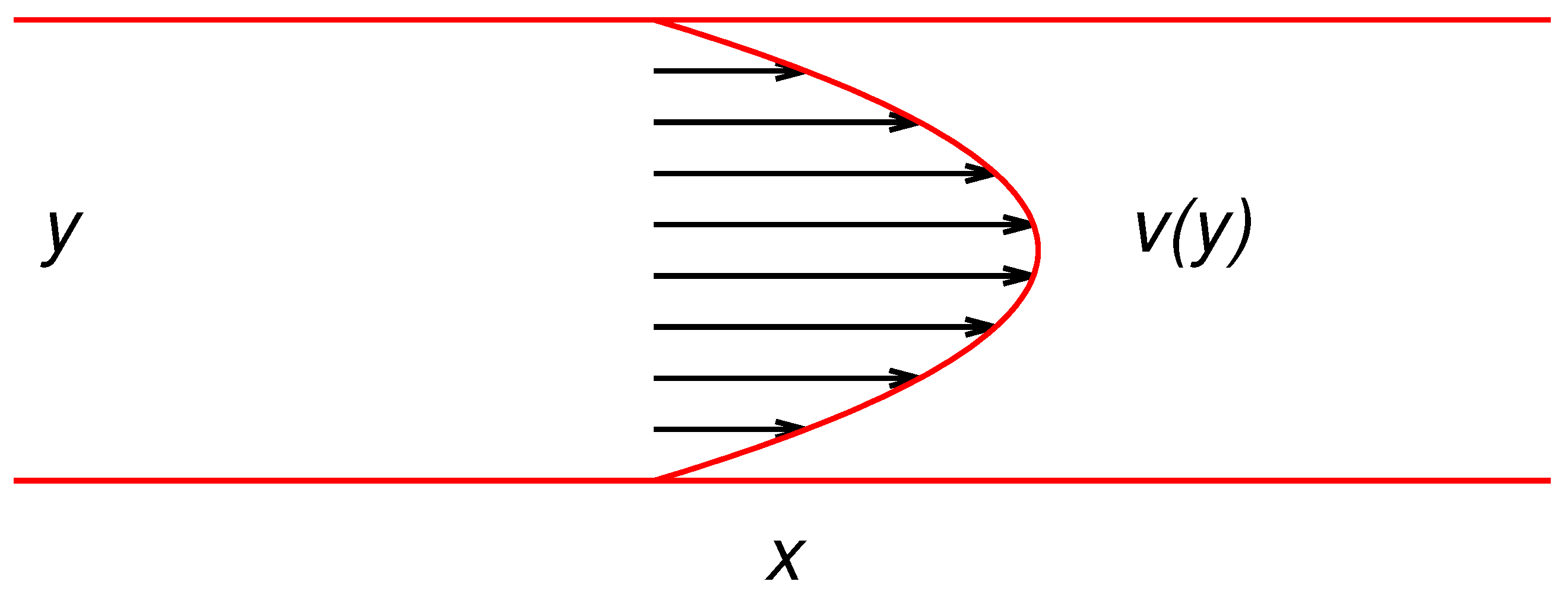
For notational simplicity, consider a two-dimensional model, letting x and y be respectively the axial and the transversal (cross-sectional) coordinates in the channel. A cartoon picture of this problem is sketched in Figure 1.

Solute particles, initially injected in the channel, undergoes advection controlled by the axial Poiseuille flow and diffusion. Particle motion is thus described in non-dimensional form by the equation

$$\begin{array}{ccc}\hfill dx\left(t\right)& =& v\left(y\left(t\right)\right)dt+\sqrt{2K_0{\delta }_x\left(y\left(t\right)\right)}\circ d{w}_1\left(t\right)\hfill \\ \hfill dy\left(t\right)& =& \sqrt{2K_0{\delta }_y\left(y\left(t\right)\right)}\circ d{w}_2\left(t\right),\hfill \end{array}$$

(7)

$x\in (-\infty ,\infty )$, $y\in (0,1)$, where $v\left(y\right)$ is the axial velocity depending solely on the transverse coordinate, $K_0=1/\mathrm{Pe}$ the reciprocal of the Peclét number $\mathrm{Pe}=V_{c}W/D$, corresponding to the ratio of the characteristic diffusion time $W^2/D$ and the characteristic advection time $W/V_c$, where W is the channel width, $V_c$ a characteristic velocity (e.g., the mean velocity), and D the Stokes-Einstein diffusion coefficient. In Equation (7), $W_1\left(t\right)$ and $W_2\left(t\right)$ are two independent Wiener processes. The symbol “○” indicates that the Stratonovich recipe to stochastic calculus is considered. Observe from Equation (7) that both the axial $D_x$ and the transversal diffusivities $D_y$ are considered to be explicitly dependent on the transversal coordinate, that is, on the distance from the walls, $D_x\left(y\right)=K_0{\delta }_x\left(y\right)$, $D_y\left(y\right)=K_0{\delta }_y\left(y\right)$, where obviously ${\delta }_x\left(y\right),{\delta }_y\left(y\right)>0$. For this reason, this problem is referred to as the generalized Taylor-Aris problem. Position dependent diffusivities occur in micrometric channels when the particle size is comparable to W [4,45,46]. As regards the flow velocity, Poiseuille conditions in a 2d channel dictates a parabolic profile $v\left(y\right)=6y(1-y)$ (in this case $V_c$ is just the mean velocity). To avoid singularity issues at the walls, we consider a slip perturbation of the Poiseuille profile, namely $v\left(y\right)=6y(1-y)+\epsilon >0$, where $\epsilon$ is a small slip velocity. The Poiseuille transport problem can be recovered in the limit for $\epsilon \to 0$. Equation (7) are complemented with reflection conditions at the channels walls located at $y=0,1$.

If the Peclét number is sufficiently high, $Pe>{10}^2$ (which is the rule in particle transport problems), axial diffusion can be neglected as the dominant contribution to axial transport is essentially convective. Therefore, setting $a\left(y\right)={\delta }_y\left(y\right)$, $W\left(t\right)=W_2\left(t\right)$ Equation (7) simplifies as follows

$$\begin{array}{ccc}\hfill dx\left(t\right)& =& v\left(y\right(t\left)\right)dt\hfill \\ \hfill dy\left(t\right)& =& \sqrt{2K_{0}a\left(y\left(t\right)\right)}\circ dw\left(t\right).\hfill \end{array}$$

(8)

If wall effects to diffusion are negligible, then $a\left(y\right)=1$, and the specification of the stochastic calculus adopted becomes unnecessary.

Since $v\left(y\right)>0$, it is natural to ask whether it would be possible to parametrize transversal motion with respect to the axial coordinate, which corresponds to the space-time inversion problem introduced in the previous Section.

4. Mollified Description and Space-Time Inverse Langevin Equation

The space-time inversion problem for Equation (8) can be approached by considering the mollification of the stochastic dynamics using Poisson-Kac processes [17,38], namely,

$$\begin{array}{ccc}\hfill dx\left(t\right)& =& v\left(y\right(t\left)\right)dt\hfill \\ \hfill dy\left(t\right)& =& b_0\beta \left(y\left(t\right)\right){(-1)}^{\chi (t;\lambda )}dt,\hfill \end{array}$$

(9)

where $b_0$ and $\lambda$ are positive parameters such that $b_0^2/2\lambda =K_0$, and $\beta \left(y\right(t\left)\right)$ is defined by ${\beta }^2\left(y\right)=a\left(y\right)$. In Equation (9), $\chi (t;\lambda )$ is a Poisson process characterized by the uniform transition rate $\lambda >0$. The Wiener limit, that is, Equation (8) interpreted within the Stratonovich calculus is recovered in the Kac limit, that is, for $b_0,\lambda \to \infty$ keeping fixed the ratio $b_0^2/2\lambda =K_0$. Equation (9) with respect to Equation (8) can be viewed as a mollification “a-la Wong-Zakai” [41,42], in which the singularity structure of the Wiener perturbation is “cured” by using a piecewise smooth and Lipshitz continuous stochastic process. The only technical difference is that, while in the original Wong-Zakai mollification, a piecewise interpolation of the Wiener process has been adopted, here Poisson-Kac process are considered.

Proposition 1.

In the Kac limit, the overall probability density function $p(x,y;t)$ associated with the stochastic process (9) is a solution of the Fokker-Planck equation associated with the Wiener-Stratonovich Langevin Equation (8).

Proof. 

The overall probability density function associated with Equation (9) is given by $p(x,y;t)=p_{+}(x,y;t)+p_{-}(x,y;t)$ where the two partial probability densities $p_{\pm }(x,y,t)$ satisfy the hyperbolic system of equations

$$\begin{array}{ccc}\hfill {\partial }_t{p}_{\pm }(x,y;t)& =& -{\partial }_x\left[v\left(y\right)p_{\pm }(x,y;t)\right]\mp b_0{\partial }_y\left[\beta \left(y\right)p_{\pm }(x,y;t)\right]\hfill \\ & \mp & \lambda \left[p_{+}(x,y;t)-p_{-}(x,y;t)\right]\hfill \end{array}$$

(10)

where ${\partial }_{\xi }=\partial /\partial \xi$, $\xi =t,x,y$. Consequently, $p(x,y;t)$ is a solution of the conservation equation

$${\partial }_{t}p(x,y;t)=-{\partial }_x\left[v\left(y\right)p(x,y;t)\right]-{\partial }_y\left[\beta \left(y\right)\varphi (x,y;t)\right]$$

(11)

where $\varphi (x,y;t)=b_0\left[p_{+}(x,y;t)-p_{-}(x,y;t)\right]$ fulfils the equation

$${\partial }_t\varphi (x,y;t)+{\partial }_x\left[v\left(y\right)\varphi (x,y;t)\right]+2\lambda \varphi (x,y;t)=-b_0^2{\partial }_y\left[\beta \left(y\right)p(x,y;t)\right].$$

(12)

In the Kac limit, $b_0,\lambda \to \infty$, corresponding to infinite propagation velocity and vanishing correlation time, keeping fixed the nominal diffusivity $K_0=b_0^2/2\lambda$, Equation (12) provides $\varphi (x,y;t)=-K_0{\partial }_y\left[\beta \left(y\right)p(x,y;t)\right]$ and thus the evolution equation for $p(x,y;t)$ reads

$${\partial }_{t}p(x,y;t)=-{\partial }_x\left[v\left(y\right)p(x,y;t)\right]+K_0{\partial }_y\left[\beta \left(y\right){\partial }_y\left(\beta \left(y\right)p(x,y;t)\right)\right].$$

(13)

Rearranging the last term, considering that ${\beta }^2\left(y\right)=a\left(y\right)$, thus $a^{\prime }\left(y\right)/2=\beta \left(y\right){\beta }^{\prime }\left(y\right)$, where ${\beta }^{\prime }\left(y\right)=d\beta \left(y\right)/dy$, one finally obtains

$${\partial }_{t}p(x,y;t)=-{\partial }_x\left[v\left(y\right)p(x,y;t)\right]-\frac{K_0}{2}{\partial }_y\left[a^{\prime }\left(y\right)p(x,y;t)\right]+K_0{\partial }_y^2\left[a\left(y\right)p(x,y;t)\right],$$

(14)

which is the Fokker-Planck equation for the probability density function of the process (8) interpreted in the meaning of Stratonovich. □

Next, consider the space-time inversion of Equation (9). The y-dynamics in the inverted model is parametrized with respect to x as

$$dy\left(x\right)=b_0\overline{\beta }\left(y\left(x\right)\right){(-1)}^{\overline{\chi }(x,\overline{\lambda })}dx,$$

(15)

where $\overline{\chi }(x,\overline{\lambda })$ is a Poisson process parametrized with respect to x and characterized by the transition rate $\overline{\lambda }$. Both $\overline{\beta }$ and $\overline{\lambda }$ should be determined by the consistency condition. Observe that in the case of Poisson-Kac processes the consistency condition can be expressed as a local relation a.e. deriving by differentiation of composite functions $dy\left(t\right)/dt={(dy\left(x\right)/dx)}_{x=x\left(t\right)}{(dx/dt)}_{y=y\left(t\right)}$, which implies $b_0\beta \left(y\right){(-1)}^{\chi (t,\lambda )}=b_0\overline{\beta }\left(y\right){(-1)}^{\overline{\chi }(x,\overline{\lambda })}v\left(y\right)$, and thus, $\overline{\beta }\left(y\right)=\beta \left(y\right)/v\left(y\right)$. Next consider the transition probability in the time interval $\Delta t$ which equals $\lambda \Delta t+O(\Delta t^2)$. This quantity is also equal in the inverted representation to $\overline{\lambda }\Delta x+O(\Delta x^2)$, where $\Delta x$ is related to $\Delta t$ by the relation $\Delta x=v\left(y\right)\Delta t$, and consequently $\overline{\lambda }=\lambda /v\left(y\right)$. Observe that for the inverted process the transition rate becomes a function of y. This result is summarized below.

Proposition 2.

The space-time inversion of the Poisson-Kac process (9) is given by

$$\begin{array}{ccc}\hfill dt\left(x\right)& =& \frac{dx}{v\left(y\right(x\left)\right)}\hfill \\ \hfill dy\left(x\right)& =& \frac{b_0\beta \left(y\left(x\right)\right)}{v\left(y\right(x\left)\right)}{(-1)}^{\chi (x,\lambda /v(y\left(x\right))}dx.\hfill \end{array}$$

(16)

Let us analyze the statistical properties of the inverted process (16). It is sufficient to consider the y-process alone, that is, the second Equation (16). Its statistical description involves the two partial probability density functions ${\overline{p}}_{\pm }(y;x)$ that are solution of the hyperbolic system of equations [17,38]

$${\partial }_x{\overline{p}}_{\pm }(y;x)=\mp b_0{\partial }_y\left[\frac{\beta \left(y\right)}{v\left(y\right)}{\overline{p}}_{\pm }(y;x)\right]\mp \frac{\lambda }{v\left(y\right)}\left[{\overline{p}}_{+}(y;x)-{\overline{p}}_{-}(y;x)\right].$$

(17)

Consider the Kac limit of this process: the overall density function $\overline{p}(y;x)={\overline{p}}_{+}(y;x)+{\overline{p}}_{-}(y;x)$ satisfies the equation ${\partial }_x\overline{p}(y;x)=-{\partial }_y\left[\beta \left(y\right)\overline{\varphi }(y;x)/v\left(y\right)\right]$, where $\overline{\varphi }(y;x)=b_0\left[{\overline{p}}_{+}(y;x)-{\overline{p}}_{-}(y;x)\right]$. In the Kac limit, that is, for $b_0,\lambda \to \infty$, keeping fixed the ratio $b_0^2/2\lambda =K_0$, the auxiliary flux variable $\overline{\varphi }(y;x)$ satisfies the constitutive equation

$$\overline{\varphi }(y;x)=-K_{0}v\left(y\right){\partial }_y\left[\frac{\beta \left(y\right)\overline{p}(y;x)}{v\left(y\right)}\right],$$

(18)

and consequently

$${\partial }_x\overline{p}(y;x)=K_0{\partial }_y\left[\beta \left(y\right){\partial }_y\left(\frac{\beta \left(y\right)\overline{p}(y;x)}{v\left(y\right)}\right)\right].$$

(19)

Equation (19) can be further rearranged in terms of the quantities entering the original stochastic model (8). This leads to the following result:

Proposition 3.

The Fokker-Planck equation for the space-time inverted process Equation (8) is given by

$${\partial }_x\overline{p}(y;x)=-\frac{K_0}{2}{\partial }_y\left[\frac{a^{\prime }\left(y\right)}{v\left(y\right)}\overline{p}(y;x)\right]+K_0{\partial }_y^2\left[\frac{a\left(y\right)}{v\left(y\right)}\overline{p}(y;x)\right]$$

(20)

where $a^{\prime }\left(y\right)=da\left(y\right)/dy$.

Proof. 

Reworking by part the r.h.s. of (20) one obtains

$${\partial }_x\overline{p}(y;x)=K_0{\partial }_y^2\left[\frac{{\beta }^2\left(y\right)\overline{p}(y;x)}{v\left(y\right)}\right]-K_0{\partial }_y\left[\frac{{\beta }^{\prime }\left(y\right)\beta \left(y\right)\overline{p}(y;x)}{v\left(y\right)}\right].$$

(21)

Since $\beta \left(y\right)=\sqrt{a\left(y\right)}$, $\beta \left(y\right){\beta }^{\prime }\left(y\right)=a^{\prime }\left(y\right)/2$, and Equation (20) follows. □

The result expressed by Equation (20) is remarkable since:

• for $a\left(y\right)=\mathrm{constant}=1$, Equation (20) provides the classical subordination result [47], corresponding to the dynamics of the space-inverted process given by $dy\left(x\right)=\sqrt{2K_0/v\left(y\left(x\right)\right)}d\overline{w}\left(x\right)$, where $\overline{W}\left(x\right)$ is a Wiener process and this stochastic equation should be interpreted using the Ito prescription;
• if the original Langevin Equation (8) is nonlinear, that is, $a\left(y\right)$ depends explicitly on y, the Fokker-Planck Equation (20) does not correspond to any simple Langevin equation of the form

  $$dy\left(x\right)=\sqrt{\frac{2K_{0}a\left(y\left(x\right)\right)}{v\left(y\right(x\left)\right)}}{\ast }_{\lambda }d\overline{w}\left(x\right),$$

  (22)

  where the stochastic integral is interpreted as a $\lambda$-integral [37] (the symbol “${\ast }_{\lambda }$” indicates this assumption on the stochastic integral), where $\lambda =0$ corresponds to Ito, $\lambda =1/2$ to Stratonovich, $\lambda =1$ to Hänggi-Klimontovich calculus. For the definition of $\lambda$-integrals see Reference [37] and the introductory discussion at the beginning of the Section 5.

Let us consider some numerical examples. Consider the stochastic model (8) for a Poiseuille flow $v\left(y\right)=6y(1-y)+\epsilon$ in $y\in [0,1]$, where the small slip contribution $\epsilon ={10}^{-2}$ is added for ensuring positive subordination, and $K_0={10}^{-3}$. As regards $a\left(y\right)$ two models are considered: (model I) where $a\left(y\right)=a_1+y/(a_2+y)$, $a_1={10}^{-2}$, $a_2=5$, and (model II) where $a\left(y\right)=a_1+cos\left(2\pi a_{2}y\right)$, $a_1=1.1$, and $a_2=5$. Stochastic simulations of Equation (8) involve an ensemble of $N_p={10}^4$ particles initially (i.e., at time $t=0$) located at $x=0$ and uniformly distributed on the transversal cross section $y\in [0,1]$. In order to reach a stationary hitting distribution at a constant axial abscissa x, it is sufficient to consider $x>k_{\min }=3000$. Once the particle reach integer values k of the axial abscissa greater than $k_{\min }$, the value of the transversal abscissa y at the transit point is recorded. 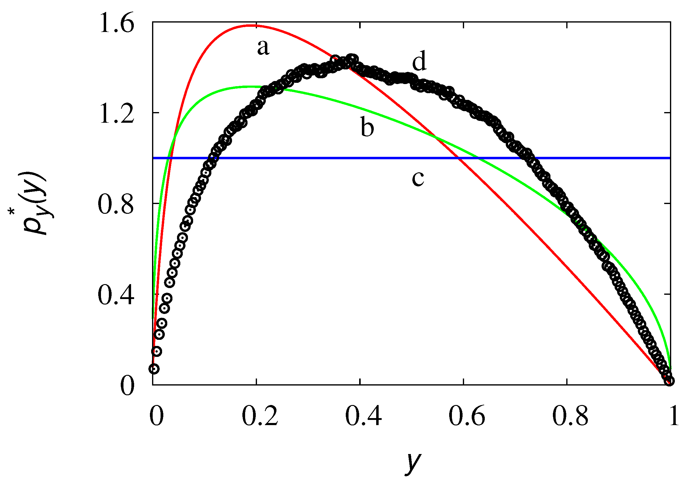By considering a set of k values of the axial abscissa for evaluating the intersection, that is, $k=k_{\min }+1,\dots ,2k_{\min }$, it is possible to estimate the stationary transversal distribution of the transit point averaged over ∼${10}^7$–${10}^8$ realization still using a relatively small ensemble of particles. 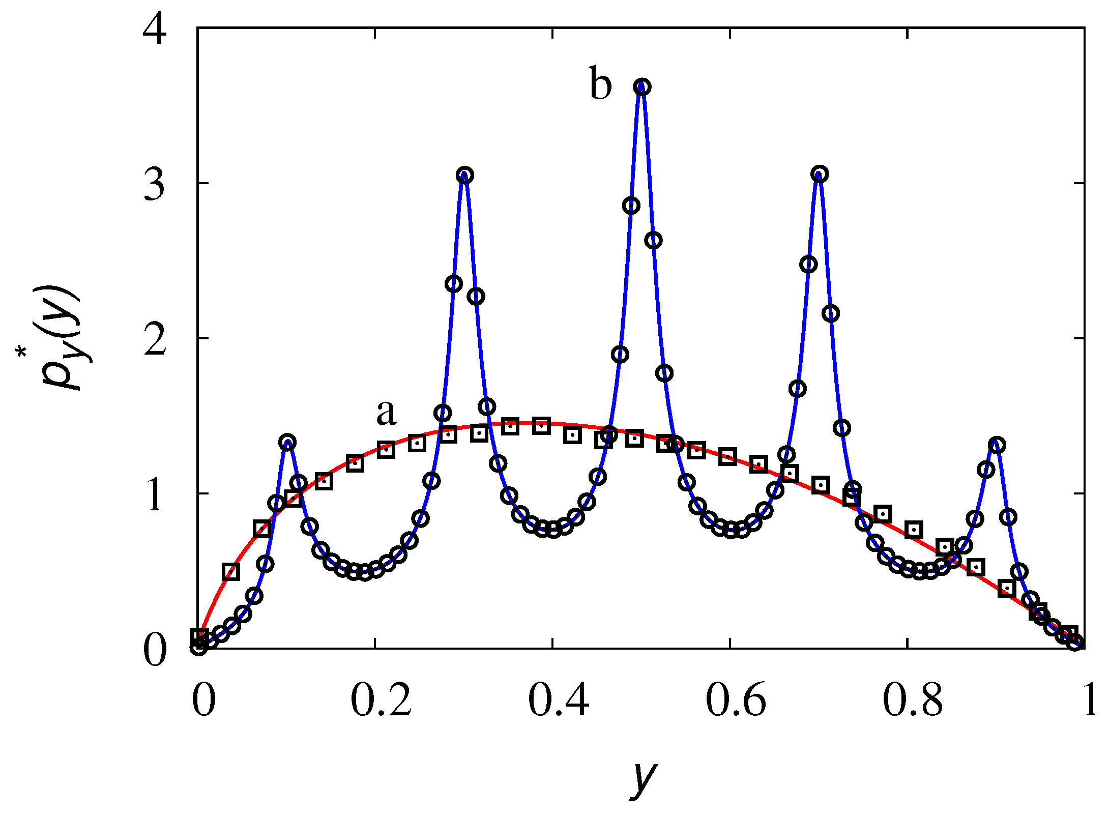From Equation (19), or equivalently Equation (20), the stationary transversal transit distribution ${\overline{p}}^{*}\left(y\right)$ is given by

$${\overline{p}}^{*}\left(y\right)=A\frac{v\left(y\right)}{\sqrt{a\left(y\right)}},$$

(23)

where A is the normalization constant. Figure 2 depicts the results of the stochastic simulations, using the direct stochastic model (8) (symbols) and the theoretical predictions (23) (solid lines) for model I and model II, revealing the agreement between the theoretical results for the space-time inverted process and the stochastic simulations of the direct dynamics.

The stationary transversal hitting distribution cannot be reproduced from any stochastic interpretation of the inverse stochastic dynamics of the form (22). This claim is depicted in Figure 3 for model I (data of Figure 2) where the stationary transversal hitting distribution associated with Equation (22), and expressed by ${\overline{p}}^{*}\left(y\right)=A{[v\left(y\right)/a\left(y\right)]}^{1-\lambda }$, are compared, for typical values of $\lambda$, with the direct stochastic simulations of Equation (8).

5. Mixed-Order Stochastic Integrals

From the above analysis, it follows naturally the quest for defining an appropriate space-time inverted Wiener-driven Langevin equation for the process defined by Equation (8), providing the Fokker-Planck Equation (20) as the evolution equation for its probability density function $\overline{p}(y;x)$.

In point of fact, the Fokker-Planck Equation (20) can be derived from a stochastic Wiener-driven Langevin equation by introducing a generalization of the stochastic integrals. The classical approach to stochastic Stieltjes integrals is grounded on the concept of $\lambda$-integrals [37], corresponding to an evaluation of the integrand at a convex mean of the endpoint values of its argument at each subinterval.

Let us briefly review this concept. Consider a realization w of a Wiener process, and let $f\left(w\right)$ a function of it. The stochastic Stieltjes integral of $f\left(w\right)$ with respect to the increments of w, in the interval $[a,b]$, can be performed in different ways. It is usually referred to as $\lambda$-integral and indicated with the symbol ${\int }_a^{b}f\left(w\right){\ast }_{\lambda }dw$, where $\lambda \in [0,1]$. A $\lambda$-integral of $f\left(w\right)$ with respect to $dw$ can be defined by considering a subdivision ${\left\{t_i\right\}}_{i=1}^N$ of $[a,b]$, $t_0=a$, $t_i<t_{i+1}$, $t_N=b$, $\delta ={max}_i|t_i-t_{i-1}|$, as

$${\int }_a^{b}f\left(w\right){\ast }_{\lambda }dw=\underset{\delta \to 0}{lim}{\displaystyle \sum _{i=1}^N}f(\lambda w_i+(1-\lambda )w_{i-1})\Delta w_i$$

(24)

where $w_i=w\left(t_i\right)$, $\Delta w_i=w_i-w_{i-1}$. For $\lambda =0,1/2,1$, one recovers the Ito, Stratonovich and Hänggi-Klimontovich formulation of stochastic integration, respectively. The Hänggi-Klimontovich formulation finds application in some statistical mechanical approaches to the kinetic equation and to fluctuation phenomena [48].

Next, consider the stochastic integration of the product of two functions, say $f\left(w\right)$ and $g\left(w\right)$ with respect to the increments of w. It is possible to introduce a generalization of the $\lambda$-integrals by considering the mixed $(\lambda ,\mu )$-integrals, $\lambda ,\mu \in [0,1]$ as

$${\int }_a^{b}f\left(w\right)g\left(w\right){\ast }_{\lambda ,\mu }dw=\underset{\delta \to 0}{lim}{\displaystyle \sum _{i=1}^N}f(\lambda w_i+(1-\lambda )w_{i-1})g(\mu w_i+(1-\mu )w_{i-1})\Delta w_i,$$

(25)

where the same notation used in Equation (24) has been adopted. Essentially, in mixed $(\lambda ,\mu )$-integrals, two different recipes in the evaluation of the two integrand functions $f\left(w\right)$ and $g\left(w\right)$ are chosen. We leave to further analysis the detailed description of the property of this mathematical tool, as the main focus in the present context is to show that the Fokker-Planck Equation (20) can be derived starting from a generalization of the Langevin Equation (22) involving the use of mixed stochastic integrals.

Specifically, consider the following generalized Langevin equation

$$dy\left(x\right)=\frac{N\left(y\right(x\left)\right)}{D\left(y\right(x\left)\right)}{\ast }_{\mu }^{\lambda }d\overline{w}\left(x\right),$$

(26)

with $D\left(x\right)>0$, and where $d\overline{w}\left(x\right)$ is the increment of a Wiener process parametrized with respect to x in the interval $(x,x+dx)$, equipped with the initial condition

$$y\left(x_0\right)=y_0$$

(27)

In Equation (26) the symbol “${\ast }_{\mu }^{\lambda }$” indicates that this stochastic differential equation should be meant with respect to a mixed theory of stochastic integration. The formal solution of Equations (26)–(27) is

$$y\left(x\right)=y_0+{\int }_{x_0}^x\frac{N\left(y\left(x^{\prime }\right)\right)}{D\left(y\left(x^{\prime }\right)\right)}{\ast }_{\mu }^{\lambda }dw\left(x^{\prime }\right),$$

(28)

where the symbol “${\ast }_{\mu }^{\lambda }$” indicates that the mixed integral at the r.h.s of Equation (28) refers of a $\lambda$-parametrization of the numerator $N\left(y\right(x\left)\right)$ and to a $\mu$-parametrization of the denominator $D\left(y\right(x\left)\right)$.

It is not difficult, using “a physicist approach”, to derive the associated Fokker-Planck equation (a rigorous mathematical formulation can be developed in a later stage) as,

$$\begin{array}{ccc}\hfill dy\left(x\right)& =& \frac{N\left(y\right(x\left)\right)}{D\left(y\right(x\left)\right)}{\ast }_{\mu }^{\lambda }d\overline{w}\left(x\right)=\frac{N\left(y\right(x)+\lambda dy(x\left)\right)}{D\left(y\right(x)+\mu dy(x\left)\right)}d\overline{w}\left(x\right)\hfill \\ & =& \frac{N\left(y\left(x\right)\right)+\lambda N^{\prime }\left(y\left(x\right)\right)dy\left(x\right)+o\left(d{x}^{1/2}\right)}{D\left(y\left(x\right)\right)+\mu D^{\prime }\left(y\left(x\right)\right)dy\left(x\right)+o\left(d{x}^{1/2}\right)}d\overline{w}\left(x\right)\hfill \\ & =& \frac{N(y\left(x\right)+\lambda N^{\prime }\left(y\left(x\right)\right)dy\left(x\right)+o\left(d{x}^{1/2}\right)}{D\left(y\left(x\right)\right)\left[1+\mu D^{\prime }\left(y\left(x\right)\right)/D\left(y\left(x\right)\right)dy\left(x\right)+o\left(d{x}^{1/2}\right)\right]}d\overline{w}\left(x\right)\hfill \\ & =& \frac{1}{D\left(x\right)}\left[N(y\left(x\right)+\lambda N^{\prime }\left(y\left(x\right)\right)dy\left(x\right)+o\left(d{x}^{1/2}\right)\right]\hfill \\ & \times & \left[1-\mu \frac{D^{\prime }\left(y\left(x\right)\right)}{D\left(y\right(x\left)\right)}dy\left(x\right)+o\left(d{x}^{1/2}\right)\right]d\overline{w}\left(x\right),\hfill \end{array}$$

(29)

where $o\left(d{x}^{1/2}\right)$ indicates a quantity vanishing to zero for $dx\to 0$ faster than $d{x}^{1/2}$, and $N^{\prime }\left(y\left(x\right)\right)$, $D^{\prime }\left(y\left(x\right)\right)$ represent the derivatives of these functions with respect to their argument, $N^{\prime }{\left(y\left(x\right)\right)=dN\left(\xi \right)/d\xi |}_{\xi =y\left(x\right)}$, and analogously for $D^{\prime }\left(y\left(x\right)\right)$.

The increments $dy\left(x\right)$ at the r.h.s of Equation (29) can be expanded to the leading order, and this corresponds to treat Equation (26) in its Ito formulation $dy\left(x\right)=\left[N\left(y\right(x\left)\right)/D\left(y\right(y\left(x\right))\right]d\overline{w}\left(x\right)$. Consequently, Equation (29) becomes

$$\begin{array}{ccc}\hfill dy\left(x\right)& =& \frac{N\left(y\right(x\left)\right)}{D\left(y\right(x\left)\right)}d\overline{w}\left(x\right)+\frac{1}{D\left(y\right(x\left)\right)}\left[\lambda N^{\prime }\left(y\left(x\right)\right)-\mu \frac{N\left(y\left(x\right)\right)D^{\prime }\left(y\left(x\right)\right)}{D\left(y\right(x\left)\right)}\right]dy\left(x\right)d\overline{w}\left(x\right)+o\left(dx\right)\hfill \\ & =& \frac{N\left(y\right(x\left)\right)}{D\left(y\right(x\left)\right)}d\overline{w}\left(x\right)+\frac{1}{D\left(y\right(x\left)\right)}\left[\lambda N^{\prime }\left(y\left(x\right)\right)-\mu \frac{N\left(y\left(x\right)\right)D^{\prime }\left(y\left(x\right)\right)}{D\left(y\right(x\left)\right)}\right]\frac{N\left(y\right(x\left)\right)}{D\left(y\right(x\left)\right)}d{\overline{w}}^2\left(x\right),\hfill \end{array}$$

(30)

where in the last expression the higher order term $o\left(dx\right)$ has been neglected. Since $d^2\overline{w}\left(x\right)=dx$ [49], Equation (30) corresponds to the equivalent Langevin-Ito equation

$$\begin{array}{ccc}\hfill dy\left(x\right)& =& \frac{1}{D\left(y\right(x\left)\right)}\left[\lambda N^{\prime }\left(y\left(x\right)\right)-\mu \frac{N\left(y\left(x\right)\right)D^{\prime }\left(y\left(x\right)\right)}{D\left(y\right(x\left)\right)}\right]\frac{N\left(y\right(x\left)\right)}{D\left(y\right(x\left)\right)}dt+\frac{N\left(y\right(x\left)\right)}{D\left(y\right(x\left)\right)}d\overline{w}\left(x\right)\hfill \\ & =& V_{\mathrm{eff}}\left(y\left(x\right)\right)dt+\frac{N\left(y\right(x\left)\right)}{D\left(y\right(x\left)\right)}d\overline{w}\left(x\right),\hfill \end{array}$$

(31)

where

$$V_{\mathrm{eff}}\left(y\left(x\right)\right)=\frac{1}{D\left(y\right(x\left)\right)}\left[\lambda N^{\prime }\left(y\left(x\right)\right)-\mu \frac{N\left(y\left(x\right)\right)D^{\prime }\left(y\left(x\right)\right)}{D\left(y\right(x\left)\right)}\right]\frac{N\left(y\right(x\left)\right)}{D\left(y\right(x\left)\right)}.$$

(32)

The corresponding Fokker-Planck equation for the associated probability density function $\overline{p}(y;x)$ is therefore

$$\frac{\partial \overline{p}(y;x)}{\partial x}=-\frac{\partial \left[V_{\mathrm{eff}}\left(y\right)\overline{p}(y;x)\right]}{\partial y}+\frac{1}{2}\frac{{\partial }^2}{\partial y^2}\left[\frac{N^2\left(y\right)}{D^2\left(y\right)}\overline{p}\left(yx\right)\right].$$

(33)

It is easy to see that for $\mu =\lambda$ Equations (32) provides the result obtained from a classical $\lambda$-parametrization of the stochastic integral, namely,

$$V_{\mathrm{eff}}\left(y\right)=\lambda \frac{N\left(y\right)}{D\left(y\right)}\frac{d}{dy}\left(\frac{N\left(y\right)}{D\left(y\right)}\right),$$

(34)

which is a consequence of the fact that a mixed $(\lambda ,\lambda )$-integral is indeed a $\lambda$-integral. The above analysis provides the analytical background for the following result.

Proposition 4.

Equation (20) represents the Fokker-Planck equation associated with the mixed-order Wiener-driven Langevin equation

$$dy\left(x\right)=\sqrt{2K_0}\frac{\sqrt{a\left(y\right(x\left)\right)}}{v\left(y\right(x\left)\right)}{\ast }_0^{1/2}d\overline{w}\left(x\right)$$

(35)

that is of $1/2$-order with respect to the numerator $\sqrt{a\left(y\right)}$ and of zero order with respect to the denominator $v\left(y\right)$.

Proof. 

The proof follows from Equations (32)–(33), by considering $N\left(y\right)=\sqrt{2K_0}\sqrt{a\left(y\right)}$, $D\left(y\right)=\sqrt{v\left(y\right)}$ and $\lambda =1/2$, $\mu =0$. Specifically, the term involving the second-order derivative in Equation (33) coincides with that Equation (20). As regards the convective contribution,

$$V_{\mathrm{eff}}\left(y\right)=\frac{1}{\sqrt{v\left(y\right)}}\frac{1}{2}\frac{d}{dy}\left[\left(\sqrt{2K_0}\sqrt{a\left(y\right)}\right)\right]\frac{\sqrt{2K_0}\sqrt{a\left(y\right)}}{\sqrt{v\left(y\right)}}=\frac{K_0}{2}\frac{a^{\prime }\left(y\right)}{v\left(y\right)},$$

(36)

which is the convective velocity entering the r.h.s. of Equation (20). □

6. Applications

In this Section some physical applications of the theory of space-time inversion of stochastic dynamics are briefly outlined, pinpointing some characteristic problems of general interest.

Transit-time statistics—The inverse space-dynamics and the associated Fokker-Planck equation provide a direct way to estimate transit-time statistics and transversal hitting distributions as a direct problem for the space-time inverse dynamics. Consider the Poiseuille flow problem analyzed in the previous Section, and set $a\left(y\right)=1$ for simplicity, leading to a linear Langevin equation. In this case, the inverse space-dynamics is given by

$$dt\left(x\right)=\frac{dx}{v\left(y\right(x\left)\right)},dy\left(x\right)=\sqrt{\frac{2K_0}{v\left(y\right(x\left)\right)}}d\overline{w}\left(x\right)$$

(37)

From Equation (37) the probability density function $\overline{p}(t,y;x)$ parametrized with respect to x can be defined, and is a solution of the Fokker-Planck equation

$${\partial }_x\overline{p}(t,y;x)=-{\partial }_t\left[\overline{p}(t,y;x)/v\left(y\right)\right]+K_0{\partial }_y^2\left[\overline{p}(t,y;x)/v\left(y\right)\right].$$

(38)

The marginal with respect to t, ${\overline{p}}_t(t;x)={\int }_0^1\overline{p}(t,y;x)dy$, provides the density function for the transit time through x, out of which the temporal (transit time) moments ${\theta }_n\left(x\right)={\int }_0^{\infty }{t}^n{\overline{p}}_t(t;x)dt$, $n=0,1,2,\dots$, can be evaluated as a function of the axial abscissa x. The same quantities can be estimated also from the numerical integration of the direct Equation (8), evaluating the (first) transit times and the transversal intersections at a given axial abscissa from an ensemble of particles moving according to the direct dynamics (8).

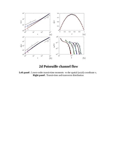
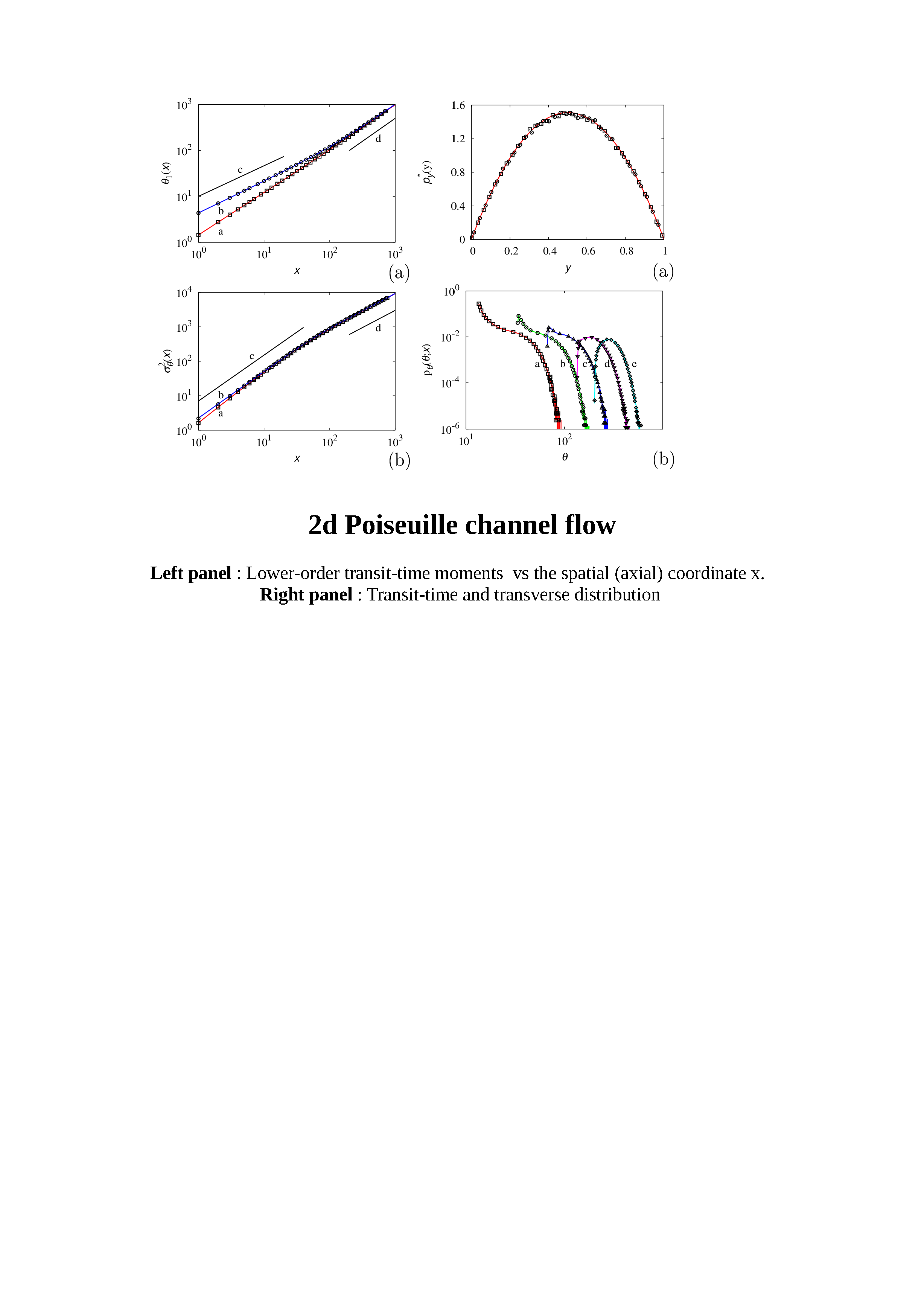
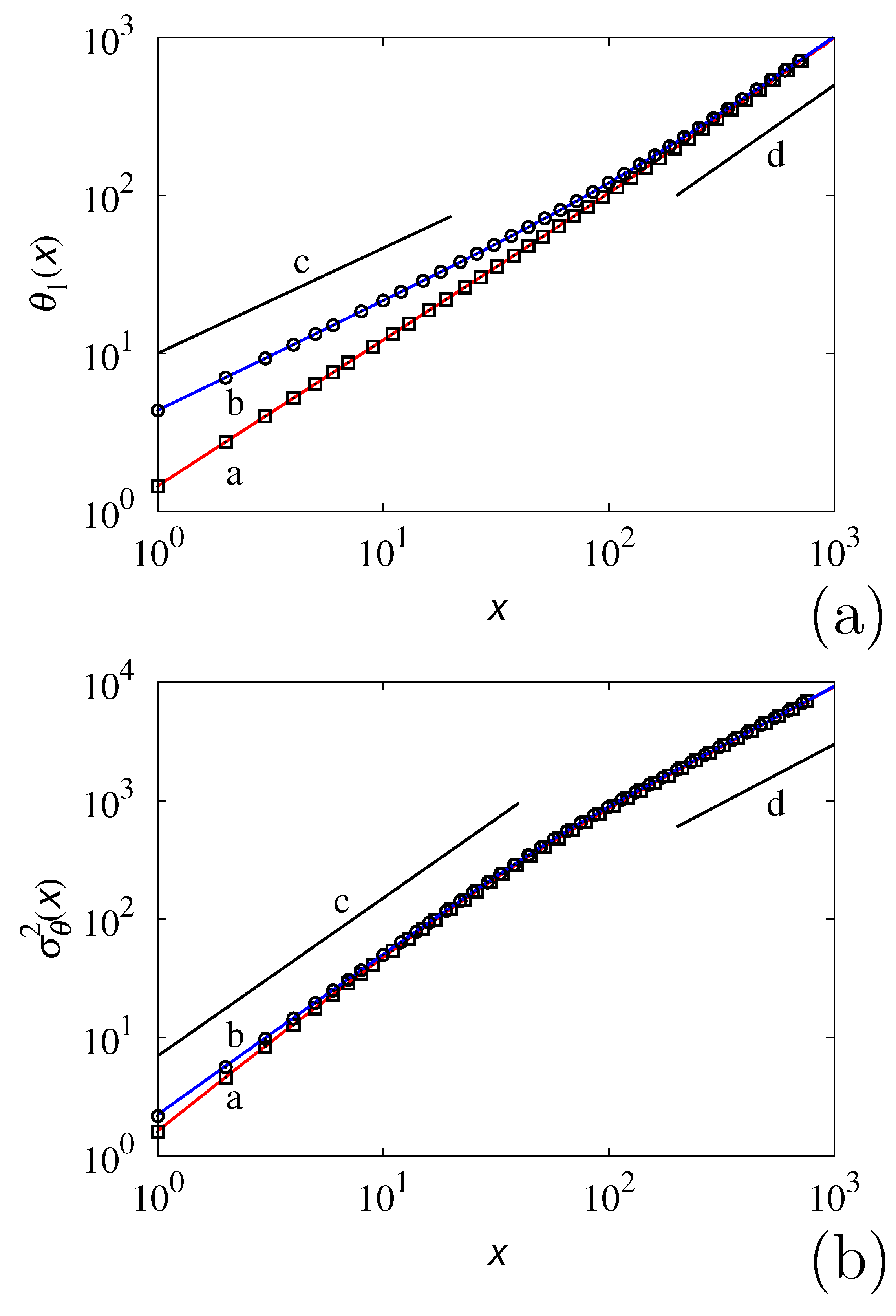
Conversely, the space-time inverse dynamics provides a direct framework to the first transit time process, as the temporal variable is parametrized with respect to x. Observe that the condition of positive subordination ensures that for each realization and for any value of x, there is one and only one transit time through the transversal cross section located at any value of x. Figure 4 and Figure 5 depict the comparison of the stochastic simulations of the statistics of transit times, by considering either the direct problem (i.e., Equation (8)), and the space-time inverse dynamics Equation (37). Figure 4 refers to the mean transit time ${\theta }_1\left(x\right)$ and to the second-order central moment ${\sigma }_{\theta }^2\left(x\right)={\theta }_2\left(x\right)-{\left({\theta }_1\left(x\right)\right)}^2$, starting from an ensemble of particles initially located at $x=0$. Two initial transverse distributions $p_{\mathrm{in},y}\left(y\right)$, $y\in [0,1]$, are considered in the simulations: (i) a uniform one, that is, $p_{\mathrm{in},y}\left(y\right)=1$, and (ii) and an impulsive one, where all the particles are initially located at $y=0$, $p_{\mathrm{in},y}\left(y\right)=\delta \left(y\right)$. Therefore, the initial condition for $p(x,y;t)$ is $p(x,y;0)=\delta \left(x\right)p_{\mathrm{in},y}\left(y\right)$. An ensemble of ${10}^6$ particles is used in the simulations. The comparison of the results deriving from the estimate of transit-time statistics from the direct equation and from the solution of the space-time inverse equation reveals the excellent matching between these two approaches.

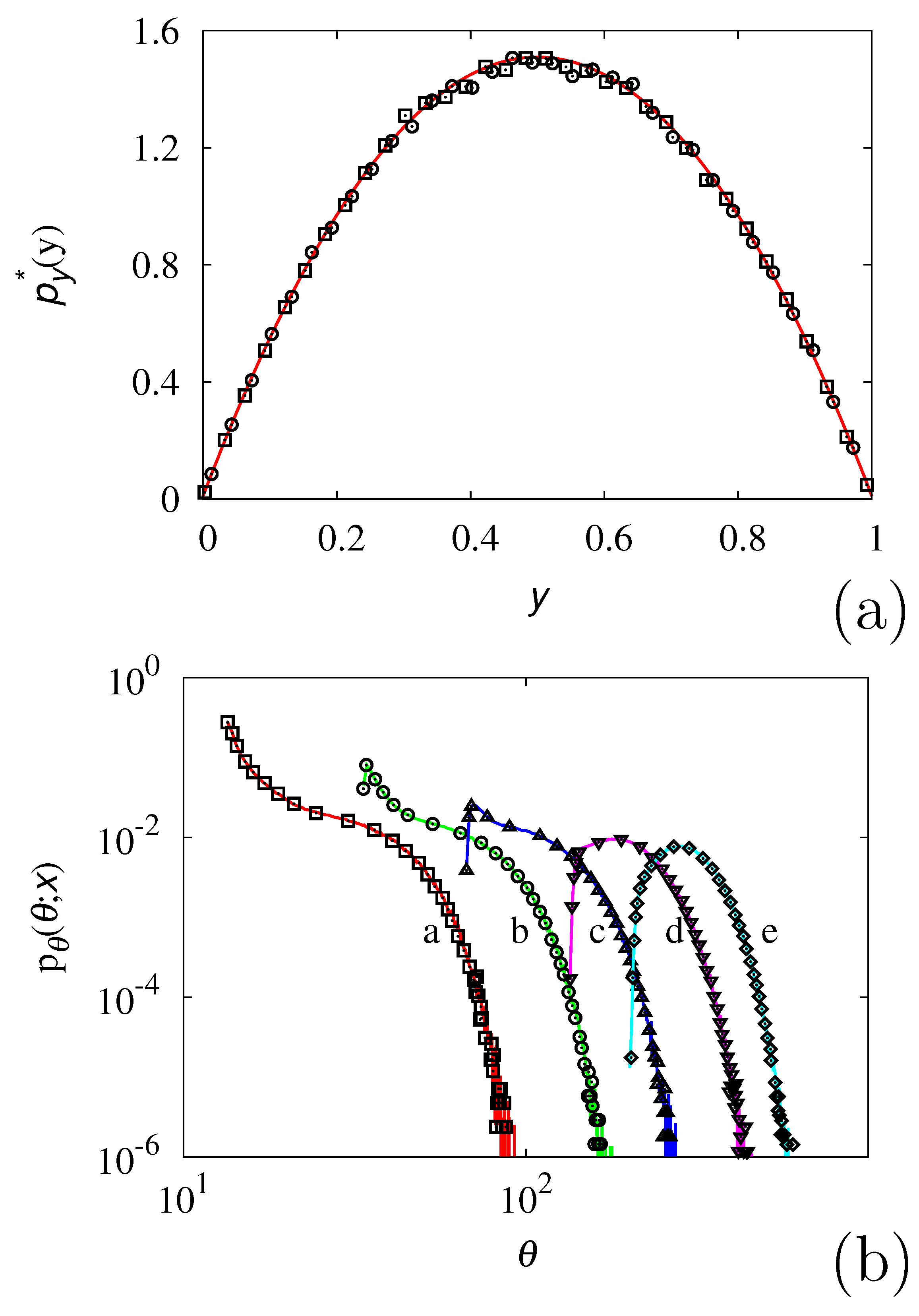
A similar comparison in terms of the transit-time probability density functions $p_{\theta }(\theta ,x)={\overline{p}}_t{(t;x)|}_{t=\theta }$ is depicted in Figure 5 panel (b) at several values of x, while panel (a) depicts the resulting stationary transversal distribution $p_y^{*}\left(y\right)={\overline{p}}^{*}\left(y\right)$ that, in the present case, is parabolic $p_y^{*}\left(y\right)=Av\left(y\right)$, where A is a normalization constant.

The space-time inversion process provides a way for establishing a direct connection between spatial and temporal moments in the analysis of particle dispersion in channel flows, and this issue will be developed in forthcoming works.

Stochastic thermodynamics—Consider a classical Ornstein-Uhlenbeck model for a particle of mass m in a conservative potential $\varphi \left(x\right)$ in the presence of stochastic fluctuations

$$\begin{array}{}\mathrm{(39)}& \hfill dx& =& v\left(t\right)dt\hfill \mathrm{(40)}& \hfill mdv\left(t\right)& =& -\eta v\left(t\right)dt-{\varphi }^{\prime }\left(x\left(t\right)\right)dt+\sqrt{2D}\eta dw\left(t\right),\hfill \end{array}$$

where $\eta$ is the friction factor. In stochastic thermodynamics [50] one is interested in the statistics of the dissipated heat $Q\left(t\right)$, and in the work $L_s\left(t\right)$ exerted by the stochastic fluctuations

$$dQ\left(t\right)=\eta v^2\left(t\right)dt,d{L}_s\left(t\right)=\sqrt{2D}\eta v\left(t\right)\circ dw\left(t\right),$$

(41)

where “○” indicates the Stratonovich approach to Stieltjes integrals in order to be consistent with the classical definition of the kinetic energy. In this case, space-time inversion can be applied to the dissipated heat, in order to obtain information on the statistics of the stochastic work $L_s$ and of the kinetic energy $m{v}^2/2$ at a prescribed value of the dissipation. In order to ensure positive subordination, the definition of the dissipated heat should be “mollified” by an arbitrarily small but positive factor $\epsilon >0$, as $dQ\left(t\right)=\left[\epsilon +\eta v^2\left(t\right)\right]dt$, and the limit for $\epsilon \to 0$ considered.

It is also clear that the entropy $S\left(t\right)$ could be used as a subordinated process in order to obtain a parametrization of the dynamics with respect to it instead of the physical time t. This approach could have interesting thermodynamics implications and will be addressed elsewhere.

Fractal time models—There is a straightforward application of the space-time inversion related to the idea by R. Hilfer of introducing transport models defined with respect to “a fractal time” [43,44]. To this purpose, consider a pure diffusion process defined by the Langevin model

$$dy\left(t\right)=\sqrt{2D}dw\left(t\right),$$

(42)

with $y\left(0\right)=0$. We are interested in transforming this model parametrized with respect to the physical time t, into a model parametrized with respect to some fractal time, that is itself a stochastic process. Since $y\left(t\right)\sim w\left(t\right)$, the simplest way to achieve this is to define $\tau$ as a positive subordination of $w\left(t\right)$, for example, as

$$d\tau \left(t\right)=\left[\epsilon +{\left|y\left(t\right)\right|}^{\nu }\right]dt,$$

(43)

where $\epsilon >0$ is a small quantity and $\nu >0$. The space-inversion of this process is analogous of the corresponding problem developed in the previous Section for the Poiseuille flow, and leads to a form of diffusion equation in the fractal time $\tau$, defined by the Langevin dynamics

$$dy\left(\tau \right)=\sqrt{\frac{2D}{\epsilon +{\left|y\left(\tau \right)\right|}^{\nu }}}d\overline{w}\left(\tau \right),$$

(44)

where $\overline{W}\left(\tau \right)$ is a Wiener process parametrized with respect to $\tau$, to be interpreted a la Ito.

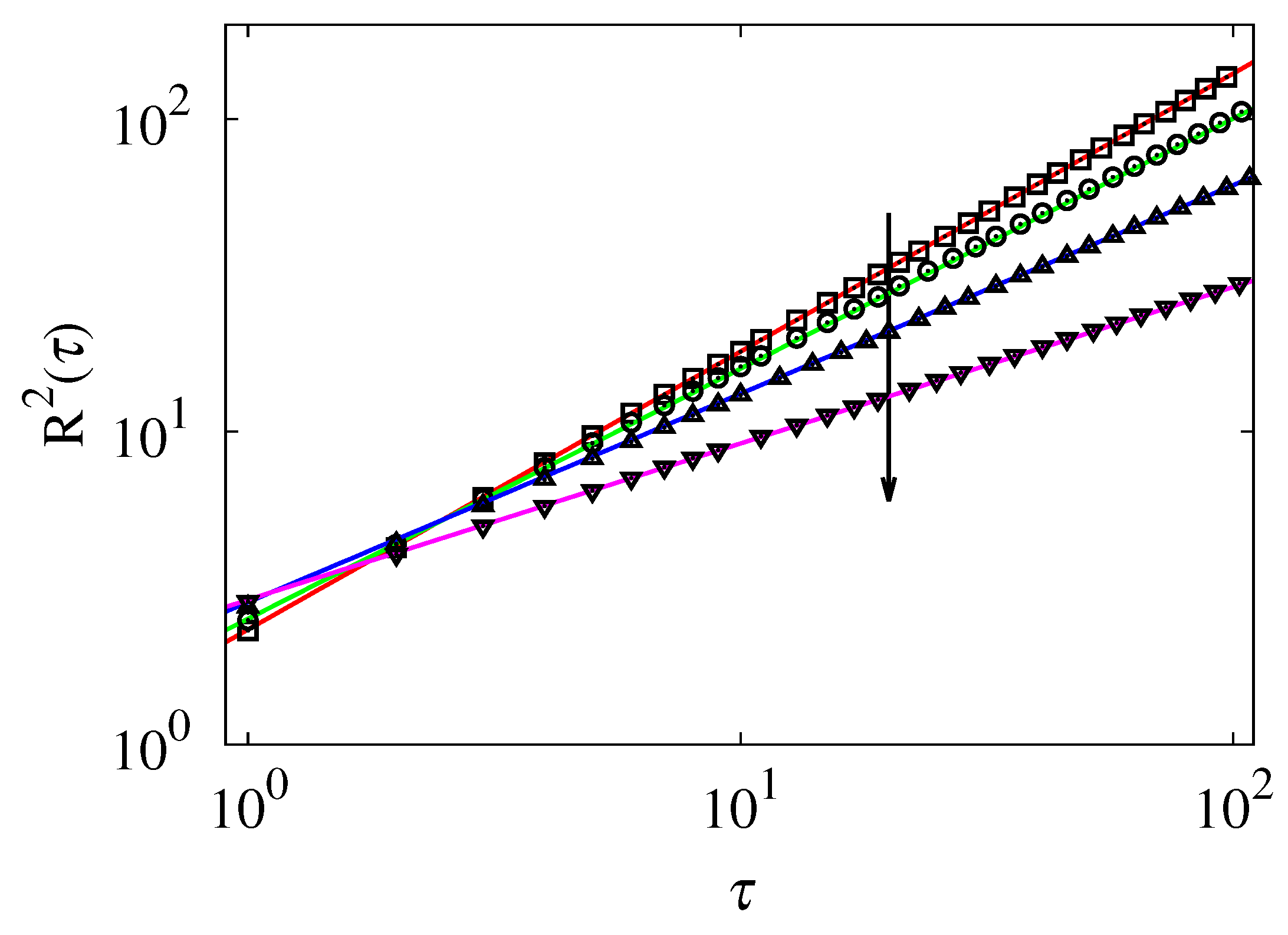
Figure 6 depicts the mean square displacement $R^2\left(\tau \right)=\langle y^2\left(\tau \right)\rangle$ vs the fractal time $\tau$ at $D=1$, $\epsilon ={10}^{-3}$, for different values of the exponent $\nu$. Simple scaling arguments indicate that $R^2\left(\tau \right)\sim {\tau }^{2/(2+\nu )}$ as observed in the stochastic simulations of the inverted process (44).

7. Concluding Remarks

This article has developed the setting of the space-time inversion problems and the use of mollified dynamics in order to resolve this problem, and obtain its correct statistical description via a Fokker-Planck equation. If the original (direct) dynamics is described by means of a nonlinear Langevin equation driven by Wiener fluctuations, the Fokker-Planck equation for the space-inverted process cannot be explained in terms of the existing models ($\lambda$-integrals) of stochastic calculus, while it can be derived by enforcing a mollified approach for example, using Poisson-Kac processes. In the limit of infinite propagation velocity, the corresponding Fokker-Planck equation can be interpreted as the statistical description of a Wiener-driven nonlinear Langevin equation defined in terms of mixed-order stochastic integrals.

It is important to point out the connections between the present theory and the discrete models of space-time transport developed in References [51,52]. The connections between the present theory and fluid dynamic applications (both as regards particle dispersion and fluid mixing) will be developed elsewhere.