Abstract
The newly constructed optimal perturbation iteration procedure with Laplace transform is applied to obtain the new approximate semi-analytical solutions of the fractional type of damped Burgers’ equation. The classical damped Burgers’ equation is remodeled to fractional differential form via the Atangana–Baleanu fractional derivatives described with the help of the Mittag–Leffler function. To display the efficiency of the proposed optimal perturbation iteration technique, an extended example is deeply analyzed.
1. Introduction
Partial differential equations obtained in many real-life problems modeled in terms of time or spatial variables need to be analyzed in order to understand the behaviors of the proposed models. These equations are mostly nonlinear partial differential equations, sometimes due to the basic structure of real-life problems and sometimes due to the complexity of the system, which often cannot be solved analytically by conventional methods. Therefore, by developing various solution techniques, existing methods have been improved and different solution methods have been presented.
During the last decade, some of the most remarkable methods developed to obtain the analytical, semi-analytical, and numerical solutions of partial differential equations are the optimal homotopy asymptotic method [1,2,3], homotopy analysis method [4], modified simple equation method [5], homotopy perturbation method [6,7], and optimal perturbation iteration method [8,9,10,11,12,13].
On the one hand, as partial derivatives, which are calculated by using different definitions of integral and derivative in fractional calculus, allow us to examine problems in more depth, numerical solutions of fractional partial differential equations have begun to be investigated in many articles. Following the Jafari’s Adomian Decomposition method study for fractional diffusion and wave equations in 2006 [14], the variational iteration method for the fractional Burgers’ equation [15,16], the homotopy perturbation method for fractional Kdv-Burgers’ equations and fractional Lotka–Volterra equations [7,17,18], homotopy analysis method for fractional damped Burgers’ and Chan–Allen equations [19] has been extended. Many authors working with fractional analysis have introduced many definitions of fractional integrals and derivatives, which try to eliminate the deficiencies in the computational process and facilitate a better understanding of the dynamics of real life problems. In some studies, local and non-local fractional integral and derivative definitions have been proposed in order to better define the dynamics of the problems. In 2016, Atangana and Baleanu introduced significant non-local Atangana–Baleanu fractional derivatives [20]. This definition has great advantage, especially when using Laplace transforms to solve some initial conditional physical problems. In the last three years, by taking this definition into account, better modeling and investigation of problems in different fields has been achieved successfully [21,22,23,24,25,26,27,28,29,30,31,32,33,34,35,36,37].
The classical damped Burgers’ equation can be given as [38]
In this current study, we will analyze the fractional form of the Equation (1) with the Atangana–Baleanu derivative. We try to find the new semi-analytical solutions of the fractional damped Burgers’ equation by optimal perturbation iteration technique. In the literature, the damped Burgers’ Equation (1) emerges as an exemplary equation for defining diffuse waves that are subject to diffusion in fluid mechanics, where is a constant parameter, which denotes the kinematics viscosity equals to Reynolds number and is a positive constant. Additionally, the equation which also appears as a model equation in gas dynamics, nonlinear acoustics has been studied for its numerical solutions in [19,24,38]. Malfliet has used tanh method as a perturbation technique to obtain approximate solution of the damped Burgers equation [39]. Yılmaz and Karasözen used COMSOL Multiphysics for dealing with optimal control problems for the unsteady Burgers equation [40].
By using the fractional differential operators instead of integer order derivatives, it is known that a memory effect occurs in any dynamical system. It means that the future state of a physical system depends not only on past data, but also on present data [22,23]. Therefore, it is reasonable to convert many differential equations to fractional differential equations to intensely analyze the solutions. The main reason why we use the definition of Atangana–Baleanu derivative is that this new Atangana–Baleanu operator overcomes the issues in the kernel structures found in the Caputo–Fabrizio derivative and also Caputo–Riemann–Liouville derivative [20].
Thus, let us introduce the fractional damped Burgers’ equation by replacing the time-dependent derivative in the damped Burgers’ equation given by Equation (1) equation with the newly defined ABC derivative:
In order to obtain the semi-analytical solutions to this new proposed model, we use a scheme including the optimal perturbation iteration technique and Laplace technique. The organization of the rest of the paper is as follows. In Section 2, we introduce the definition and the Laplace property of ABC fractional derivative for forming the base of our study. In Section 3, we propose a solution procedure to solve fractional damped Burgers’ equation via optimal perturbation iteration algorithms. Finally, in Section 4, the numerical examples are given in order to demonstrate our results.
2. Preliminaries and Definitions
Some basic definitions and the Laplace transform property of Atangana–Baleanu (AB) derivative that we considered are given in this part. For the further theory behind the new AB derivative, the reader may refer to work in [20].
Definition 1.
Let z and α be two complex numbers with . One parameter Mittag–Leffler function is defined by.
This special function is known as an entire function of z and the infinite series converges locally uniformly in the whole complex plane.
Definition 2.
Let and Ω be an open subset of real numbers. The Sobolev space is defined by
.
Definition 3.
For , let be the normalization function that satisfies the property and let . Combining with the Caputo derivative, the AB time-fractional derivative is defined by
Property 1.
By taking the Laplace transform of both sides of the new defined ABC fractional derivative Equation (3), we have
3. Analysis of Fractional Damped Burgers’ Equation via OPIM
Optimal perturbation iteration method (OPIM) is first developed by using the ideas of perturbation iteration [8,9] and optimal homotopy asymptotic methods [1,2,3]. It has been used for solving many different types of nonlinear differential equations [41,42,43,44,45,46]. In this section, we use OPIM and Laplace transform to obtain approximate solutions of the extended fractional damped Burgers’ equation.
Let us consider Equation (2) with the initial condition . Then, by applying the Laplace transform to Equation (2) as
The Equation (5) can be written as
The first term of the Equation (6) is the Laplace transform of fractional part and it can be computed as in Property 3. With the help of the definitions in the previous section, one can get
where
is the closed form of the nonlinear term of the main problem (2). Now, we exploit OPIM to decompose the nonlinear term. The following formulation can be used to summarize the technique.
(a) The perturbation parameter can be artificially embedded into Equation (8) as
For example, for our case, can be replaced into the Equation (8) as
(b) In order to construct the iteration scheme, we use the idea of classical perturbation theory [47]. The approximate solution may be taken in the perturbation expansion as
where is the correction term and . In order to handle the nonlinear term, one can use the Taylor series for multivariable functions. To achieve that, we first substitute the Equation (11) into Equation (10), then we expand the resulting closed form function in a Taylor series with only first derivatives. This will give the following algorithm,
where
It should be noted that one can use higher-order derivatives to establish algorithms. However, in that case, computations of the derivatives get harder and harder and one needs higher capacity computer programs.
Using Equation (7) and computing all derivatives, functions at gives
It should be emphasized that we use the decomposed form of the nonlinear term in the Laplace transform of the second term of the above equation. Equation (13) is an iteration procedure for OPIM algorithms of fractional damped Burgers’ Equation (2). We may start to iteration scheme by selecting the first initial function . This function has to satisfy the given initial conditions. can be calculated from the Equation (13) by using and so on.
(c) In order to increase the accuracy of the solutions and efficiency of the technique, we propose to follow the following equation,
where for are the parameters that control the convergence of approximate solutions. Performing the calculations for , one can get mth order approximate solutions as follows,
(d) Substituting the approximate solution into the Equation (2), the general problem is transformed to the following residual,
Undoubtedly, if residual (16) is identically zero, then the approximation is the desired analytical solution. However, such a case does not usually occur in fractional differential equations. On the other hand, the functional can be minimized as
where , and denote the domain of the physical equation. Optimum values of can be determined from the conditions
The constants may be obtained from
where . There are much more information about finding these parameters in the papers [1,3].
4. Numerical Example
In the present section, we solve the following fractional damped Burgers’ equation [38],
with the initial condition
for different values of and .
The Equation (20) can be rewritten as
where is the perturbation parameter. By taking the approximate solution as
and using the properties of Laplace transform, optimal perturbation iteration algorithm (OPIA) can be obtained. One can initiate the procedures by taking the Equation (21) as an initial function . The first correction term can be calculated as
In order to enhance the accuracy of the approximate solutions, we use the idea of convergence-control parameters. Proceeding as mentioned in Section 3, a parameter must be inserted into the the first correction term as
Then, the first-order approximate OPIM solution will be
By proceeding in a similar manner, one can have the following approximate OPIM solutions
and so on. In order to determine the unknown constants, the method of least squares or collocation techniques can be used as mentioned in Section 2. Before doing those calculations, we need to attain some values to the unknown parameters. For and using the collocation technique, unknown parameters are obtained as for the third-order approximate solutions. Inserting these constants into the obtained solutions, one can get the semi-analytical approximations for the fractional damped Burgers’ equation. Table 1 and Table 2 show the computed parameters for different values of and . The setting was randomly selected in order to show that the proposed technique is valid for any parameter combination.

Table 1.
Optimal perturbation iteration method (OPIM) constants for different values of α and λ for third-order solutions.
Table 2.
OPIM constants for different values of α and λ for fourth-order solutions.
Table 3 and Table 4 display the absolute residual error for third-order approximate OPIM solutions of the fractional damped Burgers’ equation for different ’s at some control points x. Furthermore, Figure 1, Figure 2, Figure 3, Figure 4, Figure 5 and Figure 6 display the different effects of the approximations for various values of ’s.
Table 3.
Absolute residual errors of the third-order OPIM solutions at x = 0.5.
Table 4.
Absolute residual errors of the third-order OPIM solutions at x = 0.75.
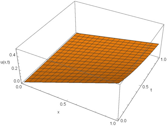
Figure 1.
Third-order OPIM approximate solution of the Equation (20) for α = 0.5, λ = 1.
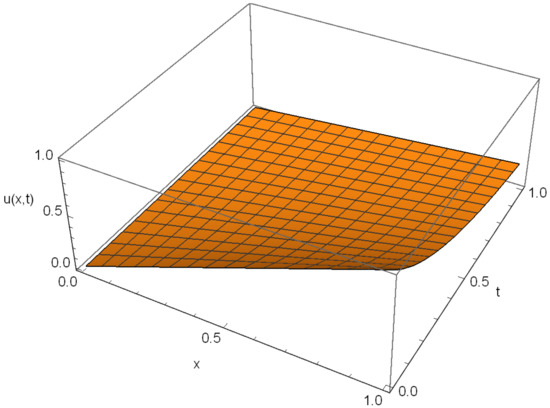
Figure 2.
Third-order OPIM approximate solution of Equation (20) for α = 1, λ = 1.
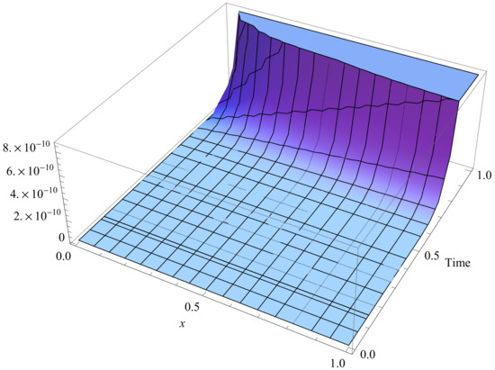
Figure 3.
Residual errors of fourth-order OPIM approximate solution of Equation (20) for α = 0.5, λ = 0.5.
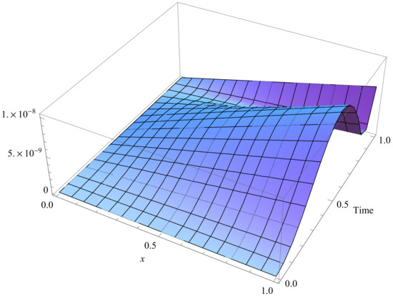
Figure 4.
Residual errors of fourth-order OPIM approximate solution of Equation (20) for α = 0.75, λ = 1.
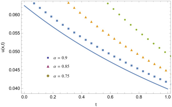
Figure 5.
Fourth-order OPIM approximate solution for distinct values of α at x = 0.25, λ = 0.5 with α = 1 (−).
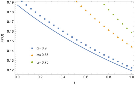
Figure 6.
Fourth-order OPIM approximate solution for distinct values of α at x = 0.75, λ = 0.75 with α = 1 (−).
This problem has been also considered in [19] by Esen et al. They use the homotopy analysis method (HAM) for solving the fractional damped Burgers’ equation. From Table 5, one can see the comparison of OPIM and HAM solutions for different values of parameters. We can say that both methods yield a very effective solution for this equation.
Table 5.
Comparison of absolute residual errors of the sixth-order OPIM and HAM solutions at x = 0.25 for α = 1.
It is clear that a symbolic computer program is needed to deal with high volume equations. We use Mathematica 11.0 to compute complex derivatives and iteration steps.
5. Conclusions
In this research, we first aim to reconstruct the damped Burgers’ equation with a new fractional operator. Then, optimal perturbation iteration technique has been implemented to get the approximate solutions of the extended version of the damped Burgers’ equation. While doing this, we use Laplace transform to reshape the equations for applying suitably OPIM algorithms to damped Burgers’ equations. We can say that the most important portion of the present study is modeling the damped Burgers’ equations with the definition of fractional derivative in the sense of ABC in
Section 1 and successfully implementing OPIM to that model in Section 3. Numerical results show that the suggested scheme is favorably applied to damped Burgers’ equations and also this means that this process can be generalized for solving linear–nonlinear partial fractional mathematical models in nature. It can be also deduced that the usage of fractional operators bring the new paradigms in the area of mathematics or engineering.
Author Contributions
S.D. contributed in conceptualization, investigation, methodology, validation and writing the original draft; A.K. contributed in conceptualization, investigation, methodology, validation and writing the original draft; M.D.l.S. contributed in funding acquisition, methodology, project administration, supervision, validation, visualization and editing. All authors agree and approve the final version of this manuscript.
Funding
This work was supported in part by the Basque Government, through project IT1207-19.
Acknowledgments
The authors thank the Basque Government for Grant IT1207-19. We would like to express our gratitude to the anonymous referees for their helpful suggestions and corrections.
Conflicts of Interest
The author declares no conflicts of interest.
References
- Marinca, V.; Herisanu, N. Application of optimal homotopy asymptotic method for solving nonlinear equations arising in heat transfer. Int. Commun. Heat Mass Transf. 2008, 35, 710–715. [Google Scholar] [CrossRef]
- Bildik, N.; Deniz, S. Comparative study between optimal homotopy asymptotic method and perturbation-iteration technique for different types of nonlinear equations. Iran. J. Sci. Technol. Trans. A Sci. 2018, 42, 647–654. [Google Scholar] [CrossRef]
- Iqbal, S.; Idrees, M.; Siddiqui, A.M.; Ansari, A.R. Some solutions of the linear and nonlinear Klein–Gordon equations using the optimal homotopy asymptotic method. Appl. Math. Comput. 2010, 216, 2898–2909. [Google Scholar] [CrossRef]
- Rashidi, M.M.; Domairry, G.; Dinarvand, S. Approximate solutions for the Burger and regularized long wave equations by means of the homotopy analysis method. Commun. Nonlinear Sci. Numer. Simul. 2009, 14, 708–717. [Google Scholar] [CrossRef]
- Khan, M.A.; Akbar, M.A.; Belgacem, F.B.M. Solitary wave solutions for the Boussinesq and Fisher equations by the modified simple equation method. Math. Lett. 2016, 2, 1–18. [Google Scholar]
- Saad, K.M.; Deniz, S.; Agarwal, P. Approximate solutions for a cubic autocatalytic reaction. Electron. J. Math. Anal. Appl. 2019, 7, 14–32. [Google Scholar]
- Kadem, A.; Baleanu, D. Homotopy perturbation method for the coupled fractional Lotka–Volterra equations. Rom. J. Phys. 2011, 56, 332–338. [Google Scholar]
- Deniz, S. Optimal perturbation iteration method for solving nonlinear heat transfer equations. J. Heat Transf. ASME 2017, 139, 074503-1. [Google Scholar] [CrossRef]
- Deniz, S.; Bildik, N. Applications of optimal perturbation iteration method for solving nonlinear differential equations. AIP Conf. Proc. 2017, 1798, 020046. [Google Scholar]
- Deniz, S.; Bildik, N. A new analytical technique for solving Lane-Emden type equations arising in astrophysics. Bull. Belg. Math. Soc. Simon Stevin 2017, 24, 305–320. [Google Scholar] [CrossRef]
- Bildik, N.; Deniz, S. New analytic approximate solutions to the generalized regularized long wave equations. Bull. Korean Math. Soc. 2018, 55, 749–762. [Google Scholar]
- Bildik, N.; Deniz, S. A practical method for analytical evaluation of approximate solutions of Fisher’s equations. ITM Web Conf. 2017, 13, 01001. [Google Scholar] [CrossRef]
- Bildik, N.; Deniz, S. Solving the Burgers’ and regularized long wave equations using the new perturbation iteration technique. Numer. Methods Partial Differ. Equ. 2018, 34, 1489–1501. [Google Scholar] [CrossRef]
- Jafari, H.; Daftardar-Gejji, V. Solving linear and nonlinear fractional diffusion and wave equations by Adomian decomposition. Appl. Math. Comput. 2006, 180, 488–497. [Google Scholar] [CrossRef]
- Wu, G.C.; Baleanu, D. Variational iteration method for the Burgers’ flow with fractional derivatives—New Lagrange multipliers. Appl. Math. Model. 2013, 37, 6183–6190. [Google Scholar] [CrossRef]
- Inc, M. The approximate and exact solutions of the space-and time-fractional Burgers equations with initial conditions by variational iteration method. J. Math. Anal. Appl. 2008, 345, 476–484. [Google Scholar] [CrossRef]
- Wang, Q. Homotopy perturbation method for fractional KdV-Burgers equation. Chaos Solitons Fractals 2008, 35, 843–850. [Google Scholar] [CrossRef]
- Sezer, S.A.; Yıldırım, A.; Mohyud-Din, S.T. He’s homotopy perturbation method for solving the fractional KdV-Burgers-Kuramoto equation. Int. J. Numer. Methods Heat Fluid Flow 2011, 21, 448–458. [Google Scholar] [CrossRef]
- Esen, A.; Yagmurlu, N.M.; Tasbozan, O. Approximate analytical solution to time-fractional damped Burger and Cahn-Allen equations. Appl. Math. Inf. Sci. 2013, 7, 1951. [Google Scholar] [CrossRef]
- Atangana, A.; Baleanu, D. New fractional derivatives with nonlocal and non-singular kernel: Theory and application to heat transfer model. arXiv 2016, arXiv:1602.03408. [Google Scholar] [CrossRef]
- Agarwal, P.; El-Sayed, A.A. Non-standard finite difference and Chebyshev collocation methods for solving fractional diffusion equation. Phys. A Stat. Mech. Appl. 2018, 500, 40–49. [Google Scholar] [CrossRef]
- Kumar, D.; Singh, J.; Baleanu, D. A new analysis for fractional model of regularized long-wave equation arising in ion acoustic plasma waves. Math. Methods Appl. Sci. 2017, 40, 5642–5653. [Google Scholar] [CrossRef]
- Kumar, D.; Singh, J.; Baleanu, D. Analysis of regularized long-wave equation associated with a new fractional operator with Mittag–Leffler type kernel. Phys. A Stat. Mech. Appl. 2018, 492, 155–167. [Google Scholar] [CrossRef]
- Singh, J.; Kumar, D.; Al Qurashi, M.; Baleanu, D. Analysis of a new fractional model for damped Bergers’ equation. Open Phys. 2017, 15, 35–41. [Google Scholar] [CrossRef]
- Bildik, N.; Deniz, S. A new fractional analysis on the polluted lakes system. Chaos Solitons Fractals 2019, 122, 17–24. [Google Scholar] [CrossRef]
- Atangana, A.; Koca, I. Chaos in a simple nonlinear system with Atangana–Baleanu derivatives with fractional order. Chaos Solitons Fractals 2016, 89, 447–454. [Google Scholar] [CrossRef]
- Alkahtani, B.S.T. Chua’s circuit model with Atangana–Baleanu derivative with fractional order. Chaos Solitons Fractals 2016, 89, 547–551. [Google Scholar] [CrossRef]
- Bildik, N.; Deniz, S.; Saad, K.M. A comparative study on solving fractional cubic isothermal auto–catalytic chemical system via new efficient technique. Chaos Solitons Fractals 2020, 132, 109555. [Google Scholar] [CrossRef]
- Algahtani, O.J.J. Comparing the Atangana–Baleanu and Caputo–Fabrizio derivative with fractional order: Allen Cahn model. Chaos Solitons Fractals 2016, 89, 552–559. [Google Scholar] [CrossRef]
- Koca, I.; Atangana, A. Solutions of Cattaneo-Hristov model of elastic heat diffusion with Caputo–Fabrizio and Atangana–Baleanu fractional derivatives. Therm. Sci. 2017, 21 Pt A, 2299–2305. [Google Scholar] [CrossRef]
- Gómez-Aguilar, J.F. Chaos in a nonlinear Bloch system with Atangana–Baleanu fractional derivatives. Numer. Methods Partial Differ. Equ. 2018, 34, 1716–1738. [Google Scholar] [CrossRef]
- Koca, I. Modelling the spread of Ebola virus with Atangana–Baleanu fractional operators. Eur. Phys. J. Plus 2018, 133, 100. [Google Scholar] [CrossRef]
- Yavuz, M.; Ozdemir, N.; Baskonus, H.M. Solutions of partial differential equations using the fractional operator involving Mittag–Leffler kernel. Eur. Phys. J. Plus 2018, 133, 215. [Google Scholar] [CrossRef]
- Saad, K.M.; Atangana, A.; Baleanu, D. New fractional derivatives with non-singular kernel applied to the Burgers equation. Chaos Interdiscip. J. Nonlinear Sci. 2018, 28, 063109. [Google Scholar] [CrossRef] [PubMed]
- Atangana, A.; Gómez-Aguilar, J.F. Numerical approximation of Riemann-Liouville definition of fractional derivative: From Riemann-Liouville to Atangana-Baleanu. Numer. Methods Partial Differ. Equ. 2018, 34, 1502–1523. [Google Scholar] [CrossRef]
- Sheikh, N.A.; Ali, F.; Khan, I.; Gohar, M.; Saqib, M. On the applications of nanofluids to enhance the performance of solar collectors: A comparative analysis of Atangana–Baleanu and Caputo–Fabrizio fractional models. Eur. Phys. J. Plus 2017, 132, 540. [Google Scholar] [CrossRef]
- Toufik, M.; Atangana, A. New numerical approximation of fractional derivative with non-local and non-singular kernel: Application to chaotic models. Eur. Phys. J. Plus 2017, 132, 444. [Google Scholar] [CrossRef]
- Vaganan, B.M.; Kumaran, M.S. Kummer function solutions of damped Burgers equations with time-dependent viscosity by exact linearization. Nonlinear Anal. Real World Appl. 2008, 9, 2222–2233. [Google Scholar] [CrossRef]
- Malfliet, W. Approximate solution of the damped Burgers equation. J. Phys. A Math. Gen. 1993, 26, L723. [Google Scholar] [CrossRef]
- Yılmaz, F.; Karasözen, B. Solving optimal control problems for the unsteady Burgers equation in COMSOL Multiphysics. J. Comput. Appl. Math. 2011, 235, 4839–4850. [Google Scholar] [CrossRef]
- Deniz, S.; Bildik, N. Optimal perturbation iteration method for Bratu–type problems. J. King Saud Univ. Sci. 2018, 30, 91–99. [Google Scholar] [CrossRef]
- Deniz, S. Semi-analytical investigation of modified Boussinesq-Burger equations. J. Balıkesir Univ. Inst. Sci. Technol. 2020, 22, 327–333. [Google Scholar]
- Deniz, S. Modification of coupled Drinfel’d-Sokolov-Wilson Equation and approximate solutions by optimal perturbation iteration method. Afyon Kocatepe Univ. J. Sci. Eng. 2020, 20, 35–40. [Google Scholar]
- Bildik, N.; Deniz, S. A new efficient method for solving delay differential equations and a comparison with other methods. Eur. Phys. J. Plus 2017, 132, 51. [Google Scholar] [CrossRef]
- Bildik, N.; Deniz, S. New approximate solutions to the nonlinear Klein-Gordon equations using perturbation iteration techniques. Discret. Contin. Dyn. Syst. S 2020, 13, 503. [Google Scholar] [CrossRef]
- Agarwal, P.; Deniz, S.; Jain, S.; Alderremy, A.A.; Aly, S. A new analysis of a partial differential equation arising in biology and population genetics via semi analytical techniques. Phys. A Stat. Mech. Appl. 2020, 542, 122769. [Google Scholar] [CrossRef]
- Nayfeh, A.H. Perturbation Methods; John Wiley & Sons: New York, NY, USA, 2008. [Google Scholar]
© 2020 by the authors. Licensee MDPI, Basel, Switzerland. This article is an open access article distributed under the terms and conditions of the Creative Commons Attribution (CC BY) license (http://creativecommons.org/licenses/by/4.0/).