Article

Discrete-Time Stochastic Quaternion-Valued Neural Networks with Time Delays: An Asymptotic Stability Analysis

by
Ramalingam Sriraman
1,
Grienggrai Rajchakit
2,*,
Chee Peng Lim
3,
Pharunyou Chanthorn
4 and
Rajendran Samidurai
5
1
Department of Science and Humanities, Vel Tech High Tech Dr. Rangarajan Dr. Sakunthala Engineering College, Avadi, Tamil Nadu-600 062, India
2
Department of Mathematics, Faculty of Science, Maejo University, Chiang Mai 50290, Thailand
3
Institute for Intelligent Systems Research and Innovation, Deakin University, Waurn Ponds VIC 3216, Australia
4
Research Center in Mathematics and Applied Mathematics, Department of Mathematics, Faculty of Science, Chiang Mai University, Chiang Mai 50200, Thailand
5
Department of Mathematics, Thiruvalluvar University, Vellore, Tamil Nadu-632115, India
*
Author to whom correspondence should be addressed.
Symmetry 2020, 12(6), 936; https://doi.org/10.3390/sym12060936
Submission received: 17 May 2020 / Revised: 26 May 2020 / Accepted: 29 May 2020 / Published: 3 June 2020

Abstract

:
Stochastic disturbances often cause undesirable characteristics in real-world system modeling. As a result, investigations on stochastic disturbances in neural network (NN) modeling are important. In this study, stochastic disturbances are considered for the formulation of a new class of NN models; i.e., the discrete-time stochastic quaternion-valued neural networks (DSQVNNs). In addition, the mean-square asymptotic stability issue in DSQVNNs is studied. Firstly, we decompose the original DSQVNN model into four real-valued models using the real-imaginary separation method, in order to avoid difficulties caused by non-commutative quaternion multiplication. Secondly, some new sufficient conditions for the mean-square asymptotic stability criterion with respect to the considered DSQVNN model are obtained via the linear matrix inequality (LMI) approach, based on the Lyapunov functional and stochastic analysis. Finally, examples are presented to ascertain the usefulness of the obtained theoretical results.

1. Introduction

The research on dynamical behavior analysis for NN models has attracted increasing attention in recent years and their results have been widely used in a variety of science and engineering disciplines [1,2,3,4,5,6,7,8,9]. The stability analysis of NN models is fundamental and important in the applications of NNs, which have received significant attention recently [3,4,5,6,7,8,9,10,11,12,13,14,15,16,17,18,19,20,21,22,23,24,25,26,27,28,29,30,31,32,33,34,35,36,37,38,39,40,41,42,43,44,45,46,47,48,49,50].
Indeed, most of the NN analyses are dealt with in the continuous-time case. Nevertheless, in today’s digital world, nearly all signals are digitalized for computer processing needs before and after transmission. In this regard, instead of continuous-time analysis, it is important to study discrete-time signals in implementing NN models. As a result, several researchers have studied various dynamical behaviors of discrete-time NN models. For example, a number of scientific results for various dynamic behaviors in the discrete-time case for both the real-world neural network (RVNN) as well as for the complex-valued neural network (CVNN) models have been published recently [6,7,8,9,10,11,12,13,21,22,23,24,25]. However, the corresponding research on the quaternion field is still in its infancy.
The characteristics of NN models, including RVNNs and CVNNs, can be analyzed based on their functional and/or structural properties. Recently, RVNNs have been commonly used in a number of engineering domains, such as optimization, associative memory, and image and signal processing [2,3,4,5,6,7,8,9,10,11,12]. However, with respect to 2 D affine transformations and XOR problems, RVNNs perform poorly. In view of this, complex properties are incorporated into RVNNs, leading to CVNNs [51,52,53] that can effectively address the 2 D affine transformation challenge and XOR problems. As a result, various CVNN-related models have received substantial research attention in both mathematical and practical analyses [25,26,27,28,29,30,31,32,33,34,35,36,37,38,39,40,41,42,43,44,45,46,47,48,49,50,51,52]. For instance, in [14,15,16,17], the problem of global stability, finite-time stability, and global Lagrange stability for continuous-time CVNNs were investigated using the Lyapunov stability theory. In [20,21,22,23,24,25], the investigations on discrete-time CVNNs and their corresponding sufficient conditions were discussed. Nevertheless, CVNN models are inefficient in handling higher dimension transformations, including color night vision, color image compression, and 3 D and 4 D problems [23,24,25].
On the other hand, the quaternion-valued signals and quaternion functions are very useful in the many engineering domains, such as in 3 D wind forecasting, polarized signal classification, and color night vision [54,55,56,57,58,59,60]. Undoubtedly, quaternion-based networks perform as good mathematical models to undertake these applications, due to the quaternion features. In view of this, quaternion-valued neural networks (QVNNs) have been developed by implementing quaternion algebra into CVNNs, in order to generalize RVNN and CVNN models with quaternion-valued activation functions, connection weights, and signal states [27,28,29,30,31,32,33,34,35,36,37,38,39,40,41,42,43,44,45,46,47,48,49,50,51,52,53,54,55]. The main advantage of a QVNN model is its capability of reducing the computational complexity in higher-dimensional problems. Therefore, the investigation of QVNN model dynamics is essential and important. Recently, many computational approaches for various QVNN models and their learning algorithms have been studied; e.g., exponential input-to-state stability, global Mittag–Leffler stability, synchronization analysis, global μ stability, global synchronization, and global asymptotic stability [26,27,28,29,30,31,32] have been studied for the continuous-time QVNNs. Very recently, the issue of mean-square exponential input-to-state stability for continuous-time stochastic memristive QVNNs with time-varying delays has been studied in [50]. Similarly, some other stability conditions have been defined for QVNN models [29,30,33,34,35,36]. In the earlier studies [37,38,39], the problems of global asymptotic stability, exponential stability, and exponentially periodicity, respectively, for discrete-time QVNNs, have been investigated with linear threshold activation functions.
In addition, the stochastic effects are unavoidable in most practical NN models. As a result, it is important to investigate stochastic NN models comprehensively, since their behaviors are susceptible by certain stochastic inputs. In practice, a stochastic neural network (SNN) is useful for the modeling of real-world systems, especially in the presence of external disturbances [41,42,43,44,45,46,47,48,49,50,51,52,53,54,55,56,57,58,59,60]. As a result, several aspects of SNN models have been analysed extensively in both continuous and discrete-time cases; e.g., the problems of passivity [40], robust stability [41], exponential stability [42], robust dissipativity [44], mean-square exponential input-to-state stability [49], and mean-square exponential input-to-state stability for QVNNs [50]. Other SNN-related dynamics have also been investigated in [43,45,46,47,48]. Nonetheless, studies on the dynamics of discrete-time QVNN (DSQVNN) models are limited. Indeed, the investigation on DSQVNN models with time delays and their mean-square asymptotic stability analysis is novel, which constitutes the main contribution of our paper.
Inspired by the above debate, our main aim is to do research into the sufficient conditions of DSQVNN models pertaining to their mean-square asymptotic stability. The designed DSQVNNs encompasses discrete-time stochastic CVNN and discrete-time stochastic RVNN as its special cases. Firstly, we equivalently represent a QVNN with four RVNNs via the real-imaginary separate type activation function. Secondly, we establish new linear matrix inequality (LMI)-based, sufficient conditions for the mean-square asymptotic stability of DSQVNNs via suitable Lyapunov functional and stochastic concepts. Note that several known results can be viewed as special cases of the results of our work. Finally, we provide numerical examples to illustrate the usefulness of the proposed results.
This study presents three key contributions. (1) This is the first analysis of the mean-square asymptotic stability of the considered DSQVNN models. (2) Unlike the traditional stability analysis, we establish new mean-square asymptotic stability criteria for the considered DSQVNN models, which is achieved through the Lyapunov functional and real-imaginary separate-type activation functions. (3) Developed sufficient conditions can be directly solved by the standard Matlab LMI toolbox. (4) The results of this study are more general and powerful than those in the existing discrete-time QVNN models in the literature.
In Section 2, we define the proposed problem model formally. We explain the new stability criterion in Section 3. The numerical examples are given in Section 4. Concluding remarks are given in the last section.

2. Mathematical Fundamentals and Definition of the Problem

2.1. Notations

We use R , C , and H to indicate the real, complex, and skew quaternion fields, respectively. The m × m matrices with entries from R , C , and H are denoted as R m × m , C m × m , and H m × m , while the m-dimension vectors are denoted as R m , C m , and H m , respectively. For any matrix Q and its transpose, the conjugate transposes are denoted as Q T and Q , respectively. In addition, a block diagonal matrix is denoted as d i a g { } , while the smallest and largest eigenvalues of Q are denoted as λ m i n ( Q ) and λ m a x ( Q ) , respectively. The Euclidean norm of a vector x and the mathematical expectation of a stochastic variable x are represented by x and E { x } , respectively. Meanwhile, given integers a, b with a < b , the discrete interval given by N [ a , b ] = { a , a + 1 , , b 1 , b } is denoted by N [ a , b ] , while the set of all functions ϕ : N [ ς , 0 ] H m is denoted by C ( N [ ς , 0 ] , H m ) , respectively. Moreover, we assume that ( Ω , F , P ) be a complete probability space with a filtration { F } t 0 satisfying the usual conditions. In a given matrix, a term induced by symmetry is denoted by □ in the matrix.

2.2. Quaternion Algebra

Firstly, we address the quaternion and its operating rules. The quaternion is expressed in the form:
x = x R + i x I + j x J + k x K H ,
where the real constants are denoted by x R , x I , x J , x K R , while the fundamental quaternion units are denoted by i, j, and k. The following Hamilton rules are satisfied:
i 2 = j 2 = k 2 = i j k = 1 , i j = j i = k ; j k = k j = i ; k i = i k = j .
which implies that quaternion multiplication has the non-commutativity property.
The following expressions define the operations between quaternions x = x R + i x I + j x J + k x K and y = y R + i y I + j y J + k y K . Note that the definitions of addition and subtraction of complex numbers are applicable to those of the quaternions as well.
(i)
Addition:
x + y = ( x R + y R ) + i ( x I + y I ) + j ( x J + y J ) + k ( x K + y K ) .
(ii)
Subtraction:
x y = ( x R y R ) + i ( x I y I ) + j ( x J y J ) + k ( x K y K ) .
The multiplication of x and y, which is in line with the Hamilton multiplication rules (1), is defined as follows:
(iii)
Multiplication:
x y = x R y R x I y I x J y J x K y K + i x R y I + x I y R + x J y K x K y J + j x R y J + x J y R x I y K + x K y I + k x R y K + x K y R + x I y J x J y I .
The following expression of | x | represents the module of a quaternion x = x R + i x I + j x J + k x K H :
| x | = x x = ( x R ) 2 + ( x I ) 2 + ( x J ) 2 + ( x K ) 2 ,
where the conjugate transpose of x is denoted by x = x R i x I j x J k x K . The following expression represents the norm of x: x = p = 1 m ( x R ) 2 + p = 1 m ( x I ) 2 + p = 1 m ( x J ) 2 + p = 1 m ( x K ) 2 .

2.3. Problem Definition

The DSQVNN model with time delays is considered; i.e.,
x p ( k + 1 ) = d p x p ( k ) + q = 1 m a p q g q ( x q ( k ς ) ) + u p ,
where p = 1 , , m , k N .
The model in (2) can be expressed in an equivalent vector form of
x ( k + 1 ) = D x ( k ) + A g ( x ( k ς ) ) + U ,
where the state variable and quaternion-valued neuron activation function are denoted by x ( k ) = [ x 1 ( k ) , , x m ( k ) ] T H and g ( x ( k ) ) = [ g 1 ( x 1 ( k ) ) , , g m ( x m ( k ) ) ] T H , respectively. In addition, U = [ u 1 , , u m ] T H the input vector. A self-feedback connection weight matrix with 0 d i < 1 is denoted by D = d i a g { d 1 , , d m } R m . Besides that, a connection weight matrix is denoted by A = ( a p q ) m × m H m × m , while the transmission delay is denoted by a positive scalar of ς .
Given the model in (3), its initial condition is
x ( k ) = ϕ ( k ) , k N [ ς , 0 ] ,
where ϕ ( k ) = [ ϕ 1 ( k ) , , ϕ m ( k ) ] T C ( N [ ς , 0 ] , H m ) .
Definition 1.
A vector x = [ x 1 , , x m ] T is said to be an equilibrium point of NN model (3), if it satisfies
x = D x + A g ( x ) + U .
Now, consider Ω = { ϕ | ϕ C ( N [ ς , 0 ] , H m ) } , which is similar to [20,21,22]. We can define the following, given ϕ Ω ,
| ϕ | = sup s N [ ς , 0 ] ϕ ( s ) ,
As such, Ω is a Banach space having uniform convergence in its topology. Suppose the solutions of the model in (3) are x ( k , ϕ ) and x ( k , ψ ) starting from ϕ and ψ , respectively, in which any ϕ , ψ Ω . As such, following the model in (3), we have
x ( k + 1 , ϕ ) x ( k + 1 , ψ ) = D ( x ( k , ϕ ) x ( k , ψ ) ) + A ( g ( x ( k ς , ϕ ) ) g ( x ( k ς , ψ ) ) ) .
Let y ( k + 1 ) = x ( k + 1 , ϕ ) x ( k + 1 , ψ ) , y ( k ) = x ( k , ϕ ) x ( k , ψ ) , f ( y ( k ς ) ) = g ( x ( k ς , ϕ ) ) g ( x ( k ς , ψ ) ) ) .
As a results, we can express (6) as
y ( k + 1 ) = D y ( k ) + A f ( y ( k ς ) ) .
A1: For y = y R + i y I + j y J + k y K H , y R , y I , y J , y K R , we can divide f q ( y ) into two parts, real and imaginary, as follows:
f q ( y ) = f q R ( y R ) + i f q I ( y I ) + j f q J ( y J ) + k f q K ( y K ) , q = 1 , , m ,
where f q R ( · ) , f q I ( · ) , f q J ( · ) , f q K ( · ) : R R . There exist constants ξ q R , ξ q R + , ξ q I , ξ q I + , ξ q J , ξ q J + , ξ q K , ξ q K + , such that for any α , β R and α β ,
ξ q R f q R ( α ) f q R ( β ) α β ξ q R + , ξ q I f q I ( α ) f q I ( β ) α β ξ q I + , ξ q J f q J ( α ) f q J ( β ) α β ξ q J + , ξ q K f q K ( α ) f q K ( β ) α β ξ q K + , q = 1 , , m ,
Denote
Ξ 1 R = d i a g ξ 1 R + ξ 1 R , , ξ m R + ξ m R , Ξ 2 R = d i a g ξ 1 R + + ξ 1 R 2 , , ξ m R + + ξ m R 2 , Ξ 1 I = d i a g ξ 1 I + ξ 1 I , , ξ m I + ξ m I , Ξ 2 I = d i a g ξ 1 I + + ξ 1 I 2 , , ξ m I + + ξ m I 2 , Ξ 1 J = d i a g ξ 1 J + ξ 1 J , , ξ m J + ξ m J , Ξ 2 J = d i a g ξ 1 J + + ξ 1 J 2 , , ξ m J + + ξ m J 2 , Ξ 1 K = d i a g ξ 1 K + ξ 1 K , , ξ m K + ξ m K , Ξ 2 K = d i a g ξ 1 K + + ξ 1 K 2 , , ξ m K + + ξ m K 2 .
In practical application of NN models, stochastic disturbances usually affect their performances. As such, stochastic disturbances must be included when studying the issue of network stability, which represent more realistic dynamic behaviors. Therefore, the following DSQVNN model is formulated:
y ( k + 1 ) = D y ( k ) + A f ( y ( k ς ) ) + σ ( k , y ( k ) ) w ( k ) .
Note that σ : R × H m H m × m is a noise intensity function, while w ( k ) is a scalar Wiener process (Brownian motion), which is defined on ( Ω , F , P ) with E [ w ( k ) ] = 0 , E [ w 2 ( k ) ] = 1 , E { w ( u ) w ( v ) } = 0 , ( u v ) .
For further analysis, we divide the NN model in (8) into both real and imaginary parts through the use of the quaternion multiplication. As such, we have
y R ( k + 1 ) = D y R ( k ) + A R f R ( y R ( k ς ) ) A I f I ( y I ( k ς ) ) A J f J ( y J ( k ς ) ) A K f K ( y K ( k ς ) ) + σ R ( k , y R ( k ) ) w ( k ) , y I ( k + 1 ) = D y I ( k ) + A R f I ( y I ( k ς ) ) + A I f R ( y R ( k ς ) ) + A J f K ( y K ( k ς ) ) A K f J ( y J ( k ς ) ) + σ I ( k , y I ( k ) ) w ( k ) , y J ( k + 1 ) = D y J ( k ) + A R f J ( y J ( k ς ) ) + A J f R ( y R ( k ς ) ) + A K f I ( y I ( k ς ) ) A I f K ( y K ( k ς ) ) + σ J ( k , y J ( k ) ) w ( k ) , y K ( k + 1 ) = D y K ( k ) + A R f K ( y K ( k ς ) ) + A K f R ( y R ( k ς ) ) + A I f J ( y J ( k ς ) ) A J f I ( y I ( k ς ) ) + σ K ( k , y K ( k ) ) w ( k ) ,
where
σ R ( k , y R ( k ) ) = R e ( σ ( k , y ( k ) ) , σ I ( k , y I ( k ) ) = I m ( σ ( k , y ( k ) ) , σ J ( k , y J ( k ) ) = I m ( σ ( k , y ( k ) ) , σ K ( k , y K ( t ) ) = I m ( σ ( k , y ( k ) ) .
The following expression denotes the initial condition of the model in (9):
y R ( k ) = ϕ R ( k ) , y I ( k ) = ϕ I ( k ) , y J ( k ) = ϕ J ( k ) , y K ( k ) = ϕ K ( k ) ,
for k N [ ς , 0 ] , where ϕ R ( k ) = R e ( ϕ ( k ) ) , ϕ I ( k ) = I m ( ϕ ( k ) ) , ϕ J ( k ) = I m ( ϕ ( k ) ) , ϕ K = I m ( ϕ ( k ) ) .
We denote A R = ( a p q R ) m × m R m × m , A I = ( a p q I ) m × m R m × m , A J = ( a p q J ) m × m R m × m , A K = ( a p q K ) m × m R m × m , f R ( y R ( k ς ) ) = [ f 1 R ( y 1 R ( k ς ) ) , , f m R ( y m R ( k ς ) ) ] T R m , f I ( y I ( k ς ) ) = [ f 1 I ( y 1 I ( k ς ) ) , , f m I ( y m I ( k ς ) ) ] T R m , f J ( y J ( k ς ) ) = [ f 1 J ( y 1 J ( k ς ) ) , , f m J ( y m J ( k ς ) ) ] T R m , f K ( y K ( k ς ) ) = [ f 1 K ( y 1 K ( k ς ) ) , , f m K ( y m K ( k ς ) ) ] T R m , σ R ( k ) = σ R ( k , y R ( k ) ) : R × R m R m × m , σ I ( k ) = σ I ( k , y I ( k ) ) : R × R m R m × m , σ J ( k ) = σ J ( k , y J ( k ) ) : R × R m R m × m , σ K ( k ) = σ K ( k , y K ( k ) ) : R × R m R m × m .
Denote
y ¯ ( t ) = [ ( y R ( k ) ) T , ( y I ( k ) ) T , ( y J ( k ) ) T , ( y K ( k ) ) T ] T , f ¯ ( y ¯ ( k ς ) ) = [ ( f R ( y R ( k ς ) ) ) T , ( f I ( y I ( k ς ) ) ) T , ( f J ( y J ( k ς ) ) ) T , ( f K ( y K ( k ς ) ) ) T ] T , σ ¯ ( k ) = [ ( σ R ( k ) ) T , ( σ I ( k ) ) T , ( σ J ( k ) ) T , ( σ K ( k ) ) T ] T , D ¯ = d i a g { D , D , D , D } , A ¯ = A R A I A J A K A I A R A K A J A J A K A R A I A K A J A I A R .
Therefore, the following expression can be used to represent the model in (9)
y ¯ ( k + 1 ) = D ¯ y ¯ ( k ) + A ¯ f ¯ ( y ¯ ( k ς ) ) + σ ¯ ( k ) w ( k ) .
Note that the following expression constitutes the initial condition of the model in (11)
y ¯ ( k ) = φ ( k ) , k N [ ς , 0 ] ,
where φ ( k ) = [ ϕ R ( k ) , ϕ I ( k ) , ϕ J ( k ) , ϕ K ( k ) ] T , with ϕ R ( s ) = sup ς s 0 | ϕ R ( s ) | , ϕ I ( s ) = sup ς s 0 | ϕ I ( s ) | ,
ϕ J ( s ) = sup ς s 0 | ϕ J ( s ) | , ϕ K ( s ) = sup ς s 0 | ϕ K ( s ) | .
A2: The noise intensity function σ s ( k , y s ( k ) ) , ( s = R , I , J , K ) with σ s ( k , 0 ) = 0 , it is able to satisfy the following conditions
( σ R ( k , y R ( k ) ) ) T σ R ( k , y R ( k ) ) ρ 1 ( y R ( k ) ) T y R ( k ) ( σ I ( k , y I ( k ) ) ) T σ I ( k , y I ( k ) ) ρ 2 ( y I ( k ) ) T y I ( k ) ( σ J ( k , y J ( k ) ) ) T σ J ( k , y J ( k ) ) ρ 3 ( y J ( k ) ) T y J ( k ) ( σ K ( k , y K ( k ) ) ) T σ K ( k , y K ( k ) ) ρ 4 ( y K ( k ) ) T y K ( k ) ,
where the positive constants are denoted by ρ 1 , ρ 2 , ρ 3 and ρ 4 .
Definition 2.
For any solution of the NN model in (8), it is asymptotically stable in the mean square sense if the following expression is true:
lim k E { y ( k ) 2 } = 0 .
Lemma 1.
[43] Given matrix 0 < W = W T R m × m , integers τ 1 and τ 2 satisfying τ 1 < τ 2 , and vector function y : N [ τ 1 , τ 2 ] R , in a way whereby the sums concerned are well-defined, we have
( τ 2 τ 1 + 1 ) u = τ 1 τ 2 y T ( u ) W y ( u ) u = τ 1 τ 2 y T ( u ) W u = τ 1 τ 2 y T ( u ) .

3. Main Results

Given the NN model in (11), we derive the new sufficient conditions to ensure its mean-square asymptotic stability.
Theorem 1.
The activation function can be separated into both real and imaginary parts based on assumption ( A 1 ) . Given the existence of matrices 0 < P a , ( a = 1 , 2 , 3 , 4 ) , 0 < Q b , ( b = 1 , 2 , 3 , 4 ) , 0 < R c , ( c = 1 , 2 , 3 , 4 ) , diagonal matrices 0 < L d , ( d = 1 , 2 , 3 , 4 ) , and scalars 0 < λ e , ( e = 1 , 2 , 3 , 4 ) the NN model in (11) is asymptotically stable in the mean square sense, subject to satisfying the following LMI:
P 1 < λ 1 ,
P 2 < λ 2 ,
P 3 < λ 3 ,
P 4 < λ 4 ,
Θ 1 = Θ 11 R 0 D T P 1 A R + L 1 Υ 2 D T P 1 A I D T P 1 A J D T P 1 A K 0 Q 1 0 0 0 0 0 Θ 33 R ( A R ) T P 1 A I ( A R ) T P 1 A J ( A R ) T P 1 A K 0 Θ 44 R ( A I ) T P 1 A J ( A I ) T P 1 A K 0 Θ 55 R ( A J ) T P 1 A K 0 Θ 66 R 0 R 1 < 0 ,
Θ 2 = Θ 11 I 0 D T P 2 A I D T P 2 A R + L 2 Γ 2 D T P 2 A K D T P 2 A J 0 Q 2 0 0 0 0 0 Θ 33 I ( A I ) T P 2 A R ( A I ) T P 2 A K ( A I ) T P 2 A J 0 Θ 44 I ( A R ) T P 2 A K ( A R ) T P 2 A J 0 Θ 55 I ( A K ) T P 2 A J 0 Θ 66 I 0 R 2 < 0 ,
Θ 3 = Θ 11 J 0 D T P 3 A J D T P 3 A K D T P 3 A R + L 3 Λ 2 D T P 3 A I 0 Q 3 0 0 0 0 0 Θ 33 J ( A J ) T P 3 A K ( A J ) T P 3 A R ( A J ) T P 3 A I 0 Θ 44 J ( A K ) T P 3 A R ( A K ) T P 3 A I 0 Θ 55 J ( A R ) T P 3 A I 0 Θ 66 J 0 R 3 < 0 ,
Θ 4 = Θ 11 K 0 D T P 4 A K D T P 4 A J D T P 4 A I D T P 4 A R + L 4 Π 2 0 Q 4 0 0 0 0 0 Θ 33 K ( A K ) T P 4 A J ( A K ) T P 4 A I ( A K ) T P 4 A R 0 Θ 44 K ( A J ) T P 4 A I ( A J ) T P 4 A R 0 Θ 55 K ( A I ) T P 4 A R 0 Θ 66 K 0 R 4 < 0 .
where Θ 11 R = D T P 1 D P 1 + Q 1 + R 1 L 1 Υ 1 + λ 1 ρ 1 , Θ 33 R = ( A R ) T P 1 A R 1 4 L 1 , Θ 44 R = ( A I ) T P 1 A I 1 4 L 2 , Θ 55 R = ( A J ) T P 1 A J 1 4 L 3 , Θ 66 R = ( A K ) T P 1 A K 1 4 L 4 , Θ 11 I = D T P 2 D P 2 + Q 2 + R 2 L 2 Γ 1 + λ 2 ρ 2 , Θ 33 I = ( A I ) T P 2 A I 1 4 L 1 , Θ 44 I = ( A R ) T P 2 A R 1 4 L 2 , Θ 55 I = ( A K ) T P 2 A K 1 4 L 3 , Θ 66 I = ( A J ) T P 2 A J 1 4 L 4 , Θ 11 J = D T P 3 D P 3 + Q 3 + R 3 L 3 Λ 1 + λ 3 ρ 3 , Θ 33 J = ( A J ) T P 3 A J 1 4 L 1 , Θ 44 J = ( A K ) T P 3 A K 1 4 L 2 , Θ 55 J = ( A R ) T P 3 A R 1 4 L 3 , Θ 66 J = ( A I ) T P 3 A I 1 4 L 4 , Θ 11 K = D T P 4 D P 4 + Q 4 + R 4 L 4 Π 1 + λ 4 ρ 4 , Θ 33 K = ( A K ) T P 4 A K 1 4 L 1 , Θ 44 K = ( A J ) T P 4 A J 1 4 L 2 , Θ 55 K = ( A I ) T P 4 A I 1 4 L 3 , Θ 66 K = ( A R ) T P 4 A R 1 4 L 4 .
The detailed proof of Theorem (1) can be referred to in Appendix A.
Remark 1.
When stochastic disturbances are excluded, we can reduce the NN model in (11) to become
y ¯ ( k + 1 ) = D ¯ y ¯ ( k ) + A ¯ f ¯ ( y ¯ ( k ς ) ) .
The proof of Theorem (1) can be applied to yield Corollary (1).
Corollary 1.
The activation function can separated into both real and imaginary parts based on assumption ( A 1 ) . Given the existence of matrices 0 < P a , ( a = 1 , 2 , 3 , 4 ) , 0 < Q b , ( b = 1 , 2 , 3 , 4 ) , 0 < R c , ( c = 1 , 2 , 3 , 4 ) and diagonal matrices 0 < L d , ( d = 1 , 2 , 3 , 4 ) , the NN model in (22) is globally asymptotically stable, subject to satisfying the following LMI:
Θ ˜ 1 = Θ ˜ 11 R 0 D T P 1 A R + L 1 Υ 2 D T P 1 A I D T P 1 A J D T P 1 A K 0 Q 1 0 0 0 0 0 Θ ˜ 33 R ( A R ) T P 1 A I ( A R ) T P 1 A J ( A R ) T P 1 A K 0 Θ ˜ 44 R ( A I ) T P 1 A J ( A I ) T P 1 A K 0 Θ ˜ 55 R ( A J ) T P 1 A K 0 Θ ˜ 66 R 0 R 1 < 0 ,
Θ ˜ 2 = Θ ˜ 11 I 0 D T P 2 A I D T P 2 A R + L 2 Γ 2 D T P 2 A K D T P 2 A J 0 Q 2 0 0 0 0 0 Θ ˜ 33 I ( A I ) T P 2 A R ( A I ) T P 2 A K ( A I ) T P 2 A J 0 Θ ˜ 44 I ( A R ) T P 2 A K ( A R ) T P 2 A J 0 Θ ˜ 55 I ( A K ) T P 2 A J 0 Θ ˜ 66 I 0 R 2 < 0 ,
Θ ˜ 3 = Θ ˜ 11 J 0 D T P 3 A J D T P 3 A K D T P 3 A R + L 3 Λ 2 D T P 3 A I 0 Q 3 0 0 0 0 0 Θ ˜ 33 J ( A J ) T P 3 A K ( A J ) T P 3 A R ( A J ) T P 3 A I 0 Θ ˜ 44 J ( A K ) T P 3 A R ( A K ) T P 3 A I 0 Θ ˜ 55 J ( A R ) T P 3 A I 0 Θ ˜ 66 J 0 R 3 < 0 ,
Θ ˜ 4 = Θ ˜ 11 K 0 D T P 4 A K D T P 4 A J D T P 4 A I D T P 4 A R + L 4 Π 2 0 Q 4 0 0 0 0 0 Θ ˜ 33 K ( A K ) T P 4 A J ( A K ) T P 4 A I ( A K ) T P 4 A R 0 Θ ˜ 44 K ( A J ) T P 4 A I ( A J ) T P 4 A R 0 Θ ˜ 55 K ( A I ) T P 4 A R 0 Θ ˜ 66 K 0 R 4 < 0 ,
where Θ ˜ 11 R = D T P 1 D P 1 + Q 1 + R 1 L 1 Υ 1 , Θ ˜ 33 R = ( A R ) T P 1 A R 1 4 L 1 , Θ ˜ 44 R = ( A I ) T P 1 A I 1 4 L 2 , Θ ˜ 55 R = ( A J ) T P 1 A J 1 4 L 3 , Θ ˜ 66 R = ( A K ) T P 1 A K 1 4 L 4 , Θ ˜ 11 I = D T P 2 D P 2 + Q 2 + R 2 L 2 Γ 1 , Θ ˜ 33 I = ( A I ) T P 2 A I 1 4 L 1 , Θ ˜ 44 I = ( A R ) T P 2 A R 1 4 L 2 , Θ ˜ 55 I = ( A K ) T P 2 A K 1 4 L 3 , Θ ˜ 66 I = ( A J ) T P 2 A J 1 4 L 4 , Θ ˜ 11 J = D T P 3 D P 3 + Q 3 + R 3 L 3 Λ 1 , Θ ˜ 33 J = ( A J ) T P 3 A J 1 4 L 1 , Θ ˜ 44 J = ( A K ) T P 3 A K 1 4 L 2 , Θ ˜ 55 J = ( A R ) T P 3 A R 1 4 L 3 , Θ ˜ 66 J = ( A I ) T P 3 A I 1 4 L 4 , Θ ˜ 11 K = D T P 4 D P 4 + Q 4 + R 4 L 4 Π 1 , Θ ˜ 33 K = ( A K ) T P 4 A K 1 4 L 1 , Θ ˜ 44 K = ( A J ) T P 4 A J 1 4 L 2 , Θ ˜ 55 K = ( A I ) T P 4 A I 1 4 L 3 , Θ ˜ 66 K = ( A R ) T P 4 A R 1 4 L 4 .
Remark 2.
The QVNN models are generalizations of CVNN models. Based on Theorem (1), we can analyze the the mean-square asymptotic stability criterion with respect to the CVNN model in (27).
By complex number properties y ( k ) = y R ( k ) + i y I ( k ) , the NN model in (8) becomes
y R ( k + 1 ) = D y R ( k ) + A R f R ( y R ( k ς ) ) A I f I ( y I ( k ς ) ) + σ R ( k , y R ( k ) ) w ( k ) , y I ( k + 1 ) = D y R ( k ) + A I f R ( y R ( k ς ) ) + A R f I ( y I ( k ς ) ) + σ I ( k , y I ( k ) ) w ( k ) ,
where
σ R ( k , y R ( k ) ) = R e ( σ ( k , y ( k ) ) , σ I ( k , y I ( k ) ) = I m ( σ ( k , y ( k ) ) .
Consider
y ^ ( k ) = [ ( y R ( k ) ) T , ( y I ( k ) ) T ] T , f ^ ( y ^ ( k ς ) ) = [ ( f R ( y R ( k ς ) ) ) T , ( f I ( y I ( k ς ) ) ) T ] T , σ ^ ( k ) = [ ( σ R ( k , y R ( k ) ) ) T , ( σ I ( k , y I ( k ) ) ) T ] T , D ^ = d i a g { D , D } , A ^ = A R A I A I A R .
the model in (27) becomes
y ^ ( k + 1 ) = D ^ y ^ ( k ) + A ^ f ^ ( y ^ ( k ς ) ) + σ ^ ( k ) w ( k ) .
The following expression constitute the initial condition of the model in (28)
y ^ ( k ) = φ ^ ( k ) , k N [ ς , 0 ] ,
where φ ^ ( k ) = [ ϕ R ( k ) , ϕ I ( k ) ] T , with ϕ R ( s ) = sup ς s 0 | ϕ R ( s ) | , ϕ I ( s ) = sup ς s 0 | ϕ I ( s ) | .
A3: For y = y R + i y I C , y R , y I R , we can divide f q ( y ) into two parts, real and imaginary, as follows:
f q ( y ) = f q R ( y R ) + i f q I ( y I ) , q = 1 , , m ,
where f q R ( · ) , f q I ( · ) : R R . There exist constants ξ q R , ξ q R + , ξ q I , ξ q I + , such that for any α , β R and α β ,
ξ q R f q R ( α ) f q R ( β ) α β ξ q R + , ξ q I f q I ( α ) f q I ( β ) α β ξ q I + , q = 1 , , m ,
Denote
Ξ 1 R = d i a g ξ 1 R + ξ 1 R , , ξ m R + ξ m R , Ξ 2 R = d i a g ξ 1 R + + ξ 1 R 2 , , ξ m R + + ξ m R 2 , Ξ 1 I = d i a g ξ 1 I + ξ 1 I , , ξ m I + ξ m I , Ξ 2 I = d i a g ξ 1 I + + ξ 1 I 2 , , ξ m I + + ξ m I 2 .
A4: The noise intensity function σ s ( k , y s ( k ) ) : R × R m R m × m , ( s = R , I ) has the properties of (i) Borel measurable; (ii) locally Lipschitz continuous, and it satisfies the following expressions:
σ R ( k , y R ( k ) ) T σ R ( k , y R ( k ) ) ρ 1 ( y R ( k ) ) T y R ( k ) σ I ( k , y I ( k ) ) T σ I ( k , y I ( k ) ) ρ 2 ( y I ( k ) ) T y I ( k ) ,
where ρ 1 , ρ 2 are known positive constants.
The proof of (1) can be applied to yield Corollary (2).
Corollary 2.
The activation function can be separated into both real and imaginary parts based on assumption ( A 3 ) . Given the existence of matrices 0 < P 1 , 0 < P 2 , 0 < Q 1 , 0 < Q 2 , 0 < R 1 , 0 < R 2 , diagonal matrices 0 < L 1 , 0 < L 2 , and scalars 0 < λ 1 , 0 < λ 2 , the NN model in (28) is said to be asymptotically stable in the mean square sense, subject to satisfying the following LMI:
P 1 < λ 1 ,
P 2 < λ 2 ,
Θ ^ 1 = Θ ^ 11 R 0 D T P 1 A R + L 1 Υ 2 D T P 1 A I 0 Q 1 0 0 0 ( A R ) T P 1 A R 1 2 L 1 ( A R ) T P 1 A I 0 ( A I ) T P 1 A I 1 2 L 2 0 R 1 < 0 ,
Θ ^ 2 = Θ ^ 11 I 0 D T P 2 A I D T P 2 A R + L 2 Γ 2 0 Q 2 0 0 0 ( A I ) T P 2 A I 1 2 L 1 ( A I ) T P 2 A R 0 ( A R ) T P 2 A R 1 2 L 2 0 R 2 < 0 . .
where Θ ^ 11 R = D T P 1 D P 1 + Q 1 + R 1 L 1 Υ 1 + λ 1 ρ 1 , Θ ^ 11 I = D T P 2 D P 2 + Q 2 + R 2 L 2 Γ 1 + λ 2 ρ 2 .
When stochastic disturbances are excluded, we can reduce the NN model in (28) to become
y ^ ( k + 1 ) = D ^ y ^ ( k ) + A ^ f ^ ( y ^ ( k ς ) ) .
The proof of Theorem (1) can be applied to yield Corollary (3).
Corollary 3.
The activation function can be separated into both real and imaginary parts based on assumption ( A 3 ) . Given the existence of matrices 0 < P 1 , 0 < P 2 , 0 < Q 1 , 0 < Q 2 , 0 < R 1 , 0 < R 2 and diagonal matrices 0 < L 1 , 0 < L 2 , the NN model in (34) is said to be globally asymptotically stable, subject to satisfying the following LMI:
Θ ˇ 1 = Θ ˇ 11 R 0 D T P 1 A R + L 1 Υ 2 D T P 1 A I 0 Q 1 0 0 0 ( A R ) T P 1 A R 1 2 L 1 ( A R ) T P 1 A I 0 ( A I ) T P 1 A I 1 2 L 2 0 R 1 < 0 ,
Θ ˇ 2 = Θ ˇ 11 I 0 D T P 2 A I D T P 2 A R + L 2 Γ 2 0 Q 2 0 0 0 ( A I ) T P 2 A I 1 2 L 1 ( A I ) T P 2 A R 0 ( A R ) T P 2 A R 1 2 L 2 0 R 2 < 0 .
where Θ ˇ 11 R = D T P 1 D P 1 + Q 1 + R 1 L 1 Υ 1 , Θ ˇ 11 I D T P 2 D P 2 + Q 2 + R 2 L 2 Γ 1 .
Remark 3.
In the literature of QVNN models, the way to choose a suitable quaternion-valued activation function is still an open question. Several activation functions have recently been used to study QVNN models; e.g., non-monotonic piecewise nonlinear activation functions [30], linear threshold activation functions [37,38,39], and real-imaginary separate type activation functions [28,32,34]. Under the assumption that the activation functions can be divided into real and imaginary parts, our current results provide some criteria to ascertain the asymptotic stability in the mean-square sense pertaining to the considered DSQVNN models along with time-delays.
Remark 4.
In [37], the authors used the semi-discretization technique to obtain discrete-time analogues of continuous-time QVNNs with linear threshold neurons and study their global asymptotical stability without considering time delays. Compared with the previous work [37] by separating the real part and imaginary part of the DSQVNNs with time delays and constructing suitable Lyapunov–Krasovskii functional candidates, we obtain the sufficient conditions for the mean-square asymptotic stability of the DSQVNNs in the form of LMIs. The LMI conditions in this paper are more concise than those obtained in [37,38,39] and much easier to be checked.
Remark 5.
Different dynamics of DCVNN models without stochastic disturbances have been examined in previous studies [20,21,22]. In this study, we not only focus on the mean-square asymptotic stability criteria with respect to a class of discrete-time SNN models by using the same method proposed in [20,21,22] but also extend our results to the quaternion domain. As such, the approach proposed in this paper is more general and powerful.

4. Illustrative Examples

This section presents two numerical examples to show the usefulness of the proposed method.
Example 1.
The following parameters pertaining to the NN model in (8) are considered:
D = 0.4 0 0 0.4 , A = 0.6 + 0.6 i + 0.8 j + 0.5 k 0.6 0.5 i 0.2 j + 0.3 k 0.3 0.8 i + 0.7 j 0.9 k 0.6 + 0.5 i 0.4 j + 0.5 k .
By separating the activation function into real and imaginary parts, we can find A R , A I , A J , and A K . Choose the noise intensity functions as σ R ( k , y R ( k ) ) = 0.1 y R ( k ) , σ I ( k , y I ( k ) ) = 0.1 y I ( k ) , σ J ( k , y J ( k ) ) = 0.1 y J ( k ) , σ K ( k , y K ( k ) ) = 0.1 y K ( k ) , it can be verified that A2 is satisfied with ρ 1 = ρ 2 = ρ 3 = ρ 4 = 0.02 . Given a time delay of ς = 3 , and the activation functions can be taken as:
f ( y ) = f 1 R ( y 1 R ) + i f 1 I ( y 1 I ) + j f 1 J ( y 1 J ) + k f 1 K ( y 1 K ) f 2 R ( y 2 R ) + i f 2 I ( y 2 I ) + j f 2 J ( y 2 J ) + k f 2 K ( y 2 K ) ,
with
f ( y ) = t a n h ( 0.2 y 1 R ) + i t a n h ( 0.2 y 1 I ) + j t a n h ( 0.2 y 1 J ) + k t a n h ( 0.2 y 1 K ) t a n h ( 0.2 y 2 R ) + i t a n h ( 0.2 y 2 I ) + j t a n h ( 0.2 y 2 J ) + k t a n h ( 0.2 y 2 K ) .
It can verified that A1 is satisfied with ξ 1 R = ξ 1 I = ξ 1 J = ξ 1 K = 0.1 , ξ 1 R + = ξ 1 I + = ξ 1 J + = ξ 1 K + = 0.1 , ξ 2 R = ξ 2 I = ξ 2 J = ξ 2 K = 0.2 , ξ 2 R + = ξ 2 I + = ξ 2 J + = ξ 2 K + = 0.2 ,
Υ 1 = Γ 1 = Λ 1 = Π 1 = 0.01 0 0 0.04 , Υ 2 = Γ 2 = Λ 2 = Π 2 = 0 0 0 0 .
By utilizing the Matlab LMI Control toolbox, we can find the feasible solutions pertaining to the LMIs in (13)–(21), along with t m i n = 0.0029 ,
P 1 = 22.6513 3.1179 3.1179 17.5716 , P 2 = 21.8646 2.5384 2.5384 18.8211 , P 3 = 21.9936 3.6224 3.6224 17.4522 , P 4 = 29.4072 4.1946 4.1946 25.6153 , Q 1 = 2.8827 0.7738 0.7738 0.8726 , Q 2 = 3.2022 0.6812 0.6812 0.8757 , Q 3 = 3.1731 1.0086 1.0086 0.8367 , Q 4 = 4.9497 1.4935 1.4935 2.1155 , R 1 = 0.3374 0.0907 0.0907 0.1017 , R 2 = 0.3759 0.0802 0.0802 0.1019 , R 3 = 0.3733 0.1187 0.1187 0.0984 , R 4 = 0.5976 0.1838 0.1838 0.2488 , L 1 = 576.0842 0 0 189.3451 , L 2 = 512.2517 0 0 201.6109 , L 3 = 569.6213 0 0 190.9944 , L 4 = 559.1807 0 0 246.4368 ,
and λ 1 = 40.8585 , λ 2 = 42.3830 , λ 3 = 37.7980 , λ 4 = 59.6031 . It can verified easily that conditions (13)–(16) satisfied with λ m a x ( P 1 ) = 24.1329 < λ 1 = 40.8585 , λ m a x ( P 2 ) = 23.3024 < λ 2 = 42.3830 , λ m a x ( P 3 ) = 23.9981 < λ 3 = 37.7980 , λ m a x ( P 4 ) = 32.1145 < λ 4 = 59.6031 .
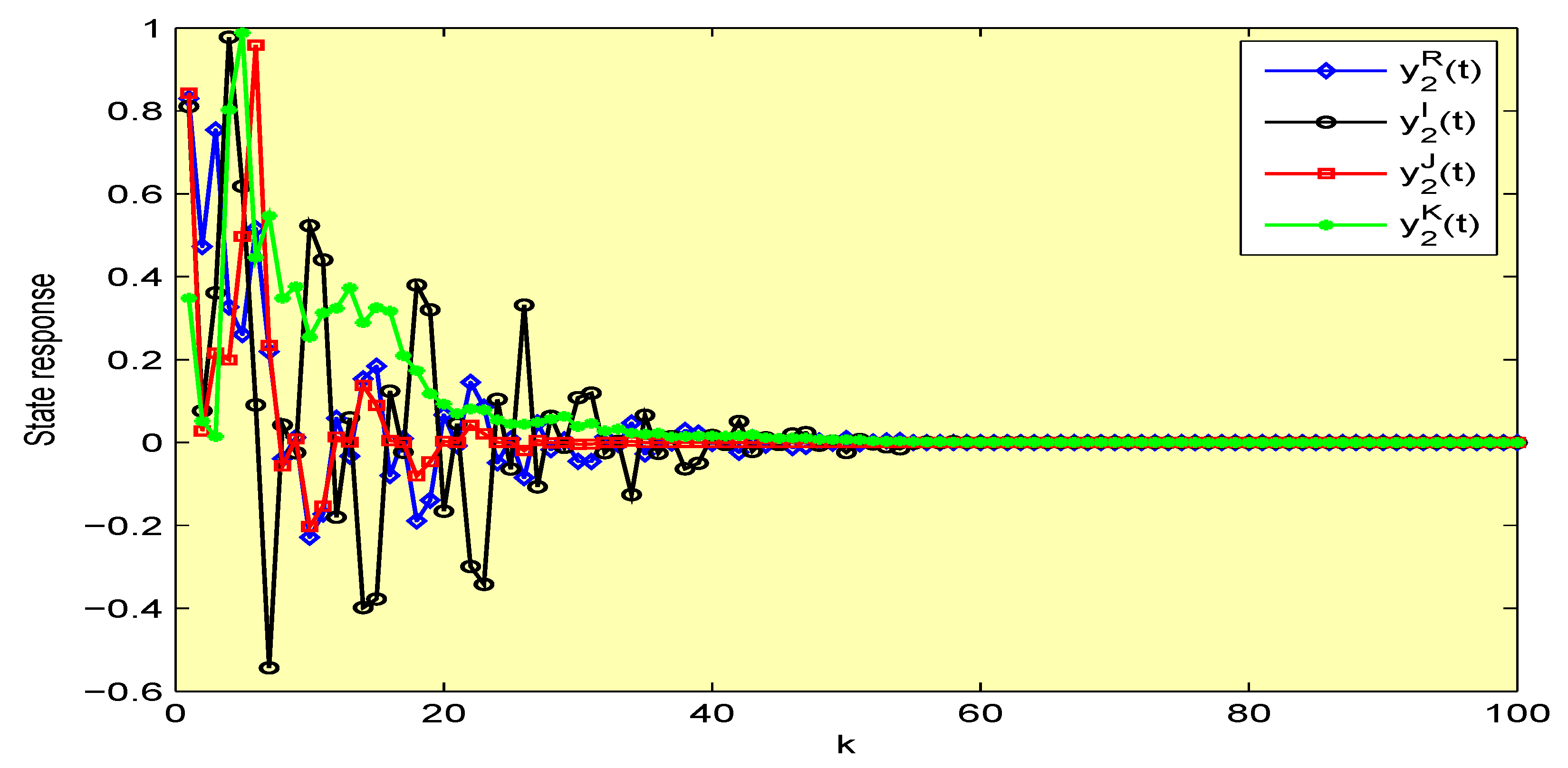
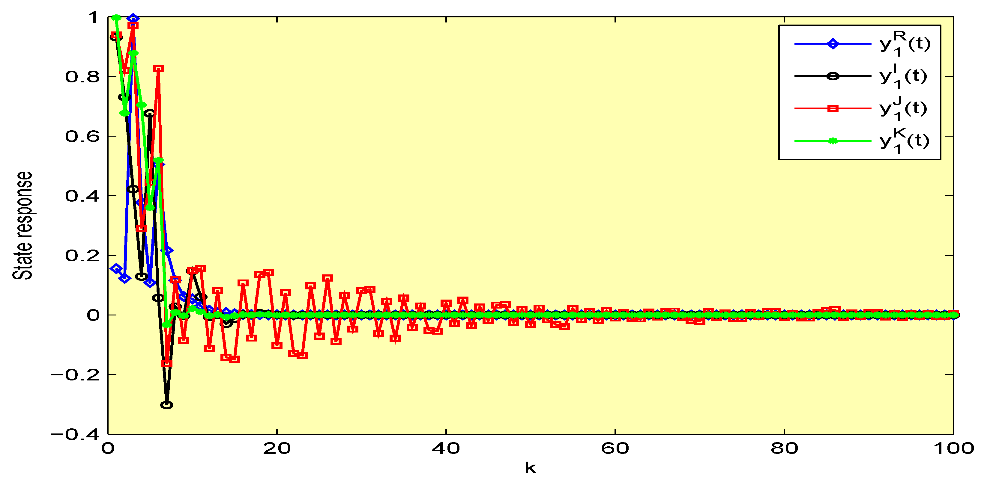
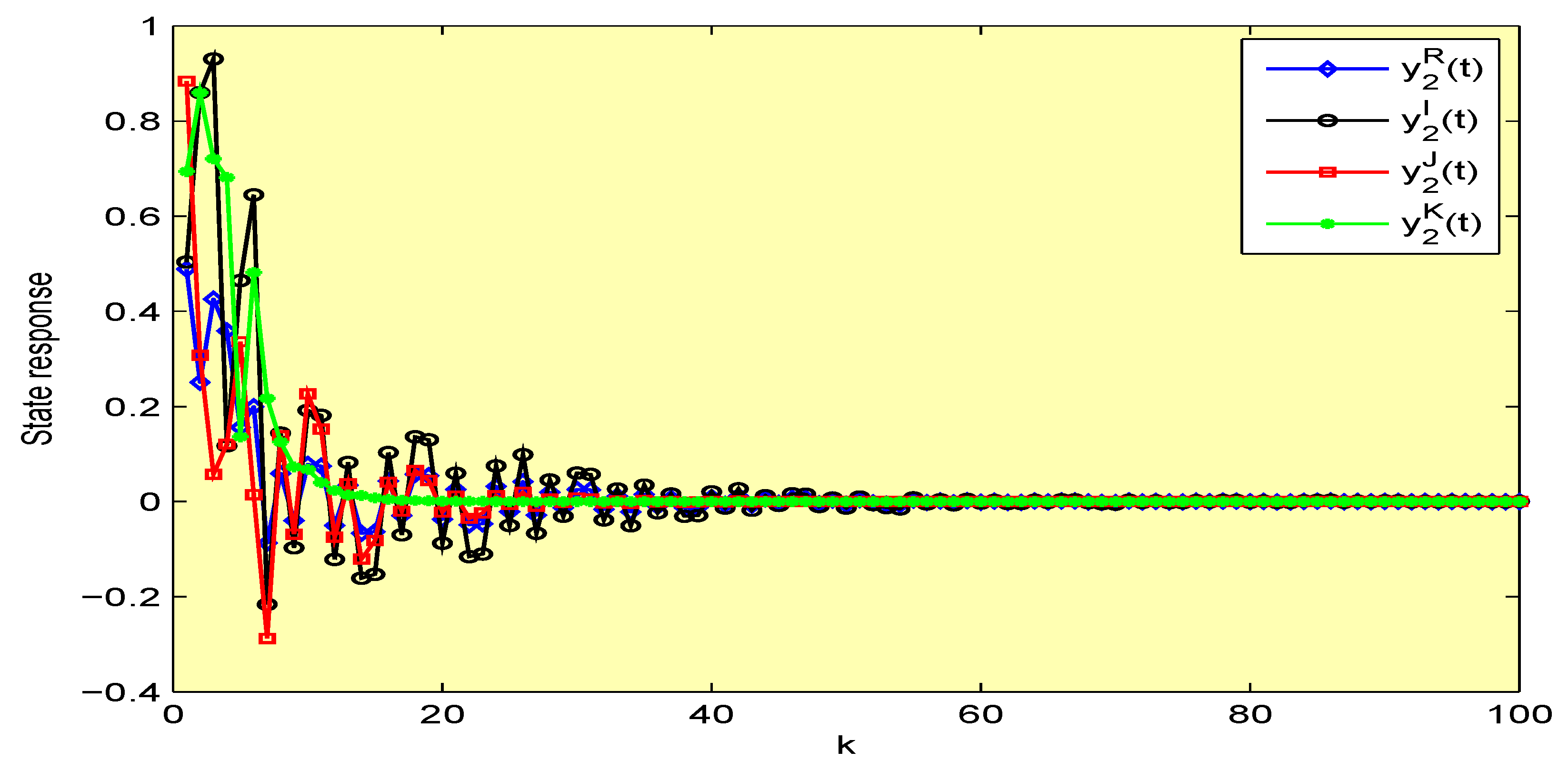
In view of Theorem (1), it is easy to conclude that the NN model in (8) with the above given parameters is mean-square asymptotically stable based on the Lyapunov stability theory. The state trajectories y 1 R ( k ) , y 1 I ( k ) , y 1 J ( k ) , y 1 K ( k ) , y 2 R ( k ) , y 2 I ( k ) , y 2 J ( k ) , y 2 K ( k ) of the NN model in (8) with stochastic disturbances are depicted in Figure 1 and Figure 2, respectively. Figure 3 and Figure 4 show the state trajectories y 1 R ( k ) , y 1 I ( k ) , y 1 J ( k ) , y 1 K ( k ) , y 2 R ( k ) , y 2 I ( k ) , y 2 J ( k ) , y 2 K ( k ) of the NN model in (8) without stochastic disturbances.
Example 2.
The following parameters pertaining to the NN model in (27) are considered:
D = 0.2 0 0 0.2 , A = 0.5 + 0.8 i 0.6 0.4 i 0.7 + 0.5 i 0.3 + 0.2 i .
By separating the activation function into both real and imaginary parts, we obtain A R and A I . The noise intensity functions are considered as σ R ( k , y R ( k ) ) = 0.1 y R ( k ) , σ I ( k , y I ( k ) ) = 0.1 y I ( k ) ; we can verify that A4 is satisfied with ρ 1 = ρ 2 = 0.02 . Take the time-delay ς = 3 , and subject to the following activation functions
f ( y ) = f 1 R ( y 1 R ) + i f 1 I ( y 1 I ) f 2 R ( y 2 R ) + i f 2 I ( y 2 I ) ,
with
f ( y ) = t a n h ( 0.2 y 1 R ) + i t a n h ( 0.2 y 1 I ) t a n h ( 0.2 y 2 R ) + i t a n h ( 0.2 y 2 I ) .
It can verified that A3 is satisfied with ξ 1 R = ξ 1 I = 0.1 , ξ 1 R + = ξ 1 I + = 0.1 , ξ 2 R = ξ 2 I = 0.2 , ξ 2 R + = ξ 2 I + = 0.2 ,
Υ 1 = Γ 1 = 0.01 0 0 0.04 , Υ 2 = Γ 2 = 0 0 0 0 .
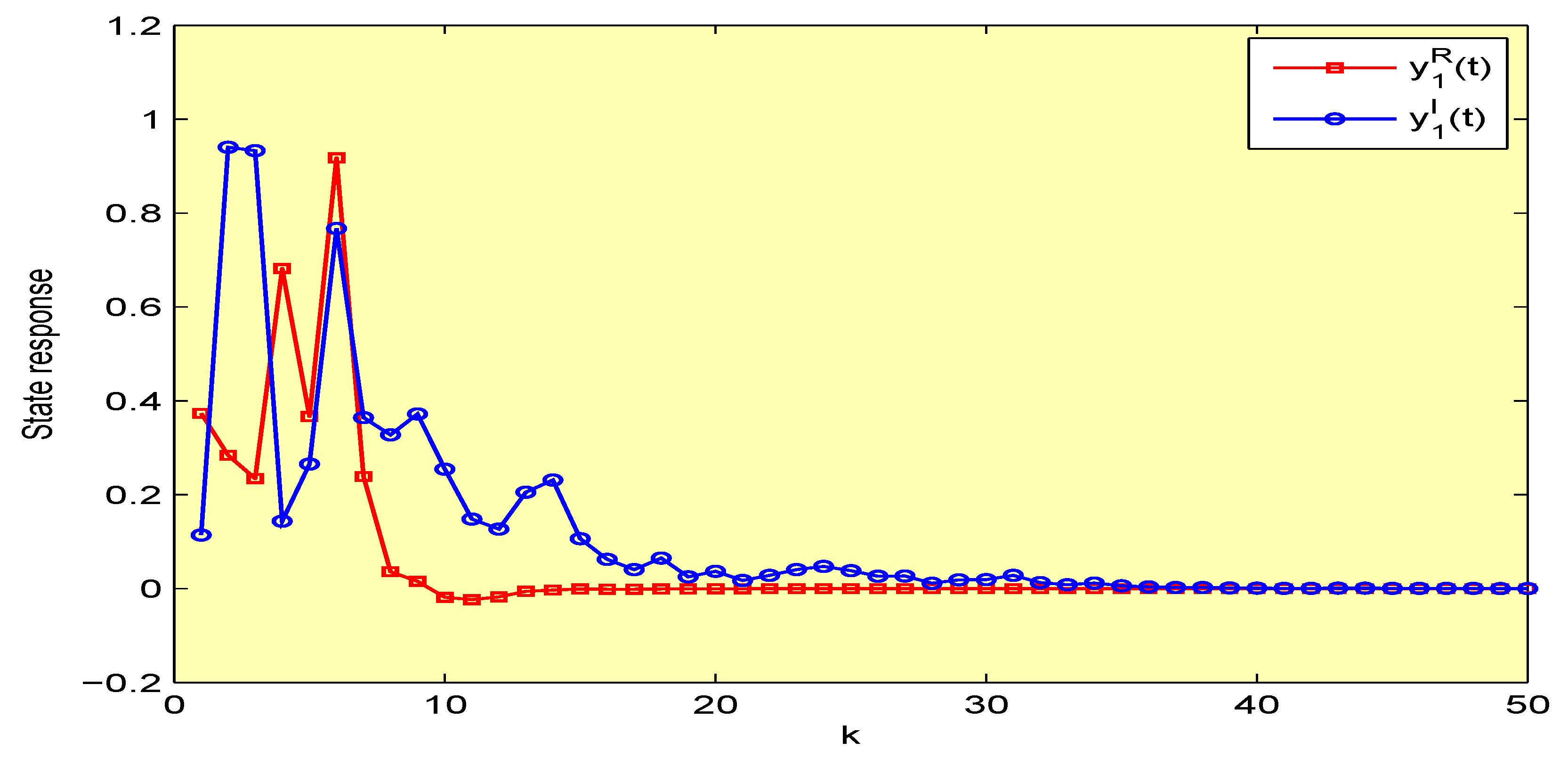
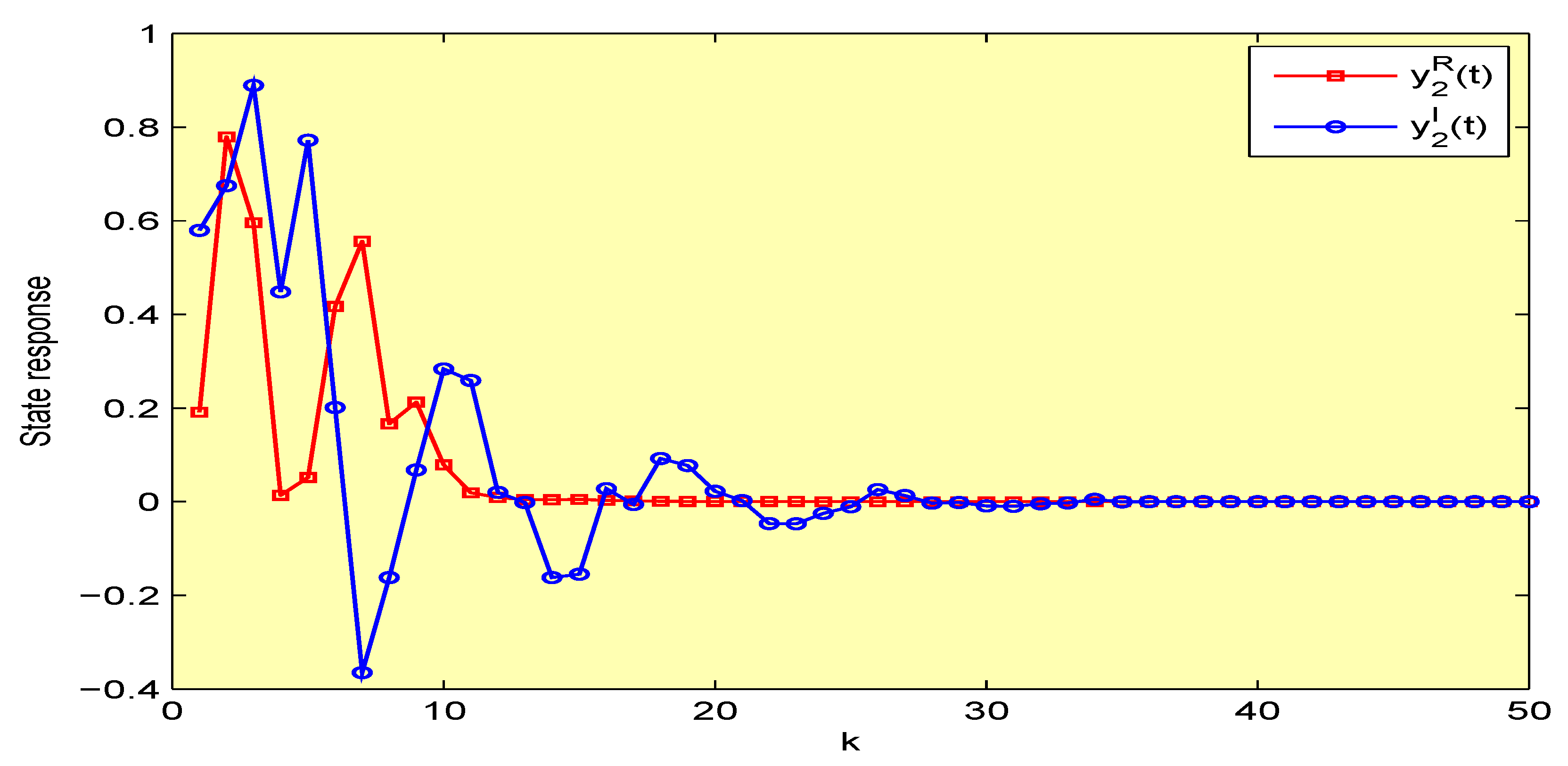
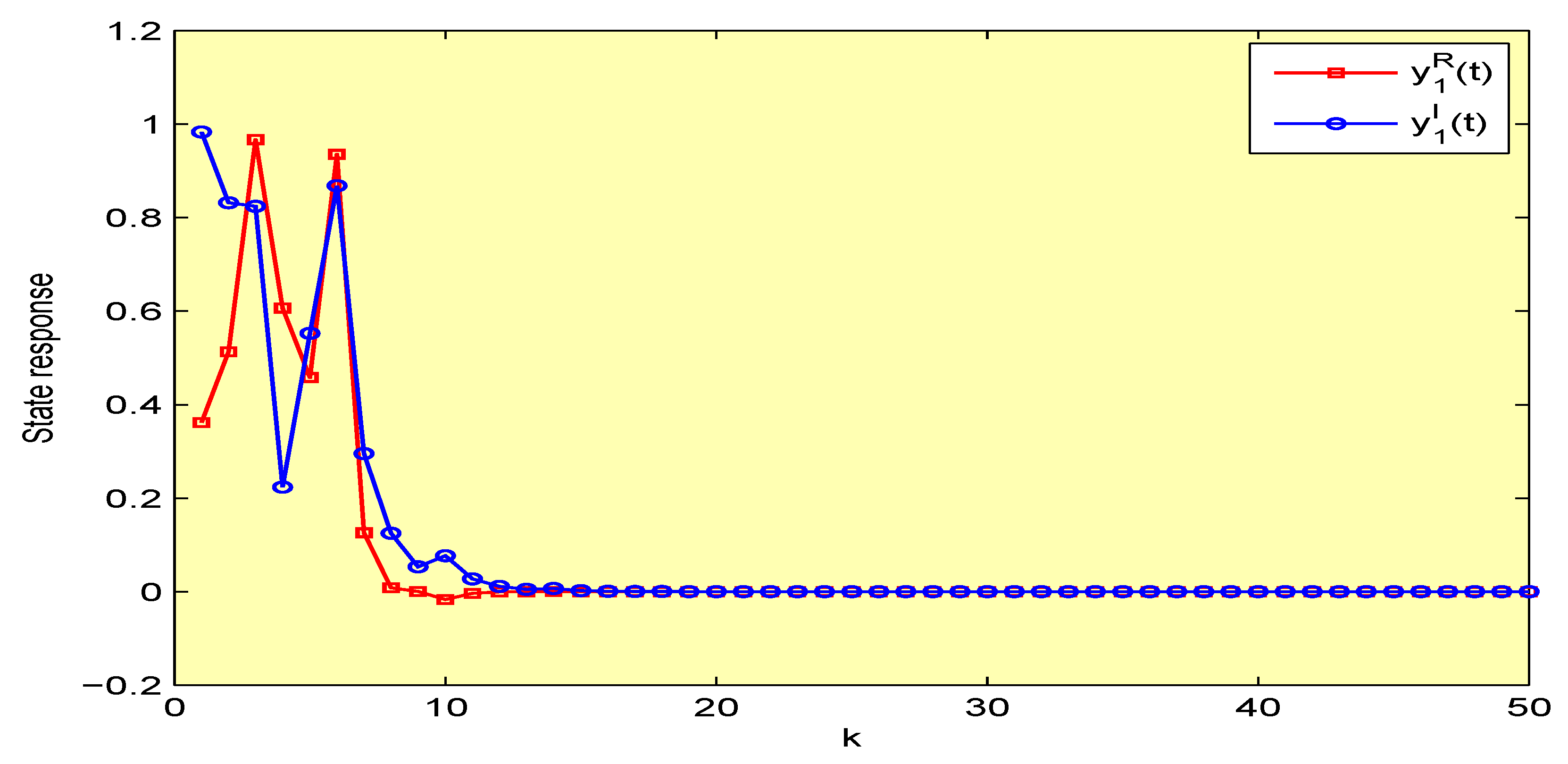
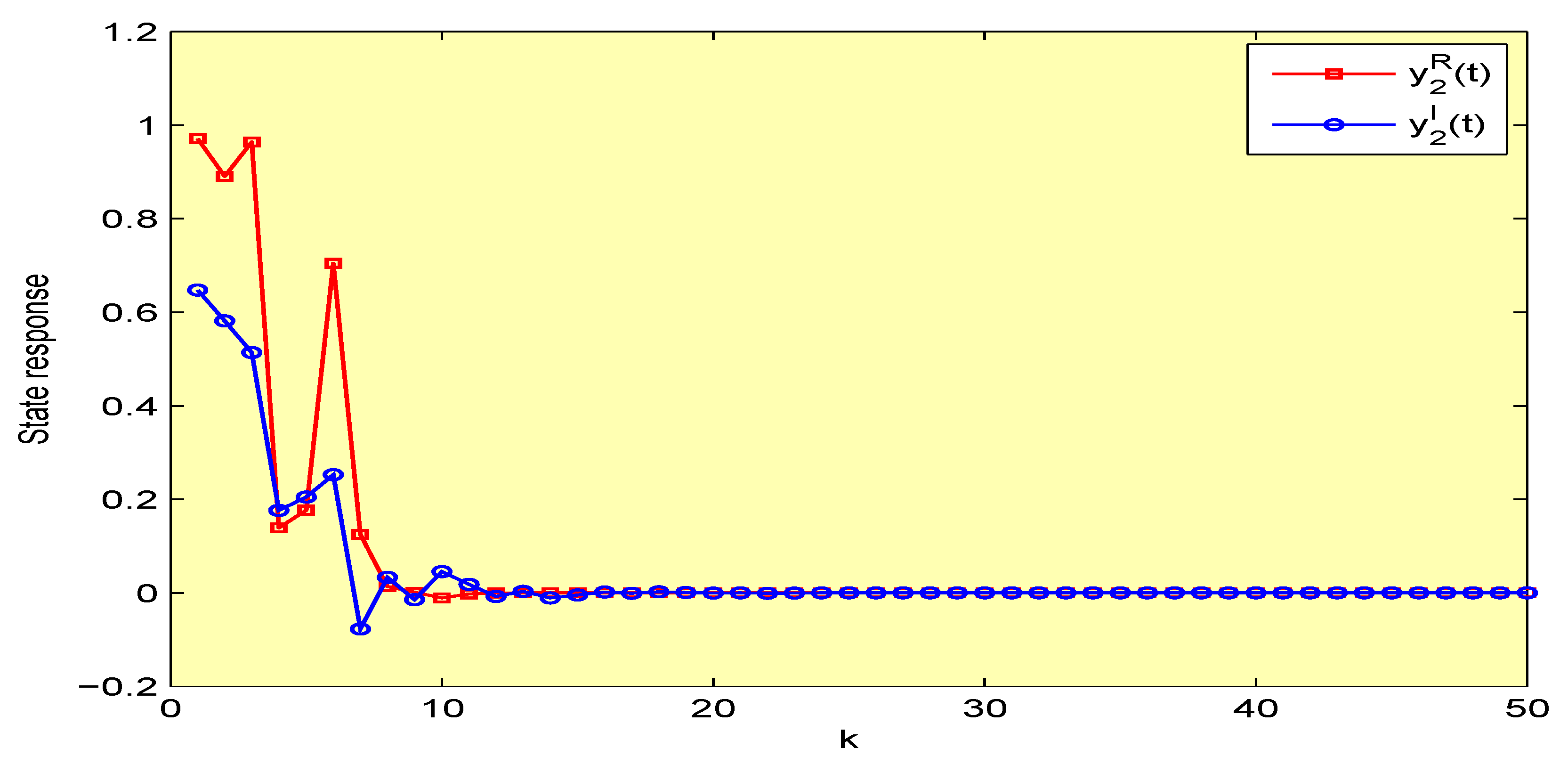
We can find that the conditions (30)–(33) are true by using the LMI control toolbox in MATLAB. According to Corollary (2), we can conclude that the NN model in (27) with the aforementioned parameters is asymptotically stable in the mean square sense based on the Lyapunov stability theory. The state trajectories y 1 R ( k ) , y 1 I ( k ) , y 2 R ( k ) , y 2 I ( k ) of the NN model in (27) with stochastic disturbances are depicted in Figure 5 and Figure 6, respectively. Figure 7 and Figure 8 show the state trajectories y 1 R ( k ) , y 1 I ( k ) , y 2 R ( k ) , y 2 I ( k ) of the NN model in (27) without stochastic disturbances.

5. Conclusions

In this study, we have investigated the mean-square asymptotic stability criteria for the considered DSQVNN models. The designed DSQVNN models encompass discrete-time stochastic CVNN and discrete-time stochastic RVNN as the special cases. By exploiting the real-imaginary separation method, we have derived four equivalent RVNNs from the original QVNN model. By formulating appropriate Lyapunov functional candidates with more system information, and by employing stochastic concepts, we have established the LMI-based new sufficient conditions for the mean-square asymptotic stability of the DSQVNN models. It is worth noting that previously known results can be treated as special cases in our results. The effectiveness of our investigation has been demonstrated through numerical examples.
For future work, a variety of stochastic QVNN models will be examined. Specifically, the BAM (bidirectional associative memory)-type and Cohen–Grossberg-type of QVNN model under the discrete-time case will be investigated in our next study.

Author Contributions

Conceptualization, G.R., R.S. (Ramalingam Sriraman), and P.C.; formal analysis, G.R. and R.S. (Ramalingam Sriraman); funding acquisition, P.C.; investigation, G.R.; methodology, G.R. and R.S. (Ramalingam Sriraman); resources, G.R.; software, P.C., R.S. (Ramalingam Sriraman), and R.S. (Rajendran Samidurai); supervision, C.P.L.; validation, G.R. and R.S. (Ramalingam Sriraman); writing—original draft, G.R.; writing—review and editing, G.R. All authors have read and agreed to the published version of the manuscript.

Funding

This research is made possible through financial support from Chiang Mai University.

Acknowledgments

The authors are grateful to Chiang Mai University for supporting this research.

Conflicts of Interest

The authors declare no conflicts of interest.

Appendix A

Proof of Theorem
(1). Given the NN model in (11), the following Lyapunov functional candidate is considered
V ( k ) = = 1 3 V R ( k ) + V I ( k ) + V J ( k ) + V K ( k ) ,
where
V 1 R ( k ) = ( y R ( k ) ) T P 1 y R ( k ) , V 1 I ( k ) = ( y I ( k ) ) T P 2 y I ( k ) , V 1 J ( k ) = ( y J ( k ) ) T P 3 y J ( k ) , V 1 K ( k ) = ( y K ( k ) ) T P 4 y K ( k ) , V 2 R ( k ) = u = k ς k 1 ( y R ( u ) ) T Q 1 y R ( u ) , V 2 I ( k ) = u = k ς k 1 ( y I ( u ) ) T Q 2 y I ( u ) , V 2 J ( k ) = u = k ς k 1 ( y J ( u ) ) T Q 3 y J ( u ) , V 2 K ( k ) = u = k ς k 1 ( y K ( u ) ) T Q 4 y K ( u ) , V 3 R ( k ) = ς u = ς 1 v = k + u k 1 ( y R ( v ) ) T R 1 y R ( v ) , V 3 I ( k ) = ς u = ς 1 v = k + u k 1 ( y I ( v ) ) T R 2 y I ( v ) , V 3 J ( k ) = ς u = ς 1 v = k + u k 1 ( y J ( v ) ) T R 3 y J ( v ) , V 3 K ( k ) = ς u = ς 1 v = k + u k 1 ( y K ( v ) ) T R 4 y K ( v ) .
The following expression can be obtained when we compute the difference of V ( k ) with respect to the the NN model in (11), and take the mathematical expectation:
E { V ( k ) } = = 1 3 E { V R ( k ) } + E { V I ( k ) } + E { V J ( k ) } + E { V K ( k ) } ,
where
E { V 1 R ( k ) } = E { V 1 R ( k + 1 ) V 1 R ( k ) } = E { [ D y R ( k ) + A R f R ( y R ( k ς ) ) A I f I ( y I ( k ς ) ) A J f J ( y J ( k ς ) ) A K f K ( y K ( k ς ) ) ] T P 1 [ D y R ( k ) + A R f R ( y R ( k ς ) ) A I f I ( y I ( k ς ) ) A J f J ( y J ( k ς ) ) A K f K ( y K ( k ς ) ) ] + ( σ R ( k , y R ( k ) ) ) T P 1 σ R ( k , y R ( k ) ) ( y R ( k ) ) T P 1 y R ( k ) } = E { ( y R ( k ) ) T ( D T P 1 D ) y R ( k ) + 2 ( y R ( k ) ) T ( D T P 1 A R ) f R ( y R ( k ς ) ) 2 ( y R ( k ) ) T ( D T P 1 A I ) f I ( y I ( k ς ) ) 2 ( y R ( k ) ) T ( D T P 1 A J ) f J ( y J ( k ς ) ) 2 ( y R ( k ) ) T ( D T P 1 A K ) f K ( y K ( k ς ) ) + ( f R ( y R ( k ς ) ) ) T ( ( A R ) T P 1 A R ) × f R ( y R ( k ς ) ) 2 ( f R ( y R ( k ς ) ) ) T ( ( A R ) T P 1 A I ) f I ( y I ( k ς ) ) 2 ( f R ( y R ( k ς ) ) ) T ( ( A R ) T P 1 A J ) f J ( y J ( k ς ) ) 2 ( f R ( y R ( k ς ) ) ) T × ( ( A R ) T P 1 A K ) f K ( y K ( k ς ) ) + ( f I ( y I ( k ς ) ) ) T ( ( A I ) T P 1 A I ) f I ( y I ( k ς ) ) + 2 ( f I ( y I ( k ς ) ) ) T ( ( A I ) T P 1 A J ) f J ( y J ( k ς ) ) + 2 ( f I ( y I ( k ς ) ) ) T ( ( A I ) T P 1 A K ) × f K ( y K ( k ς ) ) + ( f J ( y J ( k ς ) ) ) T ( ( A J ) T P 1 A J ) f J ( y J ( k ς ) ) + 2 ( f J ( y J ( k ς ) ) ) T × ( ( A J ) T P 1 A K ) f K ( y K ( k ς ) ) + ( f K ( y K ( k ς ) ) ) T ( ( A K ) T P 1 A K ) f K ( y K ( k ς ) ) + ( σ R ( k , y R ( k ) ) T P 1 σ R ( k ) ) ( y R ( k ) ) T ( P 1 ) y R ( k ) } ,
E { V 1 I ( k ) } = E { V 1 I ( k + 1 ) V 1 I ( k ) } = E { [ D y I ( k ) + A R f I ( y I ( k ς ) ) + A I f R ( y R ( k ς ) ) + A I f K ( y K ( k ς ) ) A K f J ( y J ( k ς ) ) ] T P 2 [ D y I ( k ) + A R f I ( y I ( k ς ) ) + A I f R ( y R ( k ς ) ) + A J f K ( y K ( k ς ) ) A K f J ( y J ( k ς ) ) ] + ( σ I ( k , y I ( k ) ) ) T P 2 σ I ( k , y I ( k ) ) ( y I ( k ) T P 2 y I ( k ) } = E { ( y I ( k ) ) T ( D T P 2 D ) y I ( k ) + 2 ( y I ( k ) ) T ( D T P 2 A R ) f I ( y I ( k ς ) ) + 2 ( y I ( k ) ) T ( D T P 2 A I ) f R ( y R ( k ς ) ) + 2 ( y I ( k ) ) T ( D T P 2 A J ) f K ( y K ( K ς ) ) 2 ( y I ( k ) ) T ( D T P 2 A K ) f J ( y J ( k ς ) ) + ( f I ( y I ( k ς ) ) ) T ( ( A R ) T P 2 A R ) × f I ( y I ( k ς ) ) + 2 ( f I ( y I ( k ς ) ) ) T ( ( A R ) T P 2 A I ) f R ( y R ( k ς ) ) + 2 ( f I ( y I ( k ς ) ) ) T ( ( A R ) T P 2 A J ) f K ( y K ( k ς ) ) 2 f I ( y I ( k ς ) ) ) T × ( ( A R ) T P 2 A K ) f J ( y J ( k ς ) ) + ( f R ( y R ( k ς ) ) ) T ( ( A I ) T P 2 A I ) f R ( y R ( k ς ) ) + 2 ( f R ( y R ( k ς ) ) ) T ( ( A I ) T P 2 A J ) f K ( y K ( k ς ) ) 2 ( f R ( y R ( k ς ) ) ) T × ( ( A I ) T P 2 A K ) f I ( y I ( k ς ) ) + ( f K ( y K ( k ς ) ) ) T ( ( A J ) T P 2 A J ) f K ( y K ( k ς ) ) 2 ( f K ( y K ( k ς ) ) ) T ( ( A J ) T P 2 A K ) f J ( y J ( k ς ) ) + ( f J ( y J ( k ς ) ) ) T × ( ( A K ) T P 2 A K ) f J ( y J ( k ς ) ) + ( σ I ( k , y I ( k ) ) ) T P 2 σ I ( k , y I ( k ) ) ( y I ( k ) ) T ( P 2 ) y I ( k ) } ,
E { V 1 J ( k ) } = E { V 1 J ( k + 1 ) V 1 J ( k ) } = E { [ D y J ( k ) + A R f J ( y J ( k ς ) ) + A J f R ( y R ( k ς ) ) + A K f I ( y I ( k ς ) ) A I f K ( y K ( k ς ) ) ] T P 3 [ D y J ( k ) + A R f J ( y J ( k ς ) ) + A J f R ( y R ( k ς ) ) + A K f I ( y I ( k ς ) ) A I f K ( y K ( k ς ) ) ] + ( σ J ( k , y J ( k ) ) ) T P 3 σ J ( k , y J ( k ) ) ( y J ( k ) T P 3 y J ( k ) } = E { ( y J ( k ) ) T ( D T P 3 D ) y J ( k ) + 2 ( y J ( k ) ) T ( D T P 3 A R ) f J ( y J ( k ς ) ) + 2 ( y J ( k ) ) T ( D T P 3 A J ) f R ( y R ( k ς ) ) + 2 ( y J ( k ) ) T ( D T P 3 A K ) f I ( y I ( k ς ) ) 2 ( y J ( k ) ) T ( D T P 3 A I ) f K ( y K ( k ς ) ) + ( f J ( y J ( k ς ) ) ) T ( ( A R ) T P 3 A R ) × f J ( y J ( k ς ) ) + 2 ( f J ( y J ( k ς ) ) ) T ( ( A R ) T P 3 A J ) f R ( y R ( k ς ) ) + 2 ( f J ( y J ( k ς ) ) ) T × ( ( A R ) T P 3 A K ) f I ( y I ( k ς ) ) 2 ( f J ( y J ( k ς ) ) ) T ( ( A R ) T P 3 A I ) f K ( y K ( k ς ) ) + ( f R ( y R ( k ς ) ) ) T ( ( A J ) T P 3 A J ) f R ( y R ( k ς ) ) + 2 ( f R ( y R ( k ς ) ) ) T ( ( A J ) T P 3 A K ) × f I ( y I ( k ς ) ) 2 ( f R ( y R ( k ς ) ) ) T ( ( A J ) T P 3 A I ) f K ( y K ( k ς ) ) + ( f I ( y I ( k ς ) ) ) T × ( ( A K ) T P 3 A K ) f I ( y I ( k ς ) ) 2 ( f I ( y I ( k ς ) ) ) T ( ( A K ) T P 3 A I ) f K ( y K ( k ς ) ) + ( f K ( y K ( k ς ) ) ) T ( ( A I ) T P 3 A I ) f K ( y K ( k ς ) ) + ( σ J ( k , y J ( k ) ) ) T P 3 σ J ( k , y J ( k ) ) ( y J ( k ) ) T ( P 3 ) y J ( k ) } ,
E { V 1 K ( k ) } = E { V 1 K ( k + 1 ) V 1 K ( k ) } = E { [ D y K ( k ) + A R f K ( y K ( k ς ) ) + A K f R ( y R ( k ς ) ) + A I f J ( y J ( k ς ) ) A J f I ( y I ( k ς ) ) ] T P 4 [ D y K ( k ) + A R f K ( y K ( k ς ) ) + A K f R ( y R ( k ς ) ) + A I f J ( y J ( k ς ) ) A J f I ( y I ( k ς ) ) ] + ( σ K ( k , y K ( k ) ) ) T P 4 σ K ( k , y K ( k ) ) ( y K ( k ) ) T P 4 y K ( k ) } = E { ( y K ( k ) ) T ( D T P 4 D ) y K ( k ) + 2 ( y K ( k ) ) T ( D T P 4 A R ) f K ( y K ( k ς ) ) + 2 ( y K ( k ) ) T ( D T P 4 A K ) f R ( y R ( k ς ) ) + 2 ( y K ( k ) ) T ( D T P 4 A I ) f J ( y J ( k ς ) ) 2 ( y K ( k ) ) T ( D T P 4 A J ) f I ( y I ( k ς ) ) + ( f K ( y K ( k ς ) ) ) T ( ( A R ) T P 4 A R ) × f K ( y K ( k ς ) ) + 2 ( f K ( y K ( k ς ) ) ) T ( ( A R ) T P 4 A K ) f R ( y R ( k ς ) ) + 2 ( f K ( y K ( k ς ) ) ) T ( ( A R ) T P 4 A I ) f J ( y J ( k ς ) ) 2 ( f K ( y K ( k ς ) ) ) T × ( ( A R ) T P 4 A J ) f I ( y I ( k ς ) ) + ( f R ( y R ( k ς ) ) ) T ( ( A K ) T P 4 A K ) f R ( y R ( k ς ) ) + 2 ( f R ( y R ( k ς ) ) ) T ( ( A K ) T P 4 A I ) f J ( y J ( k ς ) ) 2 ( f R ( y R ( k ς ) ) ) T ( ( A K ) T P 4 A J ) × f I ( y I ( k ς ) ) + ( f J ( y J ( k ς ) ) ) T ( ( A I ) T P 4 A I ) f J ( y J ( k ς ) ) 2 ( f J ( y J ( k ς ) ) ) T × ( ( A I ) T P 4 A J ) f I ( y I ( k ς ) ) + ( f I ( y I ( k ς ) ) ) T ( ( A J ) T P 4 A J ) f I ( y I ( k ς ) ) + ( σ K ( k , y K ( k ) ) T P 4 σ K ( k , y K ( k ) ) ( y K ( k ) ) T ( P ) y R ( k ) } ,
Similarly, the following can be obtained:
E { V 2 R ( k ) } = E { V 2 R ( k + 1 ) V 2 R ( k ) } = ( y R ( k ) ) T Q 1 y R ( k ) ( y R ( k ς ) ) T Q 1 y R ( k ς ) ,
E { V 2 I ( k ) } = E { V 2 I ( k + 1 ) V 2 I ( k ) } = ( y I ( k ) ) T Q 2 y I ( k ) ( y I ( k ς ) ) T Q 2 y I ( k ς ) ,
E { V 2 J ( k ) } = E { V 2 J ( k + 1 ) V 2 J ( k ) } = ( y J ( k ) ) T Q 3 y J ( k ) ( y J ( k ς ) ) T Q 3 y J ( k ς ) ,
E { V 2 K ( k ) } = E { V 2 K ( k + 1 ) V 2 K ( k ) } = ( y R ( k ) ) T Q 4 y R ( k ) ( y R ( k ς ) ) T Q 4 y R ( k ς ) ,
E { V 3 R ( k ) } = E { V 3 R ( k + 1 ) V 3 R ( k ) } = E ς u = ς 1 v = k + u + 1 k ( y R ( v ) ) T R 1 y R ( v ) ς u = ς 1 v = k + u k 1 ( y R ( v ) ) T R 1 y R ( v ) = ς 2 ( y R ( k ) ) T R 1 y R ( k ) ς u = k ς k 1 ( y R ( u ) ) T R 1 y R ( u ) ,
E { V 3 I ( k ) } = E { V 3 I ( k + 1 ) V 3 I ( k ) } = E ς u = ς 1 v = k + u + 1 k ( y I ( v ) ) T R 2 y I ( v ) ς u = ς 1 v = k + u k 1 ( y I ( v ) ) T R 2 y I ( v ) = ς 2 ( y I ( k ) ) T R 2 y I ( k ) ς u = k ς k 1 ( y I ( u ) ) T R 2 y I ( u ) ,
E { V 3 J ( k ) } = E { V 3 J ( k + 1 ) V 3 J ( k ) } = E ς u = ς 1 v = k + u + 1 k ( y J ( v ) ) T R 3 y J ( v ) ς u = ς 1 v = k + u k 1 ( y J ( v ) ) T R 3 y J ( v ) = ς 2 ( y J ( k ) ) T R 3 y J ( k ) ς u = k ς k 1 ( y J ( u ) ) T R 3 y J ( u ) ,
E { V 3 K ( k ) } = E { V 3 K ( k + 1 ) V 3 K ( k ) } = E ς u = ς 1 v = k + u + 1 k ( y K ( v ) ) T R 4 y K ( v ) ς u = ς 1 v = k + u k 1 ( y K ( v ) ) T R 4 y K ( v ) = ς 2 ( y K ( k ) ) T R 4 y K ( k ) ς u = k ς k 1 ( y K ( u ) ) T R 4 y K ( u ) ,
By using Lemma (1), we have
ς u = k ς k 1 ( y K ( u ) ) T R 1 y K ( u ) u = k ς k 1 ( y K ( u ) ) T R 1 u = k ς k 1 y K ( u ) ,
ς u = k ς k 1 ( y K ( u ) ) T R 2 y K ( u ) u = k ς k 1 ( y K ( u ) ) T R 2 u = k ς k 1 y K ( u ) ,
ς u = k ς k 1 ( y K ( u ) ) T R 3 y K ( u ) u = k ς k 1 ( y K ( u ) ) T R 3 u = k ς k 1 y K ( u ) ,
ς u = k ς k 1 ( y K ( u ) ) T R 4 y K ( u ) u = k ς k 1 ( y K ( u ) ) T R 4 u = k ς k 1 y K ( u ) .
From A2 and conditions (13)–(16), we have
( σ R ( k , y R ( k ) ) ) T P 1 σ R ( k , y R ( k ) ) λ 1 m a x ( P 1 ) ( σ R ( k , y R ( k ) ) ) T σ R ( k , y R ( k ) ) λ 1 ρ 1 ( y R ( k ) ) T y R ( k ) ,
( σ I ( k , y I ( k ) ) ) T P 3 σ I ( k , y I ( k ) ) λ 2 m a x ( P 2 ) ( σ I ( k , y I ( k ) ) ) T σ I ( k , y I ( k ) ) λ 2 ρ 2 ( y I ( k ) ) T y I ( k ) ,
( σ J ( k , y J ( k ) ) ) T P 3 σ J ( k , y J ( k ) ) λ 3 m a x ( P 3 ) ( σ J ( k , y J ( k ) ) ) T σ J ( k , y J ( k ) ) λ 3 ρ 3 ( y J ( k ) ) T y J ( k ) ,
( σ K ( k , y K ( k ) ) ) T P 4 σ K ( k , y K ( k ) ) λ 4 m a x ( P 4 ) ( σ K ( k , y K ( k ) ) ) T σ K ( k , y K ( k ) ) λ 4 ρ 4 ( y K ( k ) ) T y K ( k ) .
From A1, we have
( f q R ( y q R ( k ) ) ξ q R + y q R ( k ) ) ( f q R ( y q R ( k ) ) ξ q R y q R ( k ) ) 0 , ( f q I ( y q I ( k ) ) ξ q I + y q I ( k ) ) ( f q I ( y q I ( k ) ) ξ q I y q I ( k ) ) 0 , ( f q J ( y q J ( k ) ) ξ q J + y q J ( k ) ) ( f q J ( y q J ( k ) ) ξ q J y q J ( k ) ) 0 , ( f q K ( y q K ( k ) ) ξ q K + y q K ( k ) ) ( f q K ( y q K ( k ) ) ξ q K y q K ( k ) ) 0 , q = 1 , , m ,
which is equivalent to
y R ( k ς ) f R ( y R ( k ς ) ) T ξ q R + ξ q R e q e q T ξ q R + + ξ q R 2 e q e q T ξ q R + + ξ q R 2 e q e q T e q e q T y R ( k ς ) f R ( y R ( k ς ) ) 0 ,
y I ( k ς ) f I ( y I ( k ς ) ) T ξ q I + ξ q I e q e q T ξ q I + + ξ q I 2 e q e q T ξ q I + + ξ q I 2 e q e q T e q e q T y I ( k ς ) f I ( y I ( k ς ) ) 0 ,
y J ( k ς ) f J ( y J ( k ς ) ) T ξ q J + ξ q J e q e q T ξ q J + + ξ q J 2 e q e q T ξ q J + + ξ q J 2 e q e q T e q e q T y J ( k ς ) f J ( y J ( k ς ) ) 0 ,
y K ( k ς ) f K ( y K ( k ς ) ) T ξ q K + ξ q K e q e q T ξ q K + + ξ q K 2 e q e q T ξ q K + + ξ q K 2 e q e q T e q e q T y K ( k ς ) f K ( y K ( k ς ) ) 0 ,
for all q = 1 , , m , while the unit column vector having one element on its q-th row and zeros elsewhere is denoted by e q .
Subject to the existence of L 1 = d i a g { l 1 R , , l m R } , we can conclude from (A23) that
q = 1 n l q R y R ( k ς ) f R ( y R ( k ς ) ) T ξ q R + ξ q R e q e q T ξ q R + + ξ q R 2 e q e q T ξ q R + + ξ q R 2 e q e q T e q e q T y R ( k ς ) f R ( y R ( k ς ) ) 0 ,
that is
y R ( k ς ) f R ( y R ( k ς ) ) T Υ 1 L 1 Υ 2 R L 1 Υ 2 L 1 L 1 y R ( k ς ) f R ( y R ( k ς ) ) 0 ,
In a similar way to (A24)–(A26) for which there exist L 2 = d i a g { l 1 I , , l m I } , L 3 = d i a g { l 1 J , , l m J } , L 4 = d i a g { l 1 K , , l m K } , we have
y I ( k ς ) f I ( y I ( k ς ) ) T Γ 1 L 2 Γ 2 L 2 Γ 2 L 2 L 2 y I ( k ς ) f I ( y I ( k ς ) ) 0 ,
y J ( k ς ) f J ( y J ( k ς ) ) T Λ 1 L 3 Λ 2 L 3 Λ 2 L 3 L 3 y J ( k ς ) f J ( y J ( k ς ) ) 0 ,
y K ( k ς ) f K ( y K ( k ς ) ) T Π 1 L 4 Π 2 L 4 Π 2 L 4 L 4 y K ( k ς ) f K ( y K ( k ς ) ) 0 ,
where Υ 1 = d i a g ξ 1 R + ξ 1 R , , ξ m R + ξ m R , Υ 2 = d i a g ξ 1 R + + ξ 1 R 2 , , ξ m R + + ξ m R 2 ,
  • Γ 1 = d i a g ξ 1 I + ξ 1 I , , ξ m I + ξ m I , Γ 2 = d i a g ξ 1 I + + ξ 1 I 2 , , ξ m + + ξ m I 2 ,
  • Λ 1 = d i a g ξ 1 J + ξ 1 J , , ξ m J + ξ m J , Λ 2 = d i a g ξ 1 J + + ξ 1 J 2 , , ξ m J + + ξ m J 2 ,
  • Π 1 = d i a g ξ 1 K + ξ 1 K , , ξ m K + ξ m K , Π 2 = d i a g ξ 1 K + + ξ 1 K 2 , , ξ m K + + ξ m K 2
By simple computation, it follows from (A3)–(A31) that
E { V ( k ) } ζ 1 T ( k ) Θ 1 ζ 1 ( k ) + ζ 2 T ( k ) Θ 2 ζ 2 ( k ) + ζ 3 T ( k ) Θ 3 ζ 3 ( k ) + ζ 4 T ( k ) Θ 4 ζ 4 ( k ) < 0 ,
where
ζ 1 ( k ) = [ ( y R ( k ) ) T , ( y R ( k ς ) ) T , ( f R ( y R ( k ς ) ) ) T , ( f I ( y I ( k ς ) ) ) T , ( f J ( y J ( k ς ) ) ) T , ( f K ( y K ( k ς ) ) ) T , u = k ς k 1 ( y R ( u ) ) T ] T , ζ 2 ( k ) = [ ( y I ( k ) ) T , ( y I ( k ς ) ) T , ( f R ( y R ( k ς ) ) ) T , ( f I ( y I ( k ς ) ) ) T , ( f J ( y J ( k ς ) ) ) T , ( f K ( y K ( k ς ) ) ) T , u = k ς k 1 ( y I ( u ) ) T ] T , ζ 3 ( k ) = [ ( y J ( k ) ) T , ( y J ( k ς ) ) T , ( f R ( y R ( k ς ) ) ) T , ( f I ( y I ( k ς ) ) ) T , ( f J ( y J ( k ς ) ) ) T , ( f K ( y K ( k ς ) ) ) T , u = k ς k 1 ( y J ( u ) ) T ] T , ζ 4 ( k ) = [ ( y K ( k ) ) T , ( y K ( k ς ) ) T , ( f R ( y R ( k ς ) ) ) T , ( f I ( y I ( k ς ) ) ) T , ( f J ( y J ( k ς ) ) ) T , ( f K ( y K ( k ς ) ) ) T , u = k ς k 1 ( y K ( u ) ) T ] T ,
and Θ 1 , Θ 2 , Θ 3 , and Θ 4 are defined in Theorem (1).
Consider the right-hand side of the inequalities (13)–(21), we have Θ 1 < 0 , Θ 2 < 0 , Θ 3 < 0 , and Θ 4 < 0 .
Let α = α m a x ( Θ 1 ) < 0 , β = β m a x ( Θ 2 ) < 0 , γ = γ m a x ( Θ 3 ) < 0 , ϵ = ϵ m a x ( Θ 4 ) < 0 . This fact, together with (A32), yields
E { V ( k ) } α E { y R ( k ) 2 } + β E { y I ( k ) 2 } + γ E { y J ( k ) 2 } + ϵ E { y K ( k ) 2 } ,
for all y R ( k ) , y I ( k ) , y J ( k ) , y K ( k ) 0 . Put ϑ = m a x { α , β , γ , ϵ }
E { V ( k ) } ϑ E { y R ( k ) 2 + y I ( k ) 2 + y J ( k ) 2 + y K ( k ) 2 } ,
which is equivalent to
E { V ( k ) } ϑ E { y ( k ) 2 } .
Consider a positive integer of N. We can have the following expression by summing both sides of (A35) from 0 to N with respect to k
E { V ( N ) V ( 0 ) } ϑ k = 0 N E { y ( k ) 2 } ,
This indicates that
k = 0 N E { y ( k ) 2 } ϑ 1 ( E { V ( N ) } E { V ( 0 ) } ) , ϑ 1 E { V ( 0 ) } .
Since the series k = 0 + E { y ( k ) 2 } is concluded to be convergent, we have
lim k E { y ( k ) 2 } = 0 .
According to Definition 2 the NN model in (11) is asymptotically stable in the mean-square sense. □

References

  1. Feng, C.; Plamondon, R. On the stability analysis of delayed neural networks systems. Neural Netw. 2001, 14, 1181–1188. [Google Scholar] [CrossRef]
  2. Kwon, O.M.; Park, J.H. Exponential stability analysis for uncertain neural networks with interval time-varying delays. Appl. Math. Comput. 2009, 212, 530–541. [Google Scholar] [CrossRef]
  3. Cao, J.; Wang, J. Global asymptotic stability of a general class of recurrent neural networks with time-varying delays. IEEE Trans. Circuits Syst. I 2003, 50, 34–44. [Google Scholar]
  4. Gunasekaran, N.; Syed Ali, M.; Pavithra, S. Finite-time L performance state estimation of recurrent neural networks with sampled-data signals. Neural Process. Lett. 2020, 51, 1379–1392. [Google Scholar] [CrossRef]
  5. Syed Ali, M.; Gunasekaran, N.; Esther Rani, M. Robust stability of Hopfield delayed neural networks via an augmented L-K functional. Neurocomputing 2017, 19, 1198–1204. [Google Scholar] [CrossRef]
  6. Mohamad, S. Global exponential stability in continuous-time and discrete-time delayed bidirectional neural networks. Phys. D 2001, 159, 233–251. [Google Scholar] [CrossRef]
  7. Mohamad, S.; Gopalsamy, K. Exponential stability of continuous-time and discrete-time cellular neural networks with delays. Appl. Math. Comput. 2003, 135, 17–38. [Google Scholar] [CrossRef]
  8. Kwon, O.M.; Park, M.J.; Park, J.H.; Lee, S.M.; Cha, E.J. New criteria on delay-dependent stability for discrete-time neural networks with time-varying delays. Neurocomputing 2013, 121, 185–194. [Google Scholar] [CrossRef]
  9. Liang, J.; Cao, J.; Ho, D.W.C. Discrete-time bidirectional associative memory neural networks with variable delays. Phys. Lett. A 2005, 335, 226–234. [Google Scholar] [CrossRef]
  10. Xiong, W.; Cao, J. Global exponential stability of discrete-time Cohen-Grossberg neural networks. Neurocomputing 2005, 64, 433–446. [Google Scholar] [CrossRef]
  11. Song, Q.; Wang, Z. A delay-dependent LMI approach to dynamics analysis of discrete-time recurrent neural networks with time-varying delays. Phys. Lett. A 2007, 368, 134–145. [Google Scholar] [CrossRef] [Green Version]
  12. Liu, Y.; Wang, Z.; Liu, X. Asymptotic stability for neural networks with mixed time-delays: The discrete-time case. Neural Netw. 2009, 22, 67–74. [Google Scholar] [CrossRef] [Green Version]
  13. Wang, Z.; Liu, Y.; Liu, X.; Shi, Y. Robust state estimation for discrete-time stochastic neural networks with probabilistic measurement delays. Neurocomputing 2010, 74, 256–264. [Google Scholar] [CrossRef]
  14. Samidurai, R.; Sriraman, R.; Cao, J.; Tu, Z. Effects of leakage delay on global asymptotic stability of complex-valued neural networks with interval time-varying delays via new complex-valued Jensen’s inequality. Int. J. Adapt. Control Signal Process. 2018, 32, 1294–1312. [Google Scholar] [CrossRef]
  15. Zhang, Z.; Liu, X.; Zhou, D.; Lin, C.; Chen, J.; Wang, H. Finite-time stabilizability and instabilizability for complex-valued memristive neural networks with time delays. IEEE Trans. Syst. Man Cybern. Syst. 2018, 48, 2371–2382. [Google Scholar] [CrossRef]
  16. Samidurai, R.; Sriraman, R.; Zhu, S. Leakage delay-dependent stability analysis for complex-valued neural networks with discrete and distributed time-varying delays. Neurocomputing 2019, 338, 262–273. [Google Scholar] [CrossRef]
  17. Tu, Z.; Cao, J.; Alsaedi, A.; Alsaadi, F.E.; Hayat, T. Global Lagrange stability of complex-valued neural networks of neutral type with time-varying delays. Complexity 2016, 21, 438–450. [Google Scholar] [CrossRef]
  18. Gunasekaran, N.; Zhai, G. Sampled-data state-estimation of delayed complex-valued neural networks. Int. J. Syst. Sci. 2020, 51, 303–312. [Google Scholar] [CrossRef]
  19. Gunasekaran, N.; Zhai, G. Stability analysis for uncertain switched delayed complex-valued neural networks. Neurocomputing 2019, 367, 198–206. [Google Scholar] [CrossRef]
  20. Zhang, H.; Wang, X.Y.; Lin, X.H.; Liu, C.X. Stability and synchronization for discrete-time complex-valued neural networks with time-varying delays. PLoS ONE 2014, 9, e93838. [Google Scholar] [CrossRef]
  21. Duan, C.; Song, Q. Boundedness and stability for discrete-time delayed neural network with complex-valued linear threshold neurons. Discrete Dyn. Nat. Soc. 2010, 2010, 368379. [Google Scholar] [CrossRef]
  22. Hu, J.; Wang, J. Global exponential periodicity and stability of discrete-time complex-valued recurrent neural networks with time-delays. Neural Netw. 2015, 66, 119–130. [Google Scholar] [CrossRef]
  23. Chen, X.; Song, Q.; Zhao, Z.; Liu, Y. Global μ-stability analysis of discrete-time complex-valued neural networks with leakage delay and mixed delays. Neurocomputing 2016, 175, 723–735. [Google Scholar] [CrossRef]
  24. Song, Q.; Zhao, Z.; Liu, Y. Impulsive effects on stability of discrete-time complex-valued neural networks with both discrete and distributed time-varying delays. Neurocomputing 2015, 168, 1044–1050. [Google Scholar] [CrossRef]
  25. Ramasamy, S.; Nagamani, G. Dissipativity and passivity analysis for discrete-time complex-valued neural networks with leakage delay and probabilistic time-varying delays. Int. J. Adaptive Control Signal Process. 2017, 31, 876–902. [Google Scholar] [CrossRef]
  26. Li, H.L.; Jiang, H.; Cao, J. Global synchronization of fractional-order quaternion-valued neural networks with leakage and discrete delays. Neurocomputing 2019, 385, 211–219. [Google Scholar] [CrossRef]
  27. Tu, Z.; Zhao, Y.; Ding, N.; Feng, Y.; Zhang, W. Stability analysis of quaternion-valued neural networks with both discrete and distributed delays. Appl. Math. Comput. 2019, 343, 342–353. [Google Scholar] [CrossRef]
  28. You, X.; Song, Q.; Liang, J.; Liu, Y.; Alsaadi, F.E. Global μ-stability of quaternion-valued neural networks with mixed time-varying delays. Neurocomputing 2018, 290, 12–25. [Google Scholar] [CrossRef]
  29. Shu, H.; Song, Q.; Liu, Y.; Zhao, Z.; Alsaadi, F.E. Global μ-stability of quaternion-valued neural networks with non-differentiable time-varying delays. Neurocomputing 2017, 247, 202–212. [Google Scholar] [CrossRef]
  30. Tan, M.; Liu, Y.; Xu, D. Multistability analysis of delayed quaternion-valued neural networks with nonmonotonic piecewise nonlinear activation functions. Appl. Math. Comput. 2019, 341, 229–255. [Google Scholar] [CrossRef]
  31. Yang, X.; Li, C.; Song, Q.; Chen, J.; Huang, J. Global Mittag-Leffler stability and synchronization analysis of fractional-order quaternion-valued neural networks with linear threshold neurons. Neural Netw. 2018, 105, 88–103. [Google Scholar] [CrossRef] [PubMed]
  32. Qi, X.; Bao, H.; Cao, J. Exponential input-to-state stability of quaternion-valued neural networks with time delay. Appl. Math. Comput. 2019, 358, 382–393. [Google Scholar] [CrossRef]
  33. Tu, Z.; Yang, K.; Wang, L.; Ding, N. Stability and stabilization of quaternion-valued neural networks with uncertain time-delayed impulses: Direct quaternion method. Physica A Stat. Mech. Appl. 2019, 535, 122358. [Google Scholar] [CrossRef]
  34. Pratap, A.; Raja, R.; Alzabut, J.; Dianavinnarasi, J.; Cao, J.; Rajchakit, G. Finite-time Mittag-Leffler stability of fractional-order quaternion-valued memristive neural networks with impulses. Neural Process. Lett. 2020, 52, 1485–1526. [Google Scholar] [CrossRef]
  35. Rajchakit, G.; Chanthorn, P.; Kaewmesri, P.; Sriraman, R.; Lim, C.P. Global Mittag–Leffler stability and stabilization analysis of fractional-order quaternion-valued memristive neural networks. Mathematics 2020, 8, 422. [Google Scholar] [CrossRef] [Green Version]
  36. Humphries, U.; Rajchakit, G.; Kaewmesri, P.; Chanthorn, P.; Sriraman, R.; Samidurai, R.; Lim, C.P. Global stability analysis of fractional-order quaternion-valued bidirectional associative memory neural networks. Mathematics 2020, 8, 801. [Google Scholar] [CrossRef]
  37. Chen, X.; Song, Q.; Li, Z.; Zhao, Z.; Liu, Y. Stability analysis of continuous-time and discrete-time quaternion-valued neural networks with linear threshold neurons. IEEE Trans. Neural Netw. Learn. Syst. 2018, 29, 2769–2781. [Google Scholar] [CrossRef]
  38. Li, L.; Chen, W. Exponential stability analysis of quaternion-valued neural networks with proportional delays and linear threshold neurons: Continuous-time and discrete-time cases. Neurocomputing 2020, 381, 52–166. [Google Scholar] [CrossRef]
  39. Hu, J.; Zeng, C.; Tan, J. Boundedness and periodicity for linear threshold discrete-time quaternion-valued neural network with time-delays. Neurocomputing 2017, 267, 417–425. [Google Scholar] [CrossRef]
  40. Song, Q.; Liang, J.; Wang, Z. Passivity analysis of discrete-time stochastic neural networks with time-varying delays. Neurocomputing 2009, 72, 1782–1788. [Google Scholar] [CrossRef]
  41. Liu, Y.; Wang, Z.; Liu, X. Robust stability of discrete-time stochastic neural networks with time-varying delays. Neurocomputing 2008, 71, 823–833. [Google Scholar] [CrossRef]
  42. Sowmiya, C.; Raja, R.; Cao, J.; Li, X.; Rajchakit, G. Discrete-time stochastic impulsive BAM neural networks with leakage and mixed time delays: An exponential stability problem. J. Franklin Instit. 2018, 355, 4404–4435. [Google Scholar] [CrossRef]
  43. Nagamani, G.; Ramasamy, S. Stochastic dissipativity and passivity analysis for discrete-time neural networks with probabilistic time-varying delays in the leakage term. Appl. Math. Comput. 2016, 289, 237–257. [Google Scholar] [CrossRef]
  44. Ramasamy, S.; Nagamani, G.; Zhu, Q. Robust dissipativity and passivity analysis for discrete-time stochastic T-S fuzzy Cohen-Grossberg Markovian jump neural networks with mixed time delays. Nonlinear Dyn. 2016, 85, 2777–2799. [Google Scholar] [CrossRef]
  45. Luo, M.; Zhong, S.; Wang, R.; Kang, W. Robust stability analysis for discrete-time stochastic neural networks systems with time-varying delays. Appl. Math. Comput. 2009, 209, 305–313. [Google Scholar] [CrossRef]
  46. Wang, Z.; Liu, Y.; Fraser, K.; Liu, X. Stochastic stability of uncertain Hopfield neural networks with discrete and distributed delays. Phys. Lett. A 2006, 354, 288–297. [Google Scholar] [CrossRef] [Green Version]
  47. Liu, D.; Zhu, S.; Chang, W. Global exponential stability of stochastic memristor-based complex-valued neural networks with time delays. Nonlinear Dyn. 2017, 90, 915–934. [Google Scholar] [CrossRef]
  48. Sriraman, R.; Cao, Y.; Samidurai, R. Global asymptotic stability of stochastic complex-valued neural networks with probabilistic time-varying delays. Math. Comput. Simulat. 2020, 171, 103–118. [Google Scholar] [CrossRef]
  49. Zhu, Q.; Cao, J. Mean-square exponential input-to-state stability of stochastic delayed neural networks. Neurocomputing 2014, 131, 157–163. [Google Scholar] [CrossRef]
  50. Humphries, U.; Rajchakit, G.; Kaewmesri, P.; Chanthorn, P.; Sriraman, R.; Samidurai, R.; Lim, C.P. Stochastic memristive quaternion-valued veural vetworks with time delays: An analysis on mean square exponential input-to-state stability. Mathematics 2020, 8, 815. [Google Scholar] [CrossRef]
  51. Hirose, A. Complex-Valued Neural Networks: Theories and Applications; World Scientific Pub Co Inc.: Singapore, 2003. [Google Scholar]
  52. Nitta, T. Solving the XOR problem and the detection of symmetry using a single complex-valued neuron. Neural Netw. 2003, 16, 1101–1105. [Google Scholar] [CrossRef]
  53. Goh, S.L.; Chen, M.; Popovic, D.H.; Aihara, K.; Obradovic, D.; Mandic, D.P. Complex-valued forecasting of wind profile. Renewable Energ. 2006, 31, 1733–1750. [Google Scholar] [CrossRef]
  54. Kusamichi, H.; Isokawa, T.; Matsui, N.; Ogawa, Y.; Maeda, K. A new scheme for color night vision by quaternion neural network. In Proceedings of the 2nd International Conference on Autonomous Robots and Agents (ICARA), Palmerston North, New Zealand, 13–15 December 2004; pp. 101–106. [Google Scholar]
  55. Isokawa, T.; Nishimura, H.; Kamiura, N.; Matsui, N. Associative memory in quaternionic Hopfield neural network. Int. J. Neural Syst. 2008, 18, 135–145. [Google Scholar] [CrossRef] [PubMed]
  56. Matsui, N.; Isokawa, T.; Kusamichi, H.; Peper, F.; Nishimura, H. Quaternion neural network with geometrical operators. J. Intell. Fuzzy Syst. 2004, 15, 149–164. [Google Scholar]
  57. Mandic, D.P.; Jahanchahi, C.; Took, C.C. A quaternion gradient operator and its applications. IEEE Signal Proc. Lett. 2011, 18, 47–50. [Google Scholar] [CrossRef]
  58. Konno, N.; Mitsuhashi, H.; Sato, I. The discrete-time quaternionic quantum walk on a graph. Quantum Inf. Process. 2016, 15, 651–673. [Google Scholar] [CrossRef]
  59. Navarro-Moreno, J.; Fernández-Alcalá, R.M.; Ruiz-Molina, J.C. Semi-widely simulation and estimation of continuous-time C η -proper quaternion random signals. IEEE Trans. Signal Process. 2015, 63, 4999–5012. [Google Scholar] [CrossRef]
  60. Mao, X. Stochastic Differential Equations and Their Applications; Chichester: Horwood, UK, 1997. [Google Scholar]
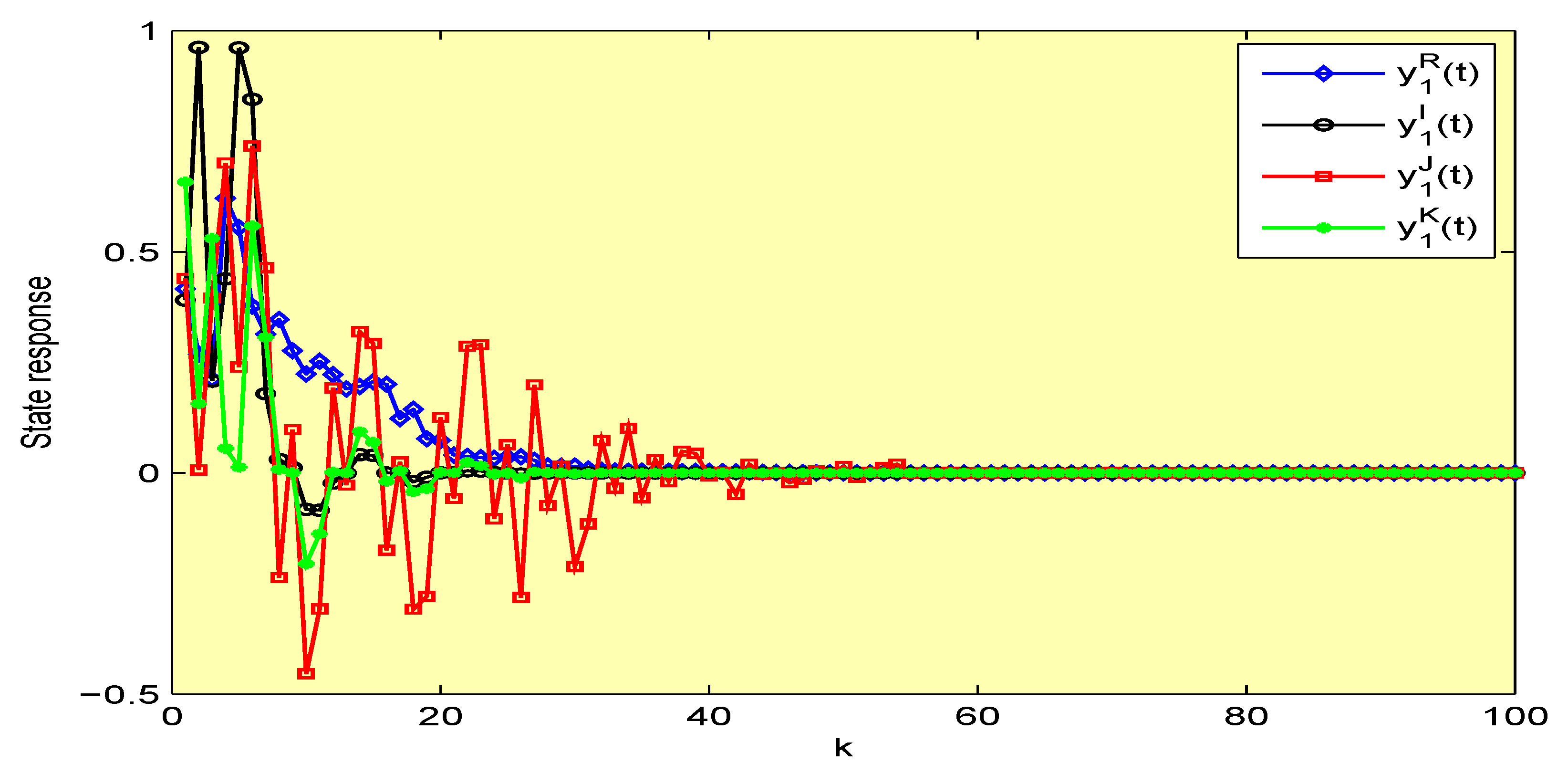
Figure 1. Results of time responses for the states y 1 R ( k ) , y 1 I ( k ) , y 1 J ( k ) , y 1 K ( k ) of the NN model (8) with σ ( k , y ( k ) ) = 0.1 y ( k ) in Example 1.
Symmetry 12 00936 g001
Figure 2. Results of the time responses for the states y 2 R ( k ) , y 2 I ( k ) , y 2 J ( k ) , y 2 K ( k ) of the NN model in (8) with σ ( k , y ( k ) ) = 0.1 y ( k ) in Example 1.
Symmetry 12 00936 g002
Figure 3. Results of the time responses for the states y 1 R ( k ) , y 1 I ( k ) , y 1 J ( k ) , y 1 K ( k ) of the NN model in (8) with σ ( k , y ( k ) ) = 0 in Example 1.
Symmetry 12 00936 g003
Figure 4. Results of the time responses for the states y 2 R ( k ) , y 2 I ( k ) , y 2 J ( k ) , y 2 K ( k ) of the NN model in (8) with σ ( k , y ( k ) ) = 0 in Example 1.
Symmetry 12 00936 g004
Figure 5. Results of the time responses for the states y 1 R ( k ) , y 1 I ( k ) of the NN model in (27) with σ R ( k , y R ( k ) ) = 0.1 y R ( k ) , σ I ( k , y I ( k ) ) = 0.1 y I ( k ) in Example 2.
Symmetry 12 00936 g005
Figure 6. Results of the time responses for the states y 2 R ( k ) , y 2 I ( k ) of the NN model in (27) with σ R ( k , y R ( k ) ) = 0.1 y R ( k ) , σ I ( k , y I ( k ) ) = 0.1 y I ( k ) in Example 2.
Symmetry 12 00936 g006
Figure 7. Results of the time responses for the states y 1 R ( k ) , y 1 I ( k ) of the NN model in (27) with σ R ( k , y R ( k ) ) = σ I ( k , y I ( k ) ) = 0 in Example 2.
Symmetry 12 00936 g007
Figure 8. Results of the time responses for the states y 2 R ( k ) , y 2 I ( k ) of the NN model in (27) with σ R ( k , y R ( k ) ) = σ I ( k , y I ( k ) ) = 0 in Example 2.
Symmetry 12 00936 g008