Statistical Inference of the Lifetime Performance Index with the Log-Logistic Distribution Based on Progressive First-Failure-Censored Data


Abstract
1. Introduction
- When k = 1, , we acquire the complete sample.
- When equations k = 1, , and are satisfied, we get type-II censoring.
- When , the progressive first-failure censoring reduces to the first-failure censoring.
- When k is equal to 1, we get a simplified form: the more familiar progressive type-II censoring.
2. The Lifetime Performance Index
3. Maximum Likelihood Estimation for
4. Confidence Intervals
4.1. Asymptotic Confidence Intervals for MLE
4.2. Asymptotic Confidence Intervals for the Log-Transformed MLE
5. Bayesian Estimation
5.1. Prior Distribution and Posterior Analysis
5.2. Asymmetric and Symmetric Loss Functions
5.3. Lindley Approximation Method
5.3.1. The Squared Error Loss Function (SELF)
5.3.2. The Linex Loss Function (LF)
5.3.3. The General Entropy Loss Function (GELF)
5.4. Monte Carlo Markov Chain Method
- Step 1:
- Initialize the values of .
- Step 2:
- Set the initial value of t to 1.
- Step 3:
- Generate from .
- Step 4:
- Generate from , using the following algorithm:
- Step 4-1:
- Generate from .
- Step 4-2:
- Generate from .
- Step 4-3:
- Set and .
- Step 5:
- t = .
- Step 6:
- Repeat steps 3–5 for M times.
6. Simulation Results
- (1)
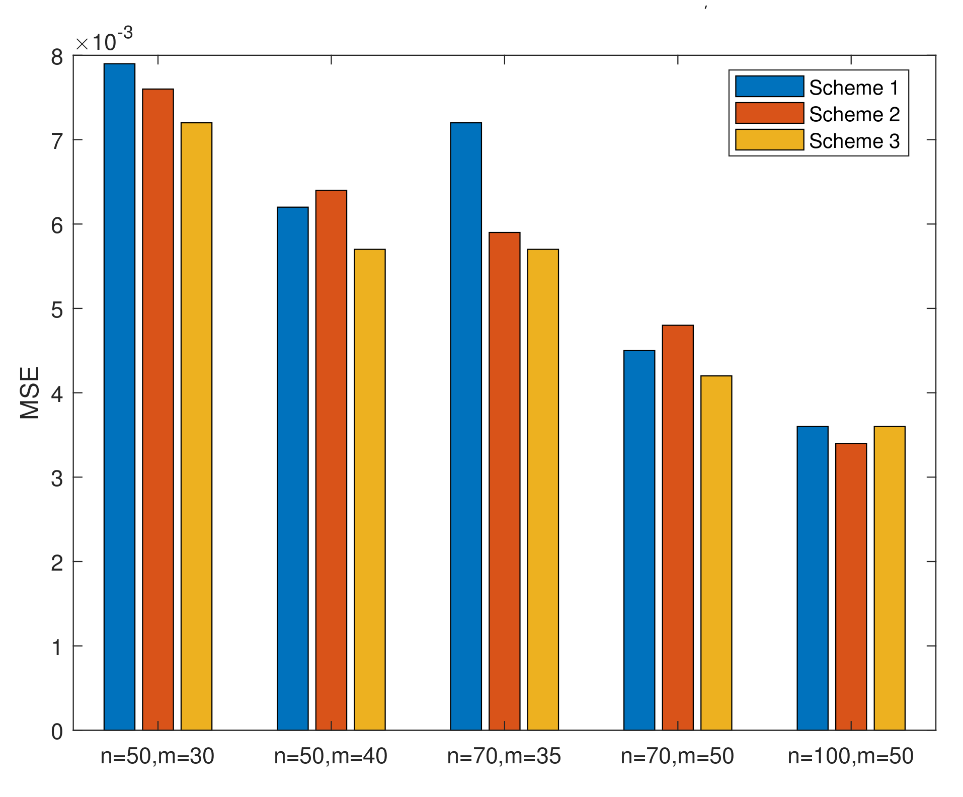
- From Table 1, we conclude that, in MLE, the MSEs of increase as k increases when n and m are invariant and decrease as n or m increases when k is invariant. The MSEs of and decrease when we assume that only one of the three parameters (k, m, and n) increases and that the other two are invariant. Figure 2 is drawn to better illustrate the relationship. In all cases, the MSEs of the parameters and the lifetime performance index perform well since the values of MSEs are close to 0.
- (2)
- From Table 2, we conclude that, in Bayesian estimation, the MSEs of , , and decrease when we assume that m or n increases and that the k is invariant. When m and n are invariant, the MSEs of increase while the MSEs of and decrease as k increases. From Table 2, Table 3, Table 4, Table 5, Table 6 and Table 7, the Bayesian estimation results based on the Lindley method perform better than the Bayesian estimation based on Metropolis–Hastings method in respect of MSEs. From Table 3 and Table 4, the result of Lindley approximation under LF when performs better than when . From Table 5 and Table 6, the result of Lindley approximation under GELF when performs better than when . It is also concluded from Table 1, Table 2, Table 3, Table 4, Table 5, Table 6 and Table 7 that the point estimation performs better as the failure proportion increases when k is invariant.
- (3)
- In Table 8, when we set that only one of the three parameters (k, m, and n) increases and the other two are invariant, the average length (AL) of 95% asymptotic confidence/HPD credible intervals narrow down. In almost all cases, the CP of reaches their prescribed confidence intervals. To conclude, it is better to apply the log-transformed MLEs than MLEs when considering the asymptotic confidence intervals.
7. Real Data Analysis
8. Optimal Censoring Plan
- Criterion 1:
- . Under this criterion, the optimal censoring scheme for the experiment is supposed to have the minimum value of the determinant of of MLEs.
- Criterion 2:
- . The optimal censoring scheme is considered to have the minimum value of the trace of of MLEs under this criterion. Without scale-invariant characteristic, criteria 1 and 2 are efficacious when lifetime distributions have one parameter.
- Criterion 3:
- . Under this criterion, the optimal censoring scheme has the minimum value of and the pth quantile of the MLE logarithmic variance of log-logistic distribution can also be written as . We can get the approximation value of as , where . The results of criterion 3 hinges on the selection of p.
- Criterion 4:
- . is defined in criterion 3. is nonnegative and satisfies . We take when .
9. Conclusions
Author Contributions
Funding
Conflicts of Interest
Appendix A. Second Derivatives of l
Appendix B. Third Derivatives of l (lij)
Appendix C. ϕi and ϕij
Appendix C.1. The Squared Error Loss Function
Appendix C.2. The Linex Loss Function
Appendix C.3. The General Entropy Loss Function
Appendix D. Complete Tables

| k | n | m | Censoring Scheme | ||||||
|---|---|---|---|---|---|---|---|---|---|
| EV | MSE | EV | MSE | EV | MSE | ||||
| 50 | 30 | (10,0*28,10) | 1.2698 | 0.0095 | 3.6439 | 0.3285 | 0.4650 | 0.0072 | |
| (1*20,0*10) | 1.2674 | 0.0104 | 3.6252 | 0.2708 | 0.4635 | 0.0072 | |||
| (1*10,0*10,1*10) | 1.2638 | 0.0099 | 3.6553 | 0.3277 | 0.4602 | 0.0073 | |||
| 40 | (10,0*39) | 1.2626 | 0.0070 | 3.6085 | 0.2183 | 0.4725 | 0.0058 | ||
| (1*10,0*30) | 1.2605 | 0.0075 | 3.6145 | 0.2165 | 0.4709 | 0.0061 | |||
| (0*39,10) | 1.2655 | 0.0075 | 3.6111 | 0.2527 | 0.4702 | 0.0058 | |||
| 70 | 35 | (35,0*34) | 1.2637 | 0.0074 | 3.6280 | 0.2480 | 0.4740 | 0.0067 | |
| 2 | (1*35) | 1.2607 | 0.0082 | 3.6466 | 0.2640 | 0.4621 | 0.0055 | ||
| (0*34,35) | 1.2661 | 0.0097 | 3.6838 | 0.3380 | 0.4576 | 0.0055 | |||
| 50 | ((0,1)*20,1*10) | 1.2572 | 0.0056 | 3.5581 | 0.1704 | 0.4651 | 0.0039 | ||
| (1*20,0*30) | 1.2629 | 0.0064 | 3.5498 | 0.1446 | 0.4701 | 0.0041 | |||
| (0*30,1*20) | 1.2632 | 0.0055 | 3.5833 | 0.1900 | 0.4717 | 0.0042 | |||
| 100 | 50 | (25,0*48,25) | 1.2623 | 0.0053 | 3.5918 | 0.1952 | 0.4706 | 0.0039 | |
| (1*50) | 1.2659 | 0.0063 | 3.5857 | 0.1817 | 0.4720 | 0.0033 | |||
| (0*49,50) | 1.2640 | 0.0063 | 3.6134 | 0.2293 | 0.4659 | 0.0031 | |||
| 50 | 30 | (10,0*28,10) | 1.2719 | 0.0104 | 3.6619 | 0.3446 | 0.4599 | 0.0059 | |
| (1*20,0*10) | 1.2733 | 0.0113 | 3.6188 | 0.2704 | 0.4624 | 0.0056 | |||
| (1*10,0*10,1*10) | 1.2672 | 0.0106 | 3.6655 | 0.3519 | 0.4566 | 0.0059 | |||
| 40 | (10,0*39) | 1.2583 | 0.0072 | 3.6025 | 0.2321 | 0.4622 | 0.0050 | ||
| (1*10,0*30) | 1.2623 | 0.0075 | 3.6073 | 0.2108 | 0.4683 | 0.0051 | |||
| (0*39,10) | 1.2681 | 0.0072 | 3.6138 | 0.2479 | 0.4676 | 0.0044 | |||
| 70 | 35 | (35,0*34) | 1.2598 | 0.0078 | 3.6254 | 0.2461 | 0.4652 | 0.0062 | |
| 3 | (1*35) | 1.2716 | 0.0102 | 3.6170 | 0.2487 | 0.4612 | 0.0052 | ||
| (0*34,35) | 1.2849 | 0.01359 | 3.6439 | 0.3340 | 0.4577 | 0.0049 | |||
| 50 | ((0,1)*20,1*10) | 1.2622 | 0.0065 | 3.5916 | 0.1788 | 0.4699 | 0.0037 | ||
| (1*20,0*30) | 1.2621 | 0.0058 | 3.5629 | 0.1571 | 0.4698 | 0.0036 | |||
| (0*30,1*20) | 1.2654 | 0.0065 | 3.5757 | 0.1893 | 0.4667 | 0.0033 | |||
| 100 | 50 | (25,0*48,25) | 1.2661 | 0.00702 | 3.5754 | 0.1912 | 0.4644 | 0.0032 | |
| (1*50) | 1.2615 | 0.0065 | 3.5773 | 0.1625 | 0.4642 | 0.0032 | |||
| (0*49,50) | 1.2732 | 0.0099 | 3.5850 | 0.2182 | 0.4597 | 0.0034 | |||
| k | n | m | Censoring Scheme | ||||||
|---|---|---|---|---|---|---|---|---|---|
| EV | MSE | EV | MSE | EV | MSE | ||||
| 50 | 30 | (10,0*28,10) | 1.2610 | 0.0081 | 3.3762 | 0.2431 | 0.4563 | 0.0067 | |
| (1*20,0*10) | 1.2555 | 0.0085 | 3.4266 | 0.1880 | 0.4595 | 0.0063 | |||
| (1*10,0*10,1*10) | 1.2526 | 0.0083 | 3.4054 | 0.2255 | 0.4523 | 0.0066 | |||
| 40 | (10,0*39) | 1.2539 | 0.0070 | 3.3997 | 0.1626 | 0.4640 | 0.0064 | ||
| (1*10,0*30) | 1.2586 | 0.0072 | 3.4048 | 0.1738 | 0.4656 | 0.0057 | |||
| (0*39,10) | 1.2548 | 0.0062 | 3.4168 | 0.1960 | 0.4625 | 0.0053 | |||
| 70 | 35 | (35,0*34) | 1.2545 | 0.0078 | 3.4026 | 0.1740 | 0.4628 | 0.0070 | |
| 2 | (1*35) | 1.2581 | 0.0081 | 3.4122 | 0.1888 | 0.4563 | 0.0051 | ||
| (0*34,35) | 1.2572 | 0.0084 | 3.4070 | 0.2300 | 0.4465 | 0.0064 | |||
| 50 | ((0,1)*20,1*10) | 1.2527 | 0.0055 | 3.4133 | 0.1301 | 0.4629 | 0.0042 | ||
| (1*20,0*30) | 1.2588 | 0.0054 | 3.4235 | 0.1313 | 0.4702 | 0.0040 | |||
| (0*30,1*20) | 1.2536 | 0.0056 | 3.4317 | 0.1467 | 0.4638 | 0.0039 | |||
| 100 | 50 | (25,0*48,25) | 1.2575 | 0.0051 | 3.4157 | 0.1479 | 0.4645 | 0.0033 | |
| (1*50) | 1.2575 | 0.0056 | 3.4257 | 0.1315 | 0.4642 | 0.0032 | |||
| (0*49,50) | 1.2557 | 0.0056 | 3.4371 | 0.1546 | 0.4593 | 0.0032 | |||
| 50 | 30 | (10,0*28,10) | 1.2608 | 0.0094 | 3.4006 | 0.2377 | 0.4496 | 0.0061 | |
| (1*20,0*10) | 1.2621 | 0.0094 | 3.4085 | 0.2194 | 0.4539 | 0.0056 | |||
| (1*10,0*10,1*10) | 1.2624 | 0.0094 | 3.3970 | 0.2268 | 0.4508 | 0.0058 | |||
| 40 | (10,0*39) | 1.2518 | 0.0072 | 3.4408 | 0.1851 | 0.4599 | 0.0055 | ||
| (1*10,0*30) | 1.2648 | 0.0068 | 3.3997 | 0.1563 | 0.4670 | 0.0046 | |||
| (0*39,10) | 1.2592 | 0.0067 | 3.4169 | 0.2072 | 0.4579 | 0.0038 | |||
| 70 | 35 | (35,0*34) | 1.2556 | 0.0072 | 3.4091 | 0.1545 | 0.4606 | 0.0053 | |
| 3 | (1*35) | 1.2636 | 0.0094 | 3.3899 | 0.1784 | 0.4517 | 0.0050 | ||
| (0*34,35) | 1.2701 | 0.0117 | 3.3897 | 0.2274 | 0.4458 | 0.0052 | |||
| 50 | ((0,1)*20,1*10) | 1.2612 | 0.0059 | 3.4059 | 0.1287 | 0.4647 | 0.0035 | ||
| (1*20,0*30) | 1.2568 | 0.0055 | 3.4389 | 0.1172 | 0.4673 | 0.0035 | |||
| (0*30,1*20) | 1.2579 | 0.0058 | 3.3978 | 0.1594 | 0.4572 | 0.0033 | |||
| 100 | 50 | (25,0*48,25) | 1.2573 | 0.0061 | 3.4185 | 0.1616 | 0.4566 | 0.0031 | |
| (1*50) | 1.2597 | 0.0066 | 3.426 | 0.1431 | 0.4599 | 0.0032 | |||
| (0*49,50) | 1.2620 | 0.0080 | 3.416 | 0.1604 | 0.4534 | 0.0033 | |||
| k | n | m | Censoring Scheme | ||||||
|---|---|---|---|---|---|---|---|---|---|
| EV | MSE | EV | MSE | EV | MSE | ||||
| 50 | 30 | (10,0*28,10) | 1.2650 | 0.0086 | 3.5013 | 0.2675 | 0.4542 | 0.0073 | |
| (1*20,0*10) | 1.2619 | 0.0096 | 3.5038 | 0.2230 | 0.4521 | 0.0075 | |||
| (1*10,0*10,1*10) | 1.2644 | 0.0085 | 3.5304 | 0.2473 | 0.4572 | 0.0065 | |||
| 40 | (10,0*39) | 1.2553 | 0.0068 | 3.5103 | 0.1761 | 0.4632 | 0.0065 | ||
| (1*10,0*30) | 1.2574 | 0.0077 | 3.4775 | 0.1740 | 0.4587 | 0.0067 | |||
| (0*39,10) | 1.2618 | 0.0064 | 3.5001 | 0.2153 | 0.4630 | 0.0058 | |||
| 70 | 35 | (35,0*34) | 1.2593 | 0.0082 | 3.5016 | 0.1950 | 0.4598 | 0.0070 | |
| 2 | (1*35) | 1.2602 | 0.0081 | 3.5187 | 0.2008 | 0.4540 | 0.0052 | ||
| (0*34,35) | 1.2739 | 0.0095 | 3.5054 | 0.2496 | 0.4534 | 0.0054 | |||
| 50 | ((0,1)*20,1*10) | 1.2596 | 0.0055 | 3.4922 | 0.1518 | 0.4649 | 0.0039 | ||
| (1*20,0*30) | 1.2574 | 0.0059 | 3.4804 | 0.1226 | 0.4636 | 0.0043 | |||
| (0*30,1*20) | 1.2587 | 0.0055 | 3.4952 | 0.1588 | 0.4639 | 0.0041 | |||
| 100 | 50 | (25,0*48,25) | 1.2539 | 0.0049 | 3.5156 | 0.1729 | 0.4601 | 0.0039 | |
| (1*50) | 1.2610 | 0.0057 | 3.4682 | 0.1379 | 0.4603 | 0.0037 | |||
| (0*49,50) | 1.2616 | 0.0071 | 3.5032 | 0.1918 | 0.4546 | 0.0038 | |||
| 50 | 30 | (10,0*28,10) | 1.2654 | 0.0102 | 3.5405 | 0.2759 | 0.4491 | 0.0067 | |
| (1*20,0*10) | 1.2690 | 0.0104 | 3.5134 | 0.2123 | 0.4538 | 0.0064 | |||
| (1*10,0*10,1*10) | 1.2642 | 0.0104 | 3.5086 | 0.2310 | 0.4459 | 0.0066 | |||
| 40 | (10,0*39) | 1.2551 | 0.0068 | 3.5144 | 0.1702 | 0.4587 | 0.0050 | ||
| (1*10,0*30) | 1.2569 | 0.0066 | 3.5013 | 0.1836 | 0.4572 | 0.0051 | |||
| (0*39,10) | 1.2620 | 0.0068 | 3.4972 | 0.2024 | 0.4558 | 0.0045 | |||
| 70 | 35 | (35,0*34) | 1.2624 | 0.0081 | 3.4915 | 0.1846 | 0.4583 | 0.0057 | |
| 3 | (1*35) | 1.2673 | 0.0104 | 3.5076 | 0.2120 | 0.4494 | 0.0052 | ||
| (0*34,35) | 1.2774 | 0.0123 | 3.5015 | 0.2466 | 0.4428 | 0.0055 | |||
| 50 | ((0,1)*20,1*10) | 1.2582 | 0.0059 | 3.4849 | 0.1467 | 0.4586 | 0.0036 | ||
| (1*20,0*30) | 1.2585 | 0.0055 | 3.5161 | 0.1315 | 0.4664 | 0.0036 | |||
| (0*30,1*20) | 1.2600 | 0.0067 | 3.5050 | 0.1851 | 0.4570 | 0.0036 | |||
| 100 | 50 | (25,0*48,25) | 1.2644 | 0.0068 | 3.4909 | 0.1482 | 0.4591 | 0.0033 | |
| (1*50) | 1.2623 | 0.0070 | 3.5024 | 0.1658 | 0.4575 | 0.0034 | |||
| (0*49,50) | 1.2663 | 0.0082 | 3.5159 | 0.1780 | 0.4534 | 0.0036 | |||
| k | n | m | Censoring Scheme | ||||||
|---|---|---|---|---|---|---|---|---|---|
| EV | MSE | EV | MSE | EV | MSE | ||||
| 50 | 30 | (10,0*28,10) | 1.2097 | 0.0065 | 2.6748 | 0.6893 | 0.5273 | 0.0083 | |
| (1*20,0*10) | 1.2086 | 0.0071 | 2.7004 | 0.6471 | 0.5291 | 0.0091 | |||
| (1*10,0*10,1*10) | 1.2098 | 0.0069 | 2.6863 | 0.6661 | 0.5281 | 0.0089 | |||
| 40 | (10,0*39) | 1.2006 | 0.0060 | 2.6951 | 0.6388 | 0.5351 | 0.0086 | ||
| (1*10,0*30) | 1.2024 | 0.0062 | 2.7056 | 0.6257 | 0.5370 | 0.0088 | |||
| (0*39,10) | 1.2061 | 0.0054 | 2.6908 | 0.6571 | 0.5376 | 0.0085 | |||
| 70 | 35 | (35,0*34) | 1.2041 | 0.0065 | 2.6854 | 0.6556 | 0.5324 | 0.0087 | |
| 2 | (1*35) | 1.2097 | 0.0062 | 2.6992 | 0.6482 | 0.5310 | 0.0076 | ||
| (0*34,35) | 1.2138 | 0.0064 | 2.6912 | 0.6637 | 0.5257 | 0.0073 | |||
| 50 | ((0,1)*20,1*10) | 1.2049 | 0.0052 | 2.6973 | 0.6228 | 0.5410 | 0.0076 | ||
| (1*20,0*30) | 1.2023 | 0.0056 | 2.6907 | 0.6329 | 0.5370 | 0.0073 | |||
| (0*30,1*20) | 1.2015 | 0.0054 | 2.7052 | 0.6213 | 0.5374 | 0.0073 | |||
| 100 | 50 | (25,0*48,25) | 1.2044 | 0.0050 | 2.6879 | 0.6447 | 0.5358 | 0.0067 | |
| (1*50) | 1.2028 | 0.0055 | 2.7009 | 0.6240 | 0.5342 | 0.0063 | |||
| (0*49,50) | 1.2042 | 0.0059 | 2.7025 | 0.6282 | 0.5295 | 0.0060 | |||
| 50 | 30 | (10,0*28,10) | 1.2179 | 0.0064 | 2.6892 | 0.6642 | 0.5294 | 0.0077 | |
| (1*20,0*10) | 1.2083 | 0.0075 | 2.7018 | 0.6383 | 0.5231 | 0.0077 | |||
| (1*10,0*10,1*10) | 1.2143 | 0.0074 | 2.6812 | 0.6776 | 0.5210 | 0.0069 | |||
| 40 | (10,0*39) | 1.2034 | 0.0062 | 2.6922 | 0.6479 | 0.5310 | 0.0073 | ||
| (1*10,0*30) | 1.2086 | 0.0057 | 2.6930 | 0.6412 | 0.5356 | 0.0074 | |||
| (0*39,10) | 1.2073 | 0.0063 | 2.6806 | 0.6728 | 0.5261 | 0.0061 | |||
| 70 | 35 | (35,0*34) | 1.2030 | 0.0063 | 2.6958 | 0.6396 | 0.5289 | 0.0074 | |
| 3 | (1*35) | 1.2120 | 0.0071 | 2.6965 | 0.6438 | 0.5243 | 0.0062 | ||
| (0*34,35) | 1.2194 | 0.0075 | 2.6895 | 0.6633 | 0.5171 | 0.0062 | |||
| 50 | ((0,1)*20,1*10) | 1.2046 | 0.0053 | 2.7011 | 0.6161 | 0.5374 | 0.0066 | ||
| (1*20,0*30) | 1.2042 | 0.0054 | 2.6985 | 0.6184 | 0.5376 | 0.0066 | |||
| (0*30,1*20) | 1.2077 | 0.0051 | 2.6920 | 0.6361 | 0.5351 | 0.0061 | |||
| 100 | 50 | (25,0*48,25) | 1.2055 | 0.0055 | 2.7053 | 0.6235 | 0.5320 | 0.0059 | |
| (1*50) | 1.2098 | 0.0053 | 2.6885 | 0.6387 | 0.5342 | 0.0060 | |||
| (0*49,50) | 1.2139 | 0.0061 | 2.6811 | 0.6628 | 0.5247 | 0.0052 | |||
| k | n | m | Censoring Scheme | ||||||
|---|---|---|---|---|---|---|---|---|---|
| EV | MSE | EV | MSE | EV | MSE | ||||
| 50 | 30 | (10,0*28,10) | 1.2654 | 0.0113 | 3.5899 | 0.3877 | 0.4715 | 0.0089 | |
| (1*20,0*10) | 1.2717 | 0.0123 | 3.5746 | 0.2959 | 0.4750 | 0.0083 | |||
| (1*10,0*10,1*10) | 1.2596 | 0.0133 | 3.6023 | 0.3287 | 0.4668 | 0.0101 | |||
| 40 | (10,0*39) | 1.2666 | 0.0114 | 3.5591 | 0.2993 | 0.4761 | 0.0091 | ||
| (1*10,0*30) | 1.2523 | 0.0093 | 3.6125 | 0.3101 | 0.4714 | 0.0079 | |||
| (0*39,10) | 1.2668 | 0.0100 | 3.5813 | 0.2786 | 0.4783 | 0.0063 | |||
| 70 | 35 | (35,0*34) | 1.2578 | 0.0123 | 3.5666 | 0.2794 | 0.4681 | 0.0102 | |
| 2 | (1*35) | 1.2606 | 0.0103 | 3.5886 | 0.3060 | 0.4669 | 0.0062 | ||
| (0*34,35) | 1.2772 | 0.0136 | 3.5638 | 0.3636 | 0.4672 | 0.0063 | |||
| 50 | ((0,1)*20,1*10) | 1.2545 | 0.0081 | 3.5743 | 0.2166 | 0.4730 | 0.0062 | ||
| (1*20,0*30) | 1.2616 | 0.0075 | 3.5689 | 0.2004 | 0.4793 | 0.0057 | |||
| (0*30,1*20) | 1.2569 | 0.0075 | 3.5707 | 0.2447 | 0.4733 | 0.0056 | |||
| 100 | 50 | (25,0*48,25) | 1.2688 | 0.0084 | 3.5109 | 0.2082 | 0.4742 | 0.0054 | |
| (1*50) | 1.2584 | 0.0077 | 3.5934 | 0.2405 | 0.4734 | 0.0044 | |||
| (0*49,50) | 1.2674 | 0.0090 | 3.5566 | 0.2305 | 0.4723 | 0.0039 | |||
| 50 | 30 | (10,0*28,10) | 1.2788 | 0.0139 | 3.5777 | 0.3462 | 0.4731 | 0.0066 | |
| (1*20,0*10) | 1.2747 | 0.0150 | 3.5818 | 0.2870 | 0.4725 | 0.0072 | |||
| (1*10,0*10,1*10) | 1.2737 | 0.0146 | 3.5694 | 0.3354 | 0.4651 | 0.0069 | |||
| 40 | (10,0*39) | 1.2636 | 0.0104 | 3.5797 | 0.2753 | 0.4725 | 0.0064 | ||
| (1*10,0*30) | 1.2581 | 0.0095 | 3.6285 | 0.3061 | 0.4742 | 0.0072 | |||
| (0*39,10) | 1.2705 | 0.0112 | 3.5569 | 0.2895 | 0.4715 | 0.0060 | |||
| 70 | 35 | (35,0*34) | 1.2684 | 0.0104 | 3.5995 | 0.2798 | 0.4807 | 0.0073 | |
| 3 | (1*35) | 1.2739 | 0.0147 | 3.5713 | 0.2652 | 0.4678 | 0.0060 | ||
| (0*34,35) | 1.2999 | 0.0206 | 3.5305 | 0.3439 | 0.4690 | 0.0057 | |||
| 50 | ((0,1)*20,1*10) | 1.2575 | 0.0083 | 3.5933 | 0.2302 | 0.4723 | 0.0046 | ||
| (1*20,0*30) | 1.2551 | 0.0085 | 3.6030 | 0.2046 | 0.4731 | 0.0052 | |||
| (0*30,1*20) | 1.2690 | 0.0097 | 3.5733 | 0.2535 | 0.4754 | 0.0039 | |||
| 100 | 50 | (25,0*48,25) | 1.2729 | 0.0104 | 3.5749 | 0.2337 | 0.4773 | 0.0037 | |
| (1*50) | 1.2627 | 0.0090 | 3.6119 | 0.2165 | 0.4771 | 0.0044 | |||
| (0*49,50) | 1.2723 | 0.0125 | 3.6293 | 0.2923 | 0.4733 | 0.0038 | |||
| k | n | m | Censoring Scheme | ||||||
|---|---|---|---|---|---|---|---|---|---|
| AL | CP | AL | CP | AL | CP | ||||
| 50 | 30 | (10,0*28,10) | 0.3259 | 0.950 | 0.3422 | 0.966 | 0.3346 | 0.950 | |
| (1*20,0*10) | 0.3271 | 0.956 | 0.3364 | 0.962 | 0.3337 | 0.950 | |||
| (1*10,0*10,1*10) | 0.3210 | 0.980 | 0.3303 | 0.978 | 0.3253 | 0.974 | |||
| 40 | (10,0*39) | 0.3108 | 0.942 | 0.3171 | 0.966 | 0.3138 | 0.940 | ||
| (1*10,0*30) | 0.3037 | 0.946 | 0.3097 | 0.950 | 0.3053 | 0.924 | |||
| (0*39,10) | 0.2859 | 0.960 | 0.2908 | 0.970 | 0.2920 | 0.960 | |||
| 70 | 35 | (35,0*34) | 0.3282 | 0.960 | 0.3359 | 0.968 | 0.3318 | 0.944 | |
| 2 | (1*35) | 0.2852 | 0.976 | 0.2911 | 0.978 | 0.2897 | 0.960 | ||
| (0*34,35) | 0.2832 | 0.972 | 0.2924 | 0.988 | 0.2909 | 0.934 | |||
| 50 | ((0,1)*20,1*10) | 0.2505 | 0.952 | 0.2537 | 0.964 | 0.2532 | 0.936 | ||
| (1*20,0*30) | 0.2588 | 0.962 | 0.2624 | 0.964 | 0.2619 | 0.960 | |||
| (0*30,1*20) | 0.2426 | 0.964 | 0.2456 | 0.976 | 0.2465 | 0.950 | |||
| 100 | 50 | (25,0*48,25) | 0.2339 | 0.954 | 0.2366 | 0.974 | 0.2375 | 0.944 | |
| (1*50) | 0.2291 | 0.968 | 0.2321 | 0.984 | 0.2329 | 0.950 | |||
| (0*49,50) | 0.2266 | 0.958 | 0.2299 | 0.964 | 0.2339 | 0.946 | |||
| 50 | 30 | (10,0*28,10) | 0.2750 | 0.972 | 0.2796 | 0.980 | 0.2790 | 0.952 | |
| (1*20,0*10) | 0.2713 | 0.948 | 0.2780 | 0.950 | 0.2754 | 0.934 | |||
| (1*10,0*10,1*10) | 0.2559 | 0.954 | 0.2601 | 0.964 | 0.2648 | 0.940 | |||
| 40 | (10,0*39) | 0.2739 | 0.960 | 0.2785 | 0.970 | 0.2777 | 0.950 | ||
| (1*10,0*30) | 0.2708 | 0.952 | 0.2757 | 0.970 | 0.2743 | 0.934 | |||
| (0*39,10) | 0.2616 | 0.940 | 0.2666 | 0.964 | 0.2676 | 0.928 | |||
| 70 | 35 | (35,0*34) | 0.2921 | 0.956 | 0.2982 | 0.960 | 0.2967 | 0.932 | |
| 3 | (1*35) | 0.2779 | 0.970 | 0.2857 | 0.974 | 0.2816 | 0.942 | ||
| (0*34,35) | 0.2942 | 0.992 | 0.3098 | 0.990 | 0.3004 | 0.948 | |||
| 50 | ((0,1)*20,1*10) | 0.2315 | 0.958 | 0.2345 | 0.976 | 0.2330 | 0.948 | ||
| (1*20,0*30) | 0.2350 | 0.962 | 0.2379 | 0.964 | 0.2359 | 0.950 | |||
| (0*30,1*20) | 0.2259 | 0.960 | 0.2290 | 0.984 | 0.2293 | 0.948 | |||
| 100 | 50 | (25,0*48,25) | 0.2233 | 0.982 | 0.2262 | 0.980 | 0.2274 | 0.962 | |
| (1*50) | 0.2250 | 0.962 | 0.2301 | 0.988 | 0.2259 | 0.946 | |||
| (0*49,50) | 0.2364 | 0.968 | 0.2481 | 0.982 | 0.2365 | 0.938 |
References
- Cooper, T. Longer Lasting Products: Alternatives to the Throwaway Society; CRC Press: Boca Raton, FL, USA, 2016. [Google Scholar]
- Ertz, M.; Leblanc-Proulx, S.; Sarigllü, E.; Morin, V. Advancing quantitative rigor in the circular economy literature: New methodology for product lifetime extension business models. Resour. Conserv. Recycl. 2019, 150, 1–12. [Google Scholar] [CrossRef]
- Montgomery, D.C. Introduction to Statistical Quality Control; John Wiley & Sons: Hoboken, NJ, USA, 1991. [Google Scholar]
- Wu, J.W.; Lee, H.M.; Lei, C.L. Computational testing algorithmic procedure of assessment for lifetime performance index of products with two-parameter exponential distribution. Appl. Math. Comput. 2007, 190, 116–125. [Google Scholar] [CrossRef]
- Lee, W.C.; Wu, J.W.; Hong, C.W. Assessing the Lifetime Performance Index of Products with the Exponential Distribution under Progressively Type II Right Censored Samples; Elsevier Science: Amsterdam, The Netherlands, 2009. [Google Scholar]
- Lee, H.M.; Wu, J.W.; Lei, C.L.; Hung, W.L. Implementing lifetime performance index of products with two-parameter exponential distribution. Int. J. Syst. Sci. 2011, 42, 1305–1321. [Google Scholar] [CrossRef]
- Sultan, K.; Alsadat, N.; Kundu, D. Bayesian and maximum likelihood estimations of the inverse Weibull parameters under progressive type-II censoring. J. Stat. Comput. Simul. 2014, 84, 2248–2265. [Google Scholar] [CrossRef]
- Lee, K.; Cho, Y. Bayesian and maximum likelihood estimations of the inverted exponentiated half logistic distribution under progressive Type II censoring. J. Appl. Stat. 2016, 44, 811–832. [Google Scholar] [CrossRef]
- Cohen, A.C. Progressively Censored Samples in Life Testing. Technometrics 1963, 5, 327–339. [Google Scholar] [CrossRef]
- Mohammed, H.S. Statistical inferences based on an adaptive progressive type-II censoring from exponentiated exponential distribution. J. Egypt. Math. Soc. 2017, 25, 393–399. [Google Scholar]
- Balakrishnan, N.; Aggarwala, R. Progressive Censoring: Theory, Methods, and Applications; Birkhäuser: Boston, MA, USA, 2000. [Google Scholar]
- Johnson, L.G. Theory And Technique Of Variation Research; Elsevier Pub. Co.: Amsterdam, The Netherlands, 1964. [Google Scholar]
- Wu, S.J.; Kuş, C. On estimation based on progressive first-failure-censored sampling. Comput. Stat. Data Anal. 2009, 53, 3659–3670. [Google Scholar] [CrossRef]
- Ahmed, E.A. Estimation and prediction for the generalized inverted exponential distribution based on progressively first-failure-censored data with application. J. Appl. Stat. 2017, 44, 1576–1608. [Google Scholar] [CrossRef]
- Madhulika, D.; Renu, G.; Hare, K. On progressively first failure censored Lindley distribution. Comput. Stat. 2016, 31, 139–163. [Google Scholar]
- Soliman, A.A.; Abd-Ellah, A.H.; Abou-Elheggag, N.A.; Abd-Elmougod, G.A. Estimation of the parameters of life for Gompertz distribution using progressive first-failure censored data. Comput. Stat. Data Anal. 2012, 56, 2471–2485. [Google Scholar] [CrossRef]
- Ahmadi, M.V.; Doostparast, M.; Ahmadi, J. Estimating the lifetime performance index with Weibull distribution based on progressive first-failure censoring scheme. J. Comput. Appl. Math. 2013, 239, 93–102. [Google Scholar] [CrossRef]
- Madhulika, D.; Hare, K.; Renu, G. Generalized inverted exponential distribution under progressive first-failure censoring. J. Stat. Comput. Simul. 2016, 86, 1095–1114. [Google Scholar]
- Ahmed, A.; Soliman, M.M.A.S. Bayesian MCMC inference for the Gompertz distribution based on progressive first-failure censoring data. AIP Conf. Proc. 2015, 1643, 125–134. [Google Scholar]
- Ahmadi, M.V.; Doostparast, M. Pareto analysis for the lifetime performance index of products on the basis of progressively first-failure-censored batches under balanced symmetric and asymmetric loss functions. J. Appl. Stat. 2019, 46, 1196–1227. [Google Scholar] [CrossRef]
- Akhtar, M.T.; Khan, A.A.; Akhtar, M.T.; Khan, A.A. Log-logistic Distribution as a Reliability Model: A Bayesian Analysis. Am. J. Math. Stat. 2014, 4, 162–170. [Google Scholar]
- Al-Shomrani, A.A.; Shawky, A.I.; Arif, O.H.; Aslam, M. Log-logistic distribution for survival data analysis using MCMC. Springerplus 2016, 5, 1774. [Google Scholar] [CrossRef]
- Lesitha, G.P.Y.T. Estimation of the scale parameter of a log-logistic distribution. Metrika 2013, 76, 427–448. [Google Scholar] [CrossRef]
- William, Q.; Meeker; Luis, A. Escobar Statistical Methods for Reliability Data. Technometrics 1998, 40, 254–256. [Google Scholar]
- Lindley, D.V. Approximate Bayesian methods. Trab. Estad. Y Investig. Oper. 1980, 31, 223–245. [Google Scholar] [CrossRef]
- Nassar, M.; Abo-Kasem, O.; Zhang, C.; Dey, S. Analysis of Weibull Distribution Under Adaptive Type-II Progressive Hybrid Censoring Scheme. J. Ind. Soc. Probab. Stat. 2018, 19, 25–65. [Google Scholar] [CrossRef]
- Albert, J.; Chopin, N. Bayesian computation with R. Stat. Comput. 2009, 19, 111–112. [Google Scholar]
- Balakrishnan, N.; Sandhu, R.A. A Simple Simulational Algorithm for Generating Progressive Type-II Censored Samples. Am. Stat. 1995, 49, 229–230. [Google Scholar]
- Nichols, M.D.; Padgett, W.J. A Bootstrap Control Chart for Weibull Percentiles. Qual. Reliab. Eng. 2006, 22, 141–151. [Google Scholar] [CrossRef]
- Mohammed, H.S.; Ateya, S.F.; AL-Hussaini, E.K. Estimation based on progressive first-failure censoring from exponentiated exponential distribution. J. Appl. Stat. 2017, 44, 1479–1494. [Google Scholar] [CrossRef]
- Pradhan, B.; Kundu, D. On progressively censored generalized exponential distribution. Test 2009, 18, 497–515. [Google Scholar] [CrossRef]
- Den Hollander, M.C.; Bakker, C.A.; Hultink, E.J. Product Design in a Circular Economy: Development of a Typology of Key Concepts and Terms. J. Ind. Ecol. 2017, 21, 517–525. [Google Scholar] [CrossRef]
- Ertz, M.; Leblanc-Proulx, S.; Sarigollu, E.; Morin, V. Made to break? A taxonomy of business models on product lifetime extension. J. Clean. Prod. 2019, 234, 867–880. [Google Scholar] [CrossRef]


| k | n | m | Censoring Scheme | ||||||
|---|---|---|---|---|---|---|---|---|---|
| EV | MSE | EV | MSE | EV | MSE | ||||
| 50 | 30 | (10,0*28,10) | 1.2440 | 0.0091 | 3.6203 | 0.3579 | 0.4656 | 0.0079 | |
| (1*20,0*10) | 1.2414 | 0.0098 | 3.6027 | 0.3014 | 0.4620 | 0.0076 | |||
| (1*10,0*10,1*10) | 1.2369 | 0.0087 | 3.6118 | 0.3305 | 0.4593 | 0.0072 | |||
| 40 | (10,0*39) | 1.2476 | 0.0068 | 3.5585 | 0.2127 | 0.4730 | 0.0062 | ||
| (1*10,0*30) | 1.2480 | 0.0073 | 3.5454 | 0.2145 | 0.4707 | 0.0064 | |||
| (0*39,10) | 1.2440 | 0.0065 | 3.6012 | 0.2883 | 0.4704 | 0.0057 | |||
| 70 | 35 | (35,0*34) | 1.2448 | 0.0081 | 3.5508 | 0.2503 | 0.4659 | 0.0072 | |
| 2 | (1*35) | 1.2453 | 0.0083 | 3.5879 | 0.2641 | 0.4654 | 0.0059 | ||
| (0*34,35) | 1.2448 | 0.0089 | 3.6055 | 0.3615 | 0.4606 | 0.0057 | |||
| 50 | ((0,1)*20,1*10) | 1.2477 | 0.0056 | 3.5354 | 0.1625 | 0.4716 | 0.0045 | ||
| (1*20,0*30) | 1.2472 | 0.0062 | 3.5310 | 0.1531 | 0.4705 | 0.0048 | |||
| (0*30,1*20) | 1.2443 | 0.0057 | 3.5573 | 0.1998 | 0.4684 | 0.0042 | |||
| 100 | 50 | (25,0*48,25) | 1.2472 | 0.0058 | 3.5471 | 0.2007 | 0.4685 | 0.0036 | |
| (1*50) | 1.2452 | 0.0053 | 3.5579 | 0.1829 | 0.4690 | 0.0034 | |||
| (0*49,50) | 1.2395 | 0.0065 | 3.5943 | 0.2395 | 0.4636 | 0.0036 | |||
| 50 | 30 | (10,0*28,10) | 1.2360 | 0.0098 | 3.6429 | 0.3770 | 0.4558 | 0.0066 | |
| (1*20,0*10) | 1.2442 | 0.0095 | 3.5869 | 0.2668 | 0.4632 | 0.0063 | |||
| (1*10,0*10,1*10) | 1.2398 | 0.0104 | 3.6182 | 0.3441 | 0.4565 | 0.0066 | |||
| 40 | (10,0*39) | 1.2423 | 0.0070 | 3.5580 | 0.2206 | 0.4648 | 0.0054 | ||
| (1*10,0*30) | 1.2458 | 0.0069 | 3.5482 | 0.1808 | 0.4679 | 0.0048 | |||
| (0*39,10) | 1.2423 | 0.0073 | 3.5772 | 0.2633 | 0.4630 | 0.0047 | |||
| 70 | 35 | (35,0*34) | 1.2428 | 0.0077 | 3.5670 | 0.2448 | 0.4647 | 0.0057 | |
| 3 | (1*35) | 1.2385 | 0.0096 | 3.6074 | 0.2744 | 0.4566 | 0.0055 | ||
| (0*34,35) | 1.2367 | 0.0133 | 3.6284 | 0.3616 | 0.4457 | 0.0071 | |||
| 50 | ((0,1)*20,1*10) | 1.2421 | 0.0061 | 3.5498 | 0.1640 | 0.4651 | 0.0037 | ||
| (1*20,0*30) | 1.2494 | 0.0063 | 3.5304 | 0.1549 | 0.4705 | 0.0041 | |||
| (0*30,1*20) | 1.2384 | 0.0059 | 3.5876 | 0.2118 | 0.4635 | 0.0034 | |||
| 100 | 50 | (25,0*48,25) | 1.2405 | 0.0069 | 3.5650 | 0.2184 | 0.4596 | 0.0038 | |
| (1*50) | 1.2402 | 0.0070 | 3.5460 | 0.1738 | 0.4590 | 0.0039 | |||
| (0*49,50) | 1.2412 | 0.0080 | 3.5678 | 0.2286 | 0.4572 | 0.0037 | |||
| k | n | m | Censoring Scheme | ||||||
|---|---|---|---|---|---|---|---|---|---|
| EV | MSE | EV | MSE | EV | MSE | ||||
| 50 | 30 | (10,0*28,10) | 1.2651 | 0.0089 | 3.4924 | 0.2412 | 0.5715 | 0.0200 | |
| (1*20,0*10) | 1.2595 | 0.0098 | 3.5247 | 0.2380 | 0.5595 | 0.0172 | |||
| (1*10,0*10,1*10) | 1.2625 | 0.0095 | 3.5065 | 0.2421 | 0.5653 | 0.0185 | |||
| 40 | (10,0*39) | 1.2534 | 0.0069 | 3.5171 | 0.1754 | 0.5369 | 0.0117 | ||
| (1*10,0*30) | 1.2606 | 0.0078 | 3.5059 | 0.2048 | 0.5379 | 0.0118 | |||
| (0*39,10) | 1.2616 | 0.0066 | 3.5034 | 0.2006 | 0.5503 | 0.0132 | |||
| 70 | 35 | (35,0*34) | 1.2643 | 0.0079 | 3.5023 | 0.1841 | 0.5488 | 0.0147 | |
| 2 | (1*35) | 1.2620 | 0.0087 | 3.5125 | 0.2079 | 0.5531 | 0.0126 | ||
| (0*34,35) | 1.2643 | 0.0090 | 3.5226 | 0.2464 | 0.5802 | 0.0183 | |||
| 50 | ((0,1)*20,1*10) | 1.2548 | 0.0056 | 3.5019 | 0.1464 | 0.5264 | 0.0081 | ||
| (1*20,0*30) | 1.2558 | 0.0051 | 3.4950 | 0.1297 | 0.5236 | 0.0070 | |||
| (0*30,1*20) | 1.2572 | 0.0052 | 3.5059 | 0.1623 | 0.5343 | 0.0083 | |||
| 100 | 50 | (25,0*48,25) | 1.2564 | 0.0049 | 3.4998 | 0.1655 | 0.5326 | 0.0076 | |
| (1*50) | 1.2571 | 0.0059 | 3.5092 | 0.1494 | 0.5288 | 0.0070 | |||
| (0*49,50) | 1.2623 | 0.0061 | 3.5018 | 0.1799 | 0.5470 | 0.0088 | |||
| 50 | 30 | (10,0*28,10) | 1.2658 | 0.0102 | 3.5151 | 0.2710 | 0.5765 | 0.0182 | |
| (1*20,0*10) | 1.2629 | 0.0099 | 3.5083 | 0.2272 | 0.5578 | 0.0145 | |||
| (1*10,0*10,1*10) | 1.2668 | 0.0107 | 3.5254 | 0.2623 | 0.5735 | 0.0179 | |||
| 40 | (10,0*39) | 1.2583 | 0.0069 | 3.5051 | 0.1790 | 0.5390 | 0.0103 | ||
| (1*10,0*30) | 1.258 | 0.0068 | 3.488 | 0.1671 | 0.5350 | 0.0097 | |||
| (0*39,10) | 1.2586 | 0.0068 | 3.5219 | 0.1944 | 0.5530 | 0.0120 | |||
| 70 | 35 | (35,0*34) | 1.2610 | 0.0082 | 3.5065 | 0.2021 | 0.5427 | 0.0117 | |
| 3 | (1*35) | 1.2676 | 0.0101 | 3.5050 | 0.2141 | 0.5575 | 0.0124 | ||
| (0*34,35) | 1.2752 | 0.0135 | 3.5142 | 0.2524 | 0.5891 | 0.0186 | |||
| 50 | ((0,1)*20,1*10) | 1.2630 | 0.0061 | 3.4780 | 0.1449 | 0.5283 | 0.0069 | ||
| (1*20,0*30) | 1.2588 | 0.0057 | 3.5038 | 0.1233 | 0.5257 | 0.0064 | |||
| (0*30,1*20) | 1.2639 | 0.0062 | 3.4899 | 0.1593 | 0.5377 | 0.0075 | |||
| 100 | 50 | (25,0*48,25) | 1.2632 | 0.0065 | 3.4992 | 0.1443 | 0.5412 | 0.0080 | |
| (1*50) | 1.2628 | 0.0065 | 3.4840 | 0.1516 | 0.5302 | 0.0063 | |||
| (0*49,50) | 1.2667 | 0.0081 | 3.4991 | 0.1852 | 0.5521 | 0.0091 | |||
| k | n | m | Censoring Scheme | ||||||
|---|---|---|---|---|---|---|---|---|---|
| EV | MSE | EV | MSE | EV | MSE | ||||
| 50 | 30 | (10,0*28,10) | 1.2698 | 0.0095 | 3.6439 | 0.3285 | 0.4650 | 0.0072 | |
| (1*20,0*10) | 1.2674 | 0.0104 | 3.6252 | 0.2708 | 0.4635 | 0.0072 | |||
| (1*10,0*10,1*10) | 1.2638 | 0.0099 | 3.6553 | 0.3277 | 0.4602 | 0.0073 | |||
| 40 | (10,0*39) | 1.2626 | 0.0070 | 3.6085 | 0.2183 | 0.4725 | 0.0058 | ||
| (1*10,0*30) | 1.2605 | 0.0075 | 3.6145 | 0.2165 | 0.4709 | 0.0061 | |||
| (0*39,10) | 1.2655 | 0.0075 | 3.6111 | 0.2527 | 0.4702 | 0.0058 | |||
| 70 | 35 | (35,0*34) | 1.2637 | 0.0074 | 3.6280 | 0.2480 | 0.4740 | 0.0067 | |
| 2 | (1*35) | 1.2607 | 0.0082 | 3.6466 | 0.2640 | 0.4621 | 0.0055 | ||
| (0*34,35) | 1.2661 | 0.0097 | 3.6838 | 0.3380 | 0.4576 | 0.0055 | |||
| 50 | ((0,1)*20,1*10) | 1.2572 | 0.0056 | 3.5581 | 0.1704 | 0.4651 | 0.0039 | ||
| (1*20,0*30) | 1.2629 | 0.0064 | 3.5498 | 0.1446 | 0.4701 | 0.0041 | |||
| (0*30,1*20) | 1.2632 | 0.0055 | 3.5833 | 0.1900 | 0.4717 | 0.0042 | |||
| 100 | 50 | (25,0*48,25) | 1.2623 | 0.0053 | 3.5918 | 0.1952 | 0.4706 | 0.0039 | |
| (1*50) | 1.2659 | 0.0063 | 3.5857 | 0.1817 | 0.4720 | 0.0033 | |||
| (0*49,50) | 1.2640 | 0.0063 | 3.6134 | 0.2293 | 0.4659 | 0.0031 | |||
| k | n | m | Censoring Scheme | ||||||
|---|---|---|---|---|---|---|---|---|---|
| EV | MSE | EV | MSE | EV | MSE | ||||
| 50 | 30 | (10,0*28,10) | 1.2610 | 0.0081 | 3.3762 | 0.2431 | 0.4563 | 0.0067 | |
| (1*20,0*10) | 1.2555 | 0.0085 | 3.4266 | 0.1880 | 0.4595 | 0.0063 | |||
| (1*10,0*10,1*10) | 1.2526 | 0.0083 | 3.4054 | 0.2255 | 0.4523 | 0.0066 | |||
| 40 | (10,0*39) | 1.2539 | 0.0070 | 3.3997 | 0.1626 | 0.4640 | 0.0064 | ||
| (1*10,0*30) | 1.2586 | 0.0072 | 3.4048 | 0.1738 | 0.4656 | 0.0057 | |||
| (0*39,10) | 1.2548 | 0.0062 | 3.4168 | 0.1960 | 0.4625 | 0.0053 | |||
| 70 | 35 | (35,0*34) | 1.2545 | 0.0078 | 3.4026 | 0.1740 | 0.4628 | 0.0070 | |
| 2 | (1*35) | 1.2581 | 0.0081 | 3.4122 | 0.1888 | 0.4563 | 0.0051 | ||
| (0*34,35) | 1.2572 | 0.0084 | 3.4070 | 0.2300 | 0.4465 | 0.0064 | |||
| 50 | ((0,1)*20,1*10) | 1.2527 | 0.0055 | 3.4133 | 0.1301 | 0.4629 | 0.0042 | ||
| (1*20,0*30) | 1.2588 | 0.0054 | 3.4235 | 0.1313 | 0.4702 | 0.0040 | |||
| (0*30,1*20) | 1.2536 | 0.0056 | 3.4317 | 0.1467 | 0.4638 | 0.0039 | |||
| 100 | 50 | (25,0*48,25) | 1.2575 | 0.0051 | 3.4157 | 0.1479 | 0.4645 | 0.0033 | |
| (1*50) | 1.2575 | 0.0056 | 3.4257 | 0.1315 | 0.4642 | 0.0032 | |||
| (0*49,50) | 1.2557 | 0.0056 | 3.4371 | 0.1546 | 0.4593 | 0.0032 | |||
| k | n | m | Censoring Scheme | ||||||
|---|---|---|---|---|---|---|---|---|---|
| EV | MSE | EV | MSE | EV | MSE | ||||
| 50 | 30 | (10,0*28,10) | 1.2650 | 0.0086 | 3.5013 | 0.2675 | 0.4542 | 0.0073 | |
| (1*20,0*10) | 1.2619 | 0.0096 | 3.5038 | 0.2230 | 0.4521 | 0.0075 | |||
| (1*10,0*10,1*10) | 1.2644 | 0.0085 | 3.5304 | 0.2473 | 0.4572 | 0.0065 | |||
| 40 | (10,0*39) | 1.2553 | 0.0068 | 3.5103 | 0.1761 | 0.4632 | 0.0065 | ||
| (1*10,0*30) | 1.2574 | 0.0077 | 3.4775 | 0.1740 | 0.4587 | 0.0067 | |||
| (0*39,10) | 1.2618 | 0.0064 | 3.5001 | 0.2153 | 0.4630 | 0.0058 | |||
| 70 | 35 | (35,0*34) | 1.2593 | 0.0082 | 3.5016 | 0.1950 | 0.4598 | 0.0070 | |
| 2 | (1*35) | 1.2602 | 0.0081 | 3.5187 | 0.2008 | 0.4540 | 0.0052 | ||
| (0*34,35) | 1.2739 | 0.0095 | 3.5054 | 0.2496 | 0.4534 | 0.0054 | |||
| 50 | ((0,1)*20,1*10) | 1.2596 | 0.0055 | 3.4922 | 0.1518 | 0.4649 | 0.0039 | ||
| (1*20,0*30) | 1.2574 | 0.0059 | 3.4804 | 0.1226 | 0.4636 | 0.0043 | |||
| (0*30,1*20) | 1.2587 | 0.0055 | 3.4952 | 0.1588 | 0.4639 | 0.0041 | |||
| 100 | 50 | (25,0*48,25) | 1.2539 | 0.0049 | 3.5156 | 0.1729 | 0.4601 | 0.0039 | |
| (1*50) | 1.2610 | 0.0057 | 3.4682 | 0.1379 | 0.4603 | 0.0037 | |||
| (0*49,50) | 1.2616 | 0.0071 | 3.5032 | 0.1918 | 0.4546 | 0.0038 | |||
| k | n | m | Censoring Scheme | ||||||
|---|---|---|---|---|---|---|---|---|---|
| EV | MSE | EV | MSE | EV | MSE | ||||
| 50 | 30 | (10,0*28,10) | 1.2097 | 0.0065 | 2.6748 | 0.6893 | 0.5273 | 0.0083 | |
| (1*20,0*10) | 1.2086 | 0.0071 | 2.7004 | 0.6471 | 0.5291 | 0.0091 | |||
| (1*10,0*10,1*10) | 1.2098 | 0.0069 | 2.6863 | 0.6661 | 0.5281 | 0.0089 | |||
| 40 | (10,0*39) | 1.2006 | 0.0060 | 2.6951 | 0.6388 | 0.5351 | 0.0086 | ||
| (1*10,0*30) | 1.2024 | 0.0062 | 2.7056 | 0.6257 | 0.5370 | 0.0088 | |||
| (0*39,10) | 1.2061 | 0.0054 | 2.6908 | 0.6571 | 0.5376 | 0.0085 | |||
| 70 | 35 | (35,0*34) | 1.2041 | 0.0065 | 2.6854 | 0.6556 | 0.5324 | 0.0087 | |
| 2 | (1*35) | 1.2097 | 0.0062 | 2.6992 | 0.6482 | 0.5310 | 0.0076 | ||
| (0*34,35) | 1.2138 | 0.0064 | 2.6912 | 0.6637 | 0.5257 | 0.0073 | |||
| 50 | ((0,1)*20,1*10) | 1.2049 | 0.0052 | 2.6973 | 0.6228 | 0.5410 | 0.0076 | ||
| (1*20,0*30) | 1.2023 | 0.0056 | 2.6907 | 0.6329 | 0.5370 | 0.0073 | |||
| (0*30,1*20) | 1.2015 | 0.0054 | 2.7052 | 0.6213 | 0.5374 | 0.0073 | |||
| 100 | 50 | (25,0*48,25) | 1.2044 | 0.0050 | 2.6879 | 0.6447 | 0.5358 | 0.0067 | |
| (1*50) | 1.2028 | 0.0055 | 2.7009 | 0.6240 | 0.5342 | 0.0063 | |||
| (0*49,50) | 1.2042 | 0.0059 | 2.7025 | 0.6282 | 0.5295 | 0.0060 | |||
| k | n | m | Censoring Scheme | ||||||
|---|---|---|---|---|---|---|---|---|---|
| EV | MSE | EV | MSE | EV | MSE | ||||
| 50 | 30 | (10,0*28,10) | 1.2654 | 0.0113 | 3.5899 | 0.3877 | 0.4715 | 0.0089 | |
| (1*20,0*10) | 1.2717 | 0.0123 | 3.5746 | 0.2959 | 0.4750 | 0.0083 | |||
| (1*10,0*10,1*10) | 1.2596 | 0.0133 | 3.6023 | 0.3287 | 0.4668 | 0.0101 | |||
| 40 | (10,0*39) | 1.2666 | 0.0114 | 3.5591 | 0.2993 | 0.4761 | 0.0091 | ||
| (1*10,0*30) | 1.2523 | 0.0093 | 3.6125 | 0.3101 | 0.4714 | 0.0079 | |||
| (0*39,10) | 1.2668 | 0.0100 | 3.5813 | 0.2786 | 0.4783 | 0.0063 | |||
| 70 | 35 | (35,0*34) | 1.2578 | 0.0123 | 3.5666 | 0.2794 | 0.4681 | 0.0102 | |
| 2 | (1*35) | 1.2606 | 0.0103 | 3.5886 | 0.3060 | 0.4669 | 0.0062 | ||
| (0*34,35) | 1.2772 | 0.0136 | 3.5638 | 0.3636 | 0.4672 | 0.0063 | |||
| 50 | ((0,1)*20,1*10) | 1.2545 | 0.0081 | 3.5743 | 0.2166 | 0.4730 | 0.0062 | ||
| (1*20,0*30) | 1.2616 | 0.0075 | 3.5689 | 0.2004 | 0.4793 | 0.0057 | |||
| (0*30,1*20) | 1.2569 | 0.0075 | 3.5707 | 0.2447 | 0.4733 | 0.0056 | |||
| 100 | 50 | (25,0*48,25) | 1.2688 | 0.0084 | 3.5109 | 0.2082 | 0.4742 | 0.0054 | |
| (1*50) | 1.2584 | 0.0077 | 3.5934 | 0.2405 | 0.4734 | 0.0044 | |||
| (0*49,50) | 1.2674 | 0.0090 | 3.5566 | 0.2305 | 0.4723 | 0.0039 | |||
| k | n | m | Censoring Scheme | ||||||
|---|---|---|---|---|---|---|---|---|---|
| AL | CP | AL | CP | AL | CP | ||||
| 50 | 30 | (10,0*28,10) | 0.3259 | 0.950 | 0.3422 | 0.966 | 0.3346 | 0.950 | |
| (1*20,0*10) | 0.3271 | 0.956 | 0.3364 | 0.962 | 0.3337 | 0.950 | |||
| (1*10,0*10,1*10) | 0.3210 | 0.980 | 0.3303 | 0.978 | 0.3253 | 0.974 | |||
| 40 | (10,0*39) | 0.3108 | 0.942 | 0.3171 | 0.966 | 0.3138 | 0.940 | ||
| (1*10,0*30) | 0.3037 | 0.946 | 0.3097 | 0.950 | 0.3053 | 0.924 | |||
| (0*39,10) | 0.2859 | 0.960 | 0.2908 | 0.970 | 0.2920 | 0.960 | |||
| 70 | 35 | (35,0*34) | 0.3282 | 0.960 | 0.3359 | 0.968 | 0.3318 | 0.944 | |
| 2 | (1*35) | 0.2852 | 0.976 | 0.2911 | 0.978 | 0.2897 | 0.960 | ||
| (0*34,35) | 0.2832 | 0.972 | 0.2924 | 0.988 | 0.2909 | 0.934 | |||
| 50 | ((0,1)*20,1*10) | 0.2505 | 0.952 | 0.2537 | 0.964 | 0.2532 | 0.936 | ||
| (1*20,0*30) | 0.2588 | 0.962 | 0.2624 | 0.964 | 0.2619 | 0.960 | |||
| (0*30,1*20) | 0.2426 | 0.964 | 0.2456 | 0.976 | 0.2465 | 0.950 | |||
| 100 | 50 | (25,0*48,25) | 0.2339 | 0.954 | 0.2366 | 0.974 | 0.2375 | 0.944 | |
| (1*50) | 0.2291 | 0.968 | 0.2321 | 0.984 | 0.2329 | 0.950 | |||
| (0*49,50) | 0.2266 | 0.958 | 0.2299 | 0.964 | 0.2339 | 0.946 |
| 3.70 | 3.11 | 4.42 | 3.28 | 3.75 | 2.96 | 3.39 | 3.31 | 3.15 | 2.81 | 1.41 | 2.76 | 3.19 | 1.59 | 2.17 | 3.51 |
| 1.84 | 1.61 | 1.57 | 1.89 | 2.74 | 3.27 | 2.41 | 3.09 | 2.43 | 2.53 | 2.81 | 3.31 | 2.35 | 2.77 | 2.68 | 4.91 |
| 1.57 | 2.00 | 1.17 | 2.17 | 0.39 | 2.79 | 1.08 | 2.88 | 2.73 | 2.87 | 3.19 | 1.87 | 2.95 | 2.67 | 4.20 | 2.85 |
| 2.55 | 2.17 | 2.97 | 3.68 | 0.81 | 1.22 | 5.08 | 1.69 | 3.68 | 4.70 | 2.03 | 2.82 | 2.50 | 1.47 | 3.22 | 3.15 |
| 2.97 | 2.93 | 3.33 | 2.56 | 2.59 | 2.83 | 1.36 | 1.84 | 5.56 | 1.12 | 2.48 | 1.25 | 2.48 | 2.03 | 1.61 | 2.05 |
| 3.60 | 3.11 | 1.69 | 4.90 | 3.39 | 3.22 | 2.55 | 3.56 | 2.38 | 1.92 | 0.98 | 1.59 | 1.73 | 1.71 | 1.18 | 4.38 |
| 0.85 | 1.80 | 2.12 | 3.65 |
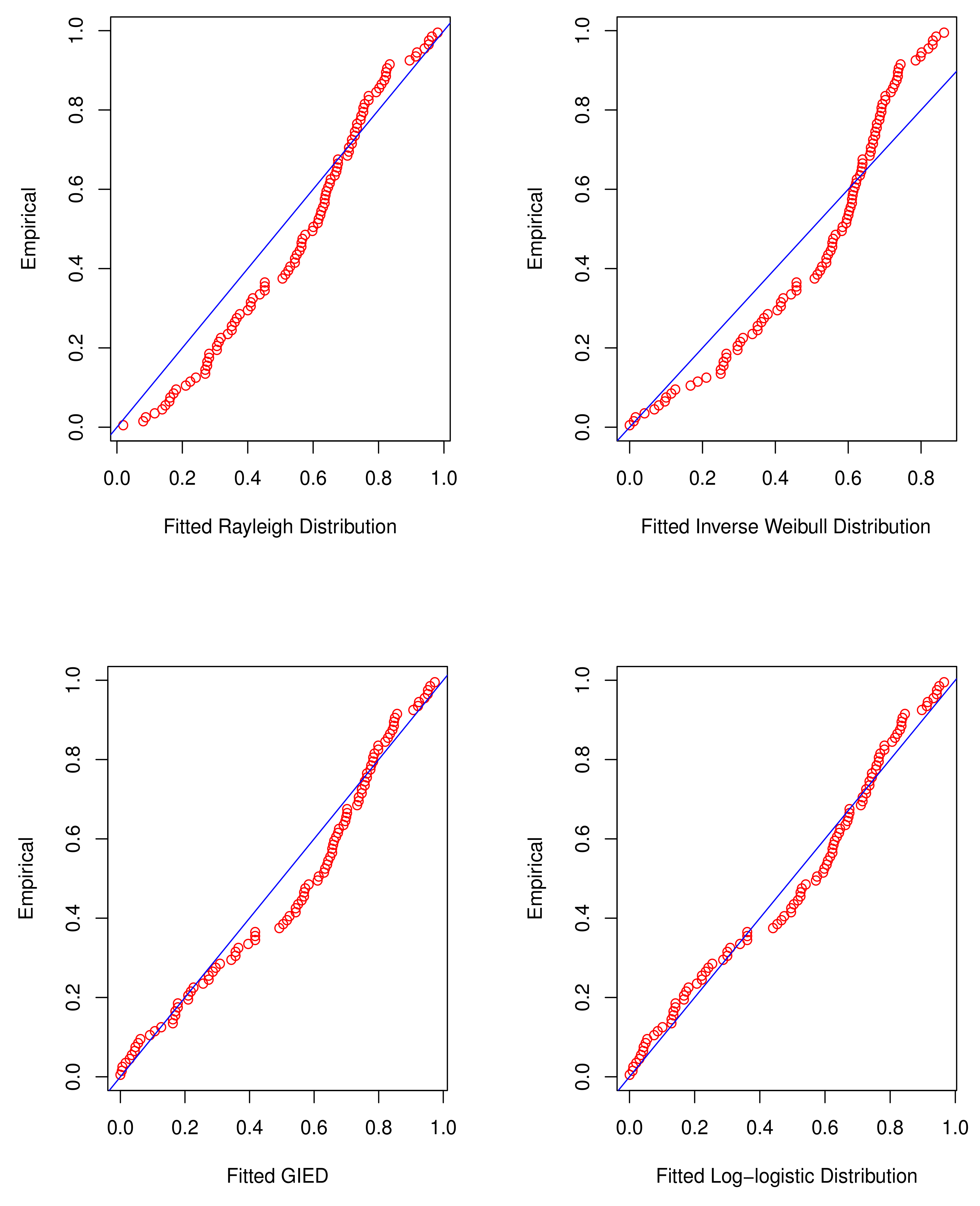
| Distribution | MLEs | -lnL | AIC | BIC | K-S | p-Value |
|---|---|---|---|---|---|---|
| Rayleigh | 149.0086 | 300.0172 | 302.6224 | 0.1402 | 0.039263 | |
| Inverse Weibull | 172.4966 | 348.9931 | 354.2035 | 0.1761 | 0.004038 | |
| GIED | 150.4161 | 304.8322 | 310.0426 | 0.1330 | 0.058198 | |
| Log-logistic | 145.3980 | 294.7960 | 300.0064 | 0.0860 | 0.449972 | |
| 0.39 | 0.81 | 0.85 | 0.98 | 1.08 | 1.12 | 1.17 | 1.18 | 1.25 | 1.36 | 1.41 | 1.47 | 1.57 | 1.57 | 1.59 | 1.59 |
| 1.61 | 1.69 | 1.69 | 1.71 | 1.73 | 1.80 | 1.84 | 1.84 | 1.89 | 1.92 | 2.00 | 2.03 | 2.05 | 2.17 | 2.35 | 2.41 |
| 2.48 | 2.50 | 2.53 | 2.55 | 2.59 | 2.74 | 2.82 | 2.88 | 2.95 | 2.97 | 2.97 | 3.19 | 3.19 | 3.27 | 3.28 | 3.31 |
| 3.60 | 3.75 |
| Censoring Scheme | |||
|---|---|---|---|
| 3.0026 ( 2.7037,3.3014) | 2.8616 (2.4917,3.2315) | 2.5402 (2.1406,2.9398) | |
| 5.1557 (3.6353,6.6761) | 3.9363 (2.7578,5.1148) | 3.3795 (2.31100,4.4480) | |
| 1.8021 | 1.2854 | 0.9945 | |
| 3.0241 | 2.9038 | 2.5987 | |
| 5.0412 | 3.8403 | 3.2878 | |
| 2.3527 | 1.5038 | 1.1405 | |
| 2.9774 (2.1088,3.1307) | 2.9453 (2.1960,3.1280) | 2.4499 (2.0829,2.6401) | |
| 4.6815 (3.6730,5.7100) | 3.6493 (3.1578,4.9303) | 3.7345 (3.2811,4.5882) | |
| 1.6024 | 1.1778 | 1.1097 |
| Censoring Scheme | Sample |
|---|---|
| 0.39, 1.80, 1.84, 1.84, 1.89, 1.92, 2.00, 2.03, 2.05, 2.17, 2.35, 2.41, 2.48, 2.50, 2.53, 2.55, 2.59, 2.74 | |
| 2.82, 2.88, 2.95, 2.97, 2.97, 3.19, 3.19, 3.27, 3.28, 3.31, 3.60, 3.75 | |
| 0.39, 1.47, 1.57, 1.57, 1.59, 1.59, 1.61, 1.69, 1.69, 1.71, 1.73, 1.80, 1.84, 1.84, 1.89, 1.92, 2.00, 2.03 | |
| 2.05, 2.17, 2.35, 2.41, 2.48, 2.50, 2.53, 2.55, 2.59, 2.74, 2.82, 2.88 | |
| 0.39, 0.81, 0.85, 0.98, 1.08, 1.12, 1.17, 1.18, 1.25, 1.36, 1.41, 1.47, 1.57, 1.57, 1.59, 1.59, 1.61, 1.69 | |
| 1.69, 1.71, 1.73, 1.80, 1.84, 1.84, 1.89, 1.92, 2.00, 2.03, 2.05, 2.17 |
| Censoring Scheme | Criterion | ||||
|---|---|---|---|---|---|
| det | trace | ||||
| 0.0130 | 0.6250 | ||||
| 0.0102 | 0.3972 | 0.0259 | 0.0428 | 0.0317 | |
| 0.0303 | 0.0611 | 0.0407 |
© 2020 by the authors. Licensee MDPI, Basel, Switzerland. This article is an open access article distributed under the terms and conditions of the Creative Commons Attribution (CC BY) license (http://creativecommons.org/licenses/by/4.0/).
Share and Cite
Xie, Y.; Gui, W. Statistical Inference of the Lifetime Performance Index with the Log-Logistic Distribution Based on Progressive First-Failure-Censored Data. Symmetry 2020, 12, 937. https://doi.org/10.3390/sym12060937
Xie Y, Gui W. Statistical Inference of the Lifetime Performance Index with the Log-Logistic Distribution Based on Progressive First-Failure-Censored Data. Symmetry. 2020; 12(6):937. https://doi.org/10.3390/sym12060937
Chicago/Turabian StyleXie, Ying, and Wenhao Gui. 2020. "Statistical Inference of the Lifetime Performance Index with the Log-Logistic Distribution Based on Progressive First-Failure-Censored Data" Symmetry 12, no. 6: 937. https://doi.org/10.3390/sym12060937
APA StyleXie, Y., & Gui, W. (2020). Statistical Inference of the Lifetime Performance Index with the Log-Logistic Distribution Based on Progressive First-Failure-Censored Data. Symmetry, 12(6), 937. https://doi.org/10.3390/sym12060937