1. Introduction
Multiple-criteria decision making (MCDM) is a branch of decision making theory where the aim of an individual is to select the most acceptable alternatives among the feasible ones under some criteria. This criteria dependence in decision can be found in real life on a regular basis. While handling some real life decision making problems, a decision maker often faces trouble due to the presence of several kinds of uncertainties in the data, which is very natural. An attempt was made for the first time by Zadeh [
1] by introducing a novel concept of fuzzy set theory. Immediately after that, several improvisations of fuzzy sets were made and implemented in the decision making process. For instance, rough sets by Pawlak [
2], intuitionistic fuzzy sets [
3], interval valued intuitionistic fuzzy sets [
4] by Atanassov, soft sets by Molodtsov [
5], etc. Unlike the classical logic, a fuzzy set associates a degree of membership value to every element of the universe of discourse, which can range from 0 to 1, whereas an intuitionistic fuzzy set associate a degree of membership
and a degree of non-membership
, where
. The margin of indeterminacy or hesitation
is defined as
. Smarandache in [
6,
7] proposed neutrosophic sets. In neutrosophic sets, the indeterminacy membership function walks along independently of the truth membership or of the falsity membership. Neutrosophic theory has been widely explored by researchers (see [
8,
9,
10,
11,
12,
13]) for application purpose in handling real life situations involving uncertainty. Although the hesitation margin of neutrosophic theory is independent of the truth or falsity membership, looks more general than intuitionistic fuzzy sets yet. Recently, in [
14] Atanassov et al. studied the relations between inconsistent intuitionistic fuzzy sets [
15], picture fuzzy sets [
16], neutrosophic sets [
7] and intuitionistic fuzzy sets [
3]; however, it remains in doubt that whether the indeterminacy associated to a particular element occurs due to the belongingness of the element or the non-belongingness. This has been pointed out by Chattejee et al. [
17] while introducing a more general structure of neutrosophic set viz. quadripartitioned single valued neutrosophic set (QSVNS). The idea of QSVNS is actually stretched from Smarandache’s four numerical-valued neutrosophic logic [
18] and Belnap’s four valued logic [
19], where the indeterminacy is divided into two parts, namely, “unknown” i.e., neither true nor false and “contradiction” i.e., both true and false. In the context of neutrosophic study however, the QSVNS looks quite logical. Also in their study, Chatterjee et al. [
17] analyzed a real life example for a better understanding of a QSVNS environment and showed that such situations occur very naturally. They have also solved a decision making problem pertaining to pattern recognition showing the application capability of QSVNS.
Bipolarity often reflects the tendency of the human mind in reasoning to make a decision on the basis of +ve and -ve information. Lee [
20,
21] introduced bipolar fuzzy set as an extension of fuzzy set. Bipolar fuzzy model with some hybrid structures were studied in [
22,
23,
24,
25] shows the flexibility of bipolar fuzzy sets for solving decision making problems. Bipolar fuzzy set and neutrosophic set have been put together for a more general framework viz. bipolar neutrosophic sets (BNS) by Deli et al. [
26]. Sahin et al. [
27,
28] introduced the Jaccard vector similarity measure, hybrid vector similarity measure, and dice similarity measure with applications to decision making problems. Jamil et al. [
29] applied bipolar neutrosophic Hamacher averaging operator in group decision making problems. Bipolar neutrosophic sets help in handling uncertain information in a reliable way. It is an extension of the bipolar fuzzy set and neutrosophic set, which can deal with real life problems involving positive and negative information. Looking at the work of Chatteree et al. [
17], unlike neutrosophic set, it is in doubt whether the negative indeterminacy associated to some elements of the universe of discourse is due to the occurrence of the counter-property or the non-occurrence of the counter-property.
To overcome the aforesaid situation we merged the bipolar neutrosophic set and QSVNS to introduce a more general structure, namely, quadripartitioned single valued bipolar neutrosophic sets (QSVBNS). The word “quadripartitioned” refers to four values i.e., in case of QSVBNS the negative indeterminacy of the BNS is divided into two parts alongside truth and falsity membership alike QSVNS.
First, we develop some set theoretic results on QSVBNS and then formulas for similarity measures were framed, and finally a real life problem was dealt with using the MCDM method in this setting. A comparison was made in application of a real life problem, where it is seen that the use of QSVBN system gives a better result compared to fuzzy sets and bipolar fuzzy sets. The paper is organized as follows:
Section 2 recalls some preliminaries results. In
Section 3, QSVBNS is introduced and some basic operations on QSVBNS are dealt with; an example of QSVBNS is also presented. Several similarity measures between QSVBNS are defined and their properties are studied in
Section 4. In
Section 5 we give an algorithm based on quadripartitioned bipolar weighted similarity measure to deal with the multi-criteria decision making problem in a QSVBN environment. Based on the given algorithm, a real life problem in decision making is solved in
Section 6. A detailed discussion about the obtained result is analyzed in
Section 7. Finally,
Section 8 concludes the paper.
3. Quadripartitioned Single Valued Bipolar Neutrosophic Sets
In this section, we introduce the concept of quadripartitioned single valued bipolar neutrosophic sets (QSVBNS).
Definition 6. A quadripartitioned single valued bipolar neutrosophic set (QSVBNS) A in X defined as an object of the form , where, and . The positive membership degrees denote respectively the truth-membership, a contradiction-membership, an ignorance membership, and falsity membership of corresponding to a QSVBNS A. The negative membership degrees denote respectively the truth-membership, a contradiction- membership, an ignorance membership, and falsity membership of to some explicit counter-property corresponding to a QSVBNS A.
With respect to and and +ve and -ve membership grade, there is a sense of symmetry in the structure of QSVBNS.
Example 1. Suppose an environment organization desires to know peoples opinion on the following statement:
“The fashion industry has helped economic growth but it also has a bad impact on the environment due to a large amount of carbon emissions”.
To help the cause, a group of four experts, say , has been asked to give their opinion. The statement can be divided into two parts as:
- (a)
The fashion industry has helped economic growth and to a counter property of that:
- (b)
The fashion industry has a bad impact on the environment due to a large amount of carbon emissions.
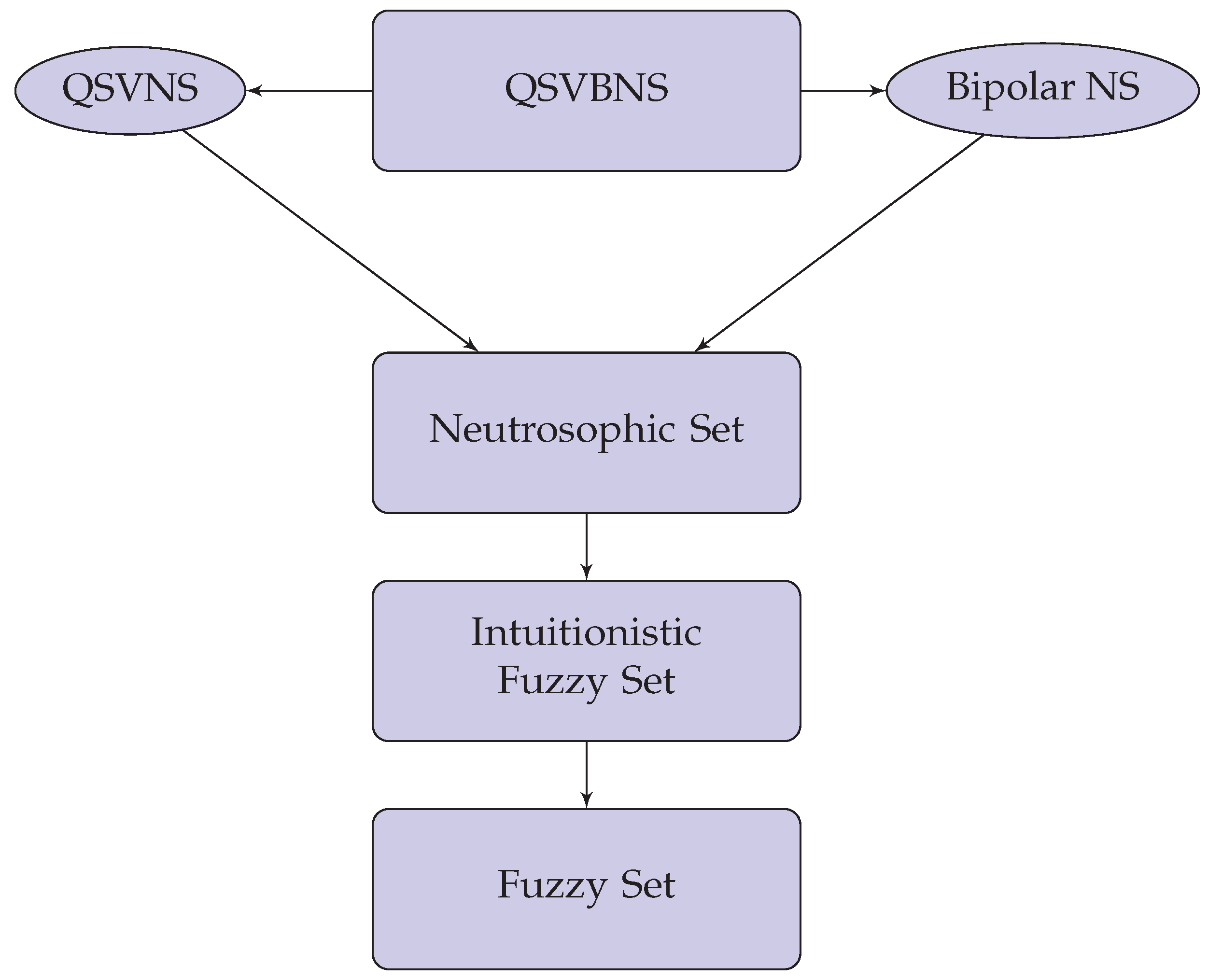
It may so happen that the opinion has the following outcomes: “a degree of agreement with statement and disagreement with statement ”, “a degree of agreement and disagreement with both the statements and ”, “a degree of neither agreement nor disagreement regarding both the statements”, and “a degree of disagreement with statement and agreement with statement ”. According to the views of the four experts, the outcome represented in terms of QSVBNS as follows:the above QSVBNS reflects that the expert agrees to the fact that the fashion industry has helped economic growth, whereas the expert believes that fashion industry might have helped economic growth but it also has affected the environment a bit. On the other side the expert is ignorant regarding the truth of both the statements and the expert opines that fashion industry does not have much impact on the world economy but he believes that it causes damage to the environment. Remark 1. The relationship between QSVBNS and other extensions of fuzzy sets are diagrammatically depicted in the following figure (Figure 1). Definition 7. A QSVBNS, A over a universe X is said to be an absolute QSVBNS, denoted by , if for each .
Definition 8. A QSVBNS, A over a universe X is said to be a null QSVBNS, denoted by Θ, if for each the membership values are respectively .
Alongside this, we expound some set theoretic operations on quadripartitioned single valued bipolar neutrosophic sets over a universe X and analyze some of their properties.
Definition 9. Let A and B be two QSVBNS over X. Then A is said to be included in B, denoted by , if for each and .
Definition 10. Two QSVBNSs A and B are said to be equal if for each and .
Definition 11. The complement of a QSVBNS A, denoted by , is defined as, , where, and .
Definition 12. The union of two QSVBNS A and B, denoted by is defined as, .
Definition 13. The intersection of two QSVBNS, A and B, denoted by is defined as, .
Example 2. For two QSVBNS A and B over X given by and
- (1)
.
- (2)
.
- (3)
.
Theorem 1. Under the aforesaid set-theoretic operation, the quadripartitioned single valued bipolar neutrosophic sets satisfy the following properties:
- (1)
Identity law:
- (2)
Commutative law:
- (3)
Associative law:
- (4)
Distributive law:
- (5)
De-Morgan’s law:
Proof. Proofs are plain-dealing. □
4. Similarity Measure of Quadripartitioned Bipolar Neutrosophic Sets
Here we provide the definition of similarity measure between two QSVBNS over a universe X.
Definition 14. Let QSVBNS(X) indicate the set of all QSVBNS over the universe X. Let be a function satisfying the following properties for all :
- (S1)
and iff ,
- (S2)
,
- (S3)
for any with , .
then S is said to be a similarity measure.
Based on the membership functions of two QSVBNS, we prescribe some functions which measures the differences between the membership values of two QSVBNS. Let QSVBNS. For each and for each and define the functions
QSVBNS(X) respectively,
,
,
,
,
,
.
Remark 2. The function defined by QSVBNS is shown to be a similarity measure in the following theorem.
Theorem 2. is a similarity measure between two quadripartitioned bipolar neutrosophic sets A and B over X.
Proof. Since and for all it follows that attains its maximum value 1 whenever one of the positive truth membership values corresponding to A and B is 1 and the other is 0 and one of the negative truth membership values corresponding to A and B is and the other is 0. Similarly for each attains its minimum value 0 whenever and . Thus for all , . Likewise it can be shown that .
Therefore for all
we have,
Again, and .
It is easy to prove that .
Finally let
. Then for all
, we have
Then, .
Therefore, ...........................
Considering a similar process, it can be shown that and .
Similarly . Therefore, . Hence the proof. □
Remark 3. Define , where p, a positive integer, is defined to be the order of the similarity.
Theorem 3. is a similarity measure between two quadripartitioned bipolar neutrosophic sets A and B over X.
Proof. is quite obvious.
Under any of the the following condition attains its maximum value 1,
- (1)
and at least one of or is 0 or and at least one of or is 0,
- (2)
and at least one of or is 0 or and at least one of or is 0,
- (3)
and or and ,
- (4)
and or and .
Also the minimum value of
is 0. Thus
for all
. Also
follows from similar arguments. Therefore,
To show the triangular inequality suppose . Then for all , we have, .
Then and follows from of Theorem 2. Next consider and . From above inequalities we have, .
Similarly, .
Then,
Similarly it can shown that
.
It is identical to show . Therefore, . This completes the proof. □
We define below the weighted similarity measure between two QSVBNS over a universe X.
Definition 15. The weighted similarity measure of two QSVBNS is defined as, , where, is the weight vector assigned to the element of the universe X, such that and .
It is effortless to find out that satisfies the conditions of similarity measure.
Remark 4. We define the following functions based on one particular membership function for two QSVBNSs A and B over the universe of discourse X, provided the denominators never vanish The following is a definition of generalized similarity measure between two QSVBNS whose value set is the set of all matrices over .
Definition 16. Let be a finite universe of discourse. For two QSVBNSs define a mapping QSVBNS QSVBNS byand a partial order relation “⪯” on as:Also define Remark 5. Then for QSVBNS
- (1)
,
- (2)
,
- (3)
for .
We give an outline of the proof as:
Let . Then for all . Consequently, , max, min, max .
Then we have, .
A similar process follows for . Hence .
Hence is a generalized similarity measure.
Definition 17. Let QSVBNSQSVBNS be a mapping satisfying the following conditions:
- (d1)
and iff ,
- (d2)
,
- (d3)
.
Then d is said to be a distance based measure between two QSVBNS A and B.
We now define the Hamming distance, normalized Hamming distance, Euclidean distance, and normalized Euclidean distance between two QSVBNSs QSVBNS,
- (1)
The Hamming distance:
• ,
- (2)
Normalized Hamming distance:
• ,
- (3)
The Euclidean distance:
• ,
- (4)
Normalized Euclidean distance:
• .
7. Discussion
In this section, a detailed analysis about the above introduced algorithm and the obtained result based on the algorithm is carried through. The weighted quadripartitioned similarity measure between the alternatives (
and the positive ideal quadripartitioned bipolar neutrosophic solution is shown in
Table 2 and the same with the negative ideal quadripartitioned bipolar neutrosophic solution is given in
Table 2. The main objective of the proposed algorithm i.e., the average ideal solution is obtained. The ranking results based on these similarity measures is highlighted in the final Table (
Table 3).
Deli et al. [
28] and Sahin et al. [
27], in their study on bipolar neutrosophic sets, obtained the ranking result without considering the negative ideal solution. From their algorithm, it can be seen that if the decision maker is asked to choose an alternative emphasizing more on the satisfaction degree of the given criteria than the satisfaction degree of the counter-property of the criteria, the similarity measure with the positive ideal solution can be used to get the most suitable alternatives. In the reverse case, the similarity measure with negative ideal solution will be more fruitful.
In the case of QSVBNS, our algorithm follows the same footstep as Deli et al. [
28]; however, the major difference is that we have used the average of the measure values of positive ideal solution and negative ideal solution. From the proposed algorithm, it seems that the ranking results to choose the best alternatives using a positive ideal solution and a negative ideal solution will give exactly the opposite ranking, but this is not the case, as can be seen in
Table 2. The similarity index
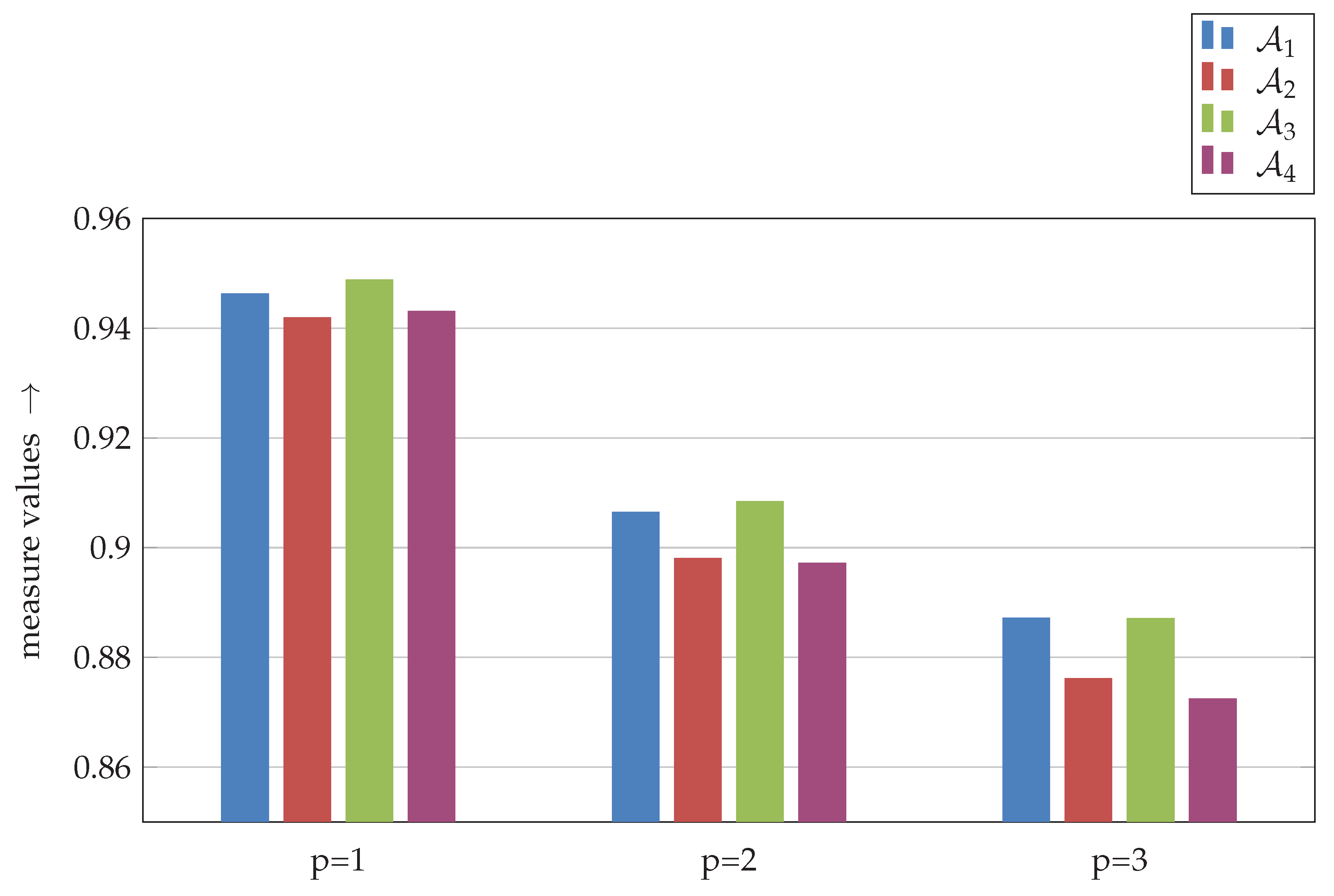
p in the weighted quadripartitioned similarity measure also has a big role to play. From the study, we have found that as the similarity index starts to take more higher values, the formula predicts more accurately, as the difference between the first two choices of the alternatives starts increasing for higher values of
p. From
Figure 2, it is observed that for
, the alternative values are quite close and
comes out as the best alternative with a very small margin from
. For
,
overtakes
as the best alternative and as
p stars increasing,
remains the best among the four alternatives and the margin of the second best choice
starts increasing. The differences between the alternative values is shown in
Figure 2 for
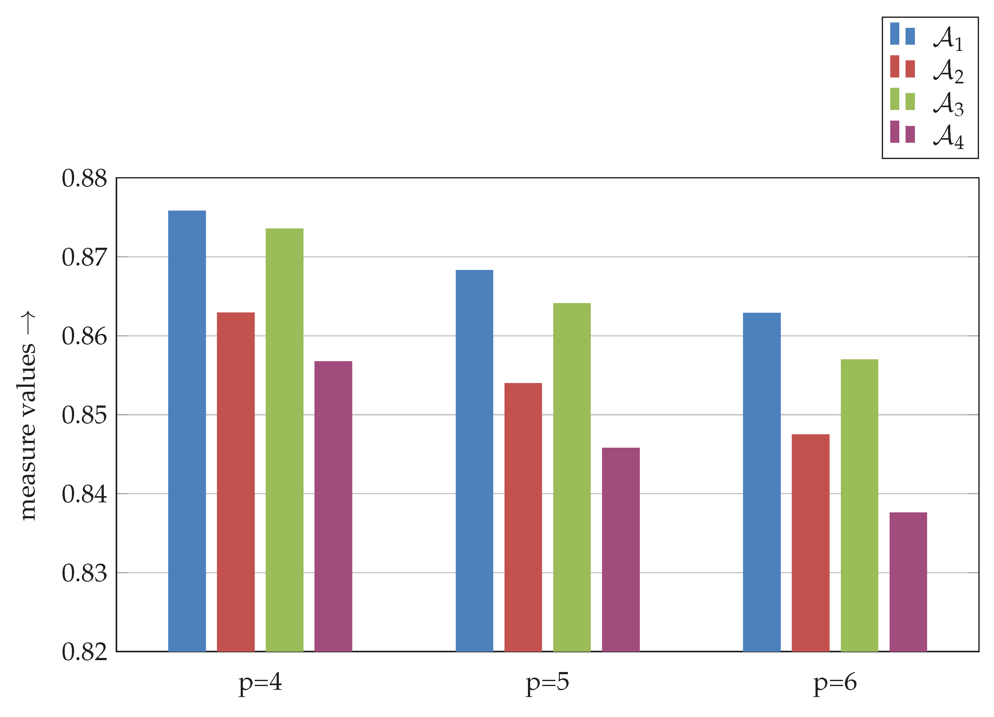
. In
Figure 3, it can be observed that for
enlarge by a bit more margin than
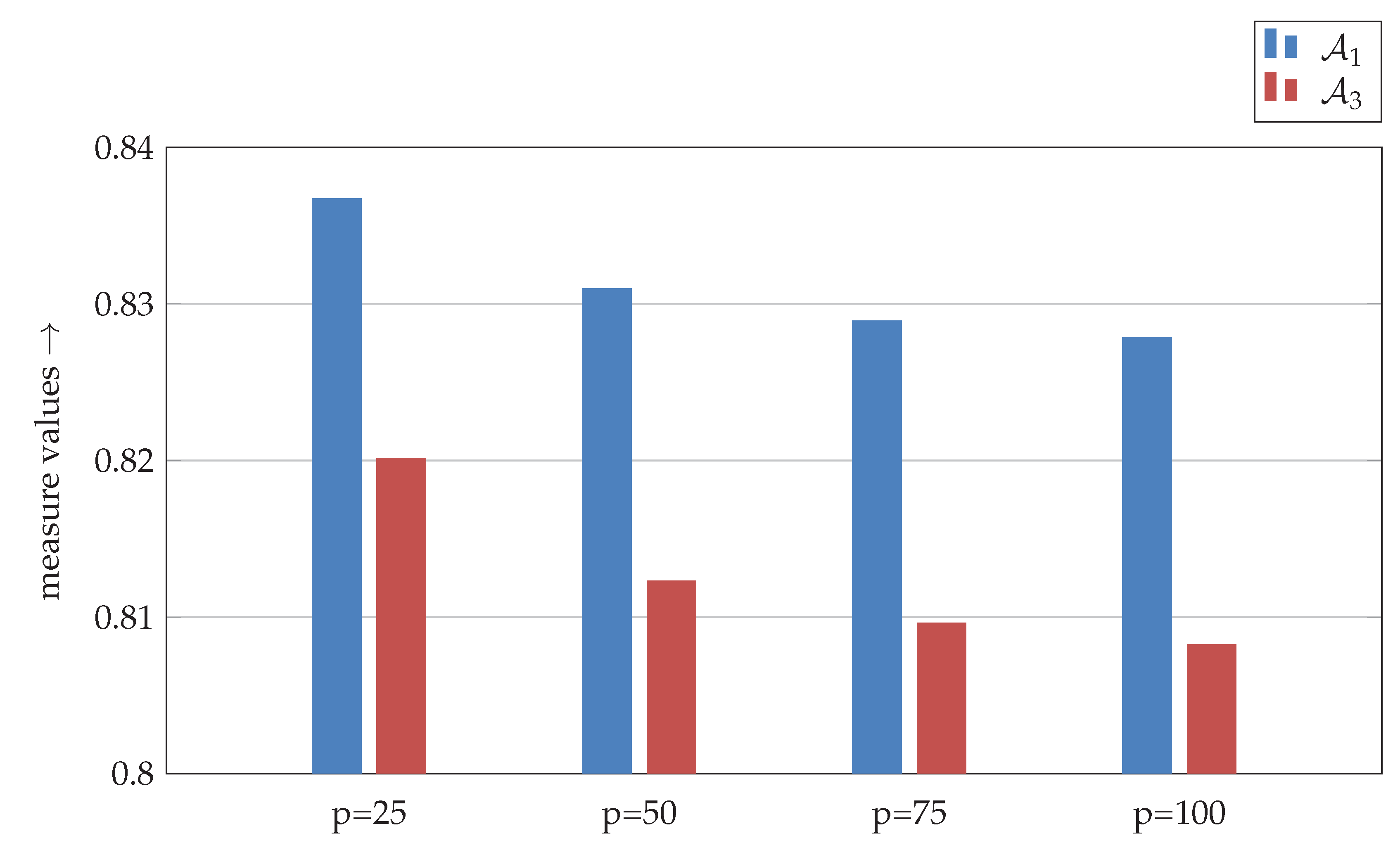
. In
Figure 4, the comparison between the best two alternatives
and
is shown. It can be seen that for a very large value of
p,
.
From the above analysis it is clear that is the most suitable alternative to the decision maker. The proposed method can get the better of the decision making problem with quadripartitioned bipolar neutrosophic information. Also, the higher similarity index produces a more accurate method by indicating clear differences between the alternatives. A comparison of the above discussed MCDM problem is made in a fuzzy system and a bipolar fuzzy system, where it is observed that in a fuzzy system, the same conclusion is reached at and in bipolar fuzzy system the result fluctuate between and . So, we think that the proposed method can serve immensely in decision making purpose.


