Article

CryptoDL: Predicting Dyslexia Biomarkers from Encrypted Neuroimaging Dataset Using Energy-Efficient Residue Number System and Deep Convolutional Neural Network

by
Opeyemi Lateef Usman
* and
Ravie Chandren Muniyandi
Research Centre for Cyber Security, Faculty of Information Science and Technology, University Kebangsaan Malaysia, UKM Bangi 43600, Selangor, Malaysia
*
Author to whom correspondence should be addressed.
Symmetry 2020, 12(5), 836; https://doi.org/10.3390/sym12050836
Submission received: 15 February 2020 / Revised: 25 March 2020 / Accepted: 26 March 2020 / Published: 20 May 2020

Abstract

:
The increasing availability of medical images generated via different imaging techniques necessitates the need for their remote analysis and diagnosis, especially when such datasets involve brain morphological biomarkers, an important biological symmetry concept. This development has made the privacy and confidentiality of patients’ medical records extremely important. In this study, an approach for a secure dyslexia biomarkers classification is proposed using a deep learning model and the concept of residue number system (RNS). A special moduli set of RNS was used to develop a pixel-bitstream encoder that encrypts the 7-bit binary value of each pixel present in the training and testing brain magnetic resonance imaging (MRI) dataset (neuroimaging dataset) prior to classification using cascaded deep convolutional neural network (CNN). Theoretical analysis of our encoder design shows that the proposed pixel-bitstream encoder is a combinational circuit that requires fewer fast adders, with area complexity of 4n AFA and time delay of (3n + 3) DFA for n ≥ 3. FPGA implementation of the proposed encoder shows 23.5% critical path delay improvement and saves up to 42.4% power. Our proposed cascaded deep CNN also shows promising classification outcomes, with the highest performance accuracy of 73.2% on the encrypted data. Specifically, this study has attempted to explore the potencies of CNN to discriminate cases of dyslexia from control subjects using encrypted dyslexia biomarkers neuroimaging dataset. This kind of research becomes expedient owing to the educational and medical importance of dyslexia.

1. Introduction

An important source of diagnostic information for clinicians and medical experts is the analysis and interpretations of medical images. Medical images have been taken through various medical imaging techniques, such as X-ray machine, mammography, ultrasound scanner, magnetic resonance imaging (MRI), computed tomography (CT), positron emission tomography (PET), and so on [1]. Such images were used in different ways to detect and treat diseases early by exposing their structural anatomical variances to normal biological/pathological processes, better known as biomarkers [2,3]. In the context of brain tissue morphology, function, and cortical geometry properties, such anatomical structures are referred to as neuro-biomarkers. MRI tools allow medical doctors and researchers to visualize and analyze alterations in the anatomy of the brain [4] and are available in three different types: functional MRI (fMRI), structural MRI (sMRI), and diffusion tensor imaging (DTI) [5,6]. These tools generate the best brain soft-tissue resolutions and have been used to capture and analyze different brain regions [5,6,7], using information provided by them to diagnose various critical brain diseases and learning disabilities such as mild cognitive impairment, Alzheimer’s, dementia, schizophrenia, Williams syndrome, Landau–Kleffner syndrome, autism, attention deficit hyperactivity disorder (ADHD), and dyslexia, among others [7,8].
Identifying and classifying learning difficulties has economic implications on a nation. Dyslexia, as a learning disability, affects the child’s academic life and self-esteem into adulthood [9], hence its early diagnosis through accurate classification of biomarkers contained in the brain MRI dataset (neuroimaging dataset) is a crucial step towards the provision of appropriate technological interventions [10], and to consequently enable children to maximize their educational potentials.
Development in machine learning has made classification of dyslexia biomarkers easy, with promising accuracy. In an attempt to predict biomarkers of dyslexia, previous studies have used machine learning techniques in the form of artificial neural networks (ANNs) with fewer hidden layers and support vector machine (SVM) [11,12] to diagnose the conditions of dyslexia, but studies are uncommon on the application of deep learning models for this type of scenario [13], particularly from the brain MRI dataset. Deep learning techniques [14] are advanced artificial neural networks. Deep learning models such as convolutional neural network (CNN), auto-encoders, stacked auto-encoders, deep belief network (DBN), and a restricted Boltzmann machine (RBM) have demonstrated state-of-the-art performance in computer vision and image analysis efficiency [15,16]. An illustrative example is the 2012 ImageNet Competition (ILSVRC) [17], where prediction accuracy was improved by more than 15% compared with the best model of the previous year. The general advantages of deep learning over conventional machine learning are that deep models automatically learn abstract hierarchical feature representations directly from data, thereby removing the feature extraction engineering step inherent in the machine learning model [1,2,3,4].
With the increasing availability of the medical imaging dataset, cloud deployment of deep leaning techniques has become expedient and has attracted greater attention recently; for example, Microsoft Azure Machine Learning Studio and Google Cloud Machine Learning Engine (Google Prediction API), GraphLab, and Ersatz Labs [18,19,20]. In this situation, the privacy of patients’ information is extremely important and needs urgent attention [21], particularly when a learning disability biomarkers dataset such as dyslexia is involved. To address the privacy issue in medical image, Al-Haj et al. [22] developed a crypto-based algorithm that ensures a safe exchange of medical images along the transmission channel. These algorithms are based on cryptographic function and internally generated primary keys. In a similar manner, a chaotic map cryptographic algorithm has been proposed by Gatta and Al-Latif [23] based on pixel confusion and diffusion processes. Meanwhile, Pengtao et al. [20], Dowlin et al. [24], and Chao et al. [25] have independently suggested the use of mathematically efficient homomorphic cryptography to ensure privacy of sensitive images for a remote classification, a concept generally referred to as CryptoNet and CryptoDL, respectively. In the methods of [22] and [23], the confusion process changes pixels’ locations in the plain image, while the diffusion process transforms an individual pixel’s value in order to eliminate the correlation between pixels of plain image and chaotic image. Following the confusion paradigm proposed in [23], Koppu and Viswanatham [26] proposed an image encryption approach based on a miscellaneous dataset of University of Southern California-Signal and Image Processing Institute (USC-SIPI) using hybrid chaotic magic transform (HCMT), liner congruential generator (LCG), and Lanczo’s algorithms. In the process, the LCG random value was used by the HCMT algorithm to shuffle the position of the pixel in the plain image to create a chaotic cipher-image, while the Lanczo’s algorithm was used to perform normalization on large eigenvalues and eigenvectors, respectively. These proposed algorithms only dealt with the security of medical images during transmission, and no consideration is given to the need for remote classification of such encrypted medical images. Apart from other security flaws of these algorithms [27], the confusion process of algorithms in [23] and [26], respectively, tends to adversely affect the classification outcome when such an encrypted image is subjected to deep model classification owing to the distortion of the region of interest (ROI) that is important to the classification results.
Residue number system (RNS) is a modular arithmetic-based, non-weighted number system [28], unlike conventional binary and decimal number systems. Its carry-free computation and parallelism properties have been exploited in various digital signal processing (DSP) applications such as filtering, Fourier transforms (discrete and fast), and cryptography [29]. It has widely been used either singly [30] or in combination [31] with other methods to encrypt both text-based and digital image datasets [32,33,34]. Using the RNS concept along with deep learning on medical images dataset presents novel research in the machine learning era, as well as an important breakthrough in patients’ information privacy preservation in medicine, thereby corroborating the concept of “CryptoDL” described in the previous studies. In this study, a medical image classification and encryption method is proposed. RNS with a special moduli set was used to design a bitstream encoder that encrypts MRI sourced brain image datasets (neuroimaging datasets) before classifying them using cascaded deep CNN. The objective of this secure classification is to obtain, from the knowledge embedded, the possibility of predicting the biomarkers of dyslexia from the encrypted neuroimaging dataset. To prevent overfitting issues, however, our method attempted to augment encrypted data through the creation of multiple image patches in order to increase the quality of the proposed deep learning model. This approach is rarely implemented in image encryption [35]. Advantageously, augmentation increases the number of data points used to train the deep model to prevent overfitting [36].
The entire paper is organized into six sections. Section 2 and Section 3 provide an overview of the deep convolutional neural network (CNN) and RNS-based encryption method for brain image datasets, respectively. The proposed research methodology is presented in Section 4, with emphasis on the design of a pixel-bitstream RNS encoder and deep CNN architecture, while Section 5 presents the experimental results followed by a detail discussion of the findings. Concluding remarks and future direction are provided in the sixth and final section.

2. An Overview of Deep CNN for Image Dataset Classification

Deep CNNs are special types of artificial neural networks (ANNs) that learn from the spatial information contained in digital images, hierarchical representations. It was originally designed to process multi-dimensional (2D and 3D) arrays of high-resolution input datasets such as images and videos using very few connections between the layers [1,2,3,4]. Inspired by a cat’s visual cortex, its origin is from the Neocognitron proposed by Fukushima in 1980 [37,38], while LeCun et al. [39] gave the first architecture in 1998 (LeNet-5). From 2012 till now, CNN has witnessed several major architectural innovations [40], among which the following are popular: AlexNet 2012, VGG 2014, GoogLeNet 2015, ResNet 2016, ResNexT 2017, and Channel Boosted CNN 2018 [41], to mention but a few. CNNs are able to form extremely well-organized representations of input images useful for image-oriented tasks, for example, classification. A CNN possesses several layers of convolutions and activations, often intertwined by pooling (or subsampling) layers and trained using backpropagation and gradient descent algorithms, similar to that of the popular feed-forward neural network (FFNN) [42,43]. Additionally, at the end, CNN usually has fully connected layers that compute the final output [44]. The layers of CNN are briefly described below:
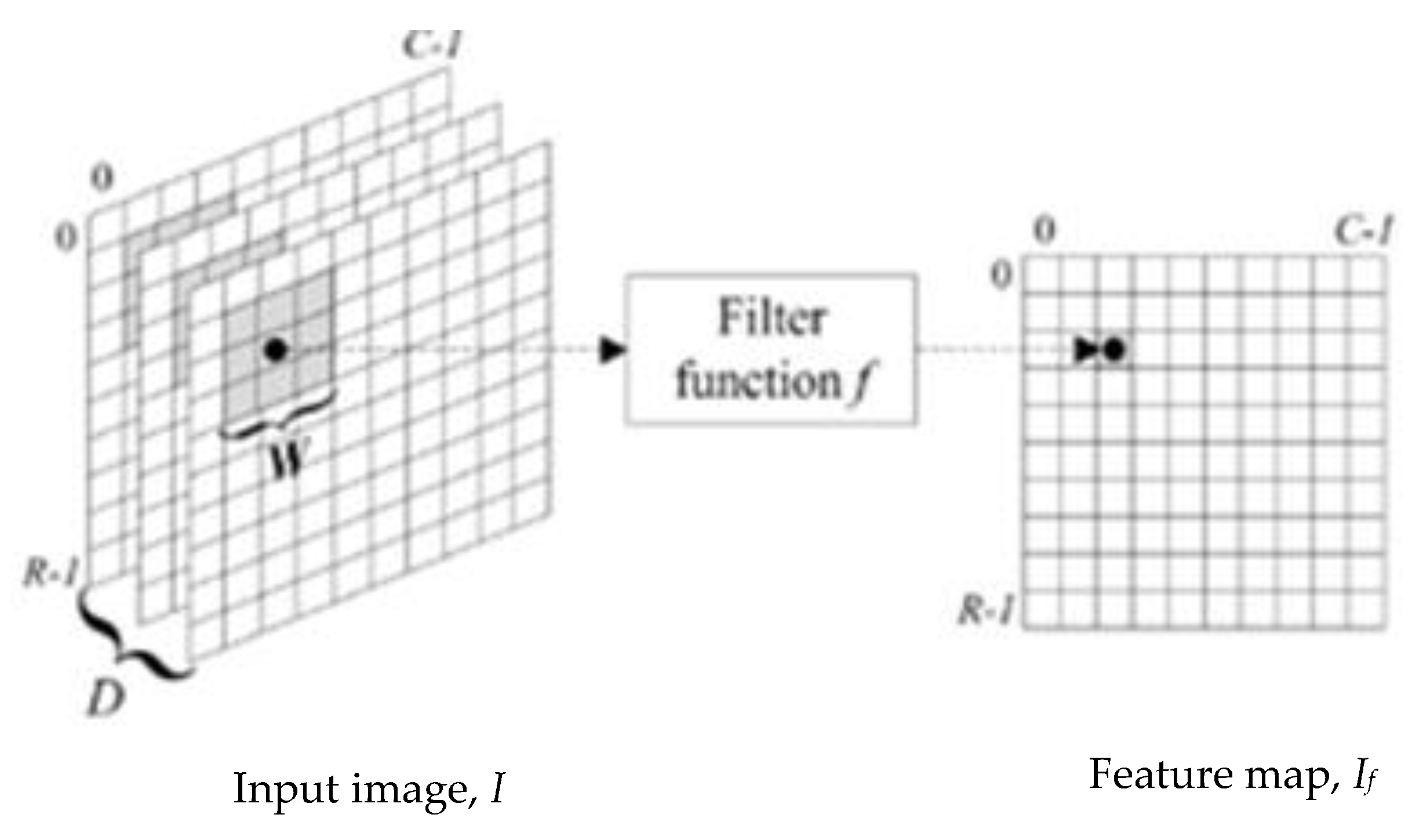
  • Convolutional Layer: A convolutional layer is a series of small parameterized filters that operate on the input data domain. In this study, inputs are raw brain images and encrypted brain images data. The aim of the convolutional layers is to learn abstract features from the data [45]. Every filter is an n × n matrix called a stride. In this case, we have n = 3. We convolve the pixels in the input image and evaluate the dot product, called feature maps, of the filter values and related values in the pixel neighbour. For example, the stride is a pair of numbers (3,3), in which, in each step, we slide a three-unit filter to the left or down. In summary, given a brain MRI image I (Figure 1), consisting of R rows, C columns, and D layers, a 2D function I (x, y, z) where 0 ≤ x < R, 0 ≤ y < C, and 0 ≤ z < D are spatial coordinates, amplitude I is called the intensity at any point on the 2D set with coordinates (x, y, z) [46]. The process of extracting feature maps is defined in Equation (1):
    I f ( x , y , z ) = k = 0 D 1 i = 0 n 1 j = 0 n 1 I ( x + i ,   y + j ,   z + k ) W i , j , k
    where If is the convolved image, and Wi,j,k are coefficients of kernels or strides for convolving 2D arrays.
  • Activation Layer: The feature maps from convolutional layers are inputted through a nonlinear activation function to produce another stride called feature maps [4]. After each convolutional layer, we used a nonlinear activation function. Each activation function performs some fixed mathematical operations on a single number, which it accepts as input. In practice, there are several activation functions from which one could choose. These include ReLU (ReLU (z) = max (0, z)), Sigmoid, Tanh functions, and several other ReLU variants such as leaky ReLU and parameter ReLU [4,45]. ReLU is an acronym for rectified linear unit.
  • Pooling Layer: A pooling layer, also known as sub-sampling layer, is next after an activation layer. The pooling layer takes small grid regions as input and performs operations on them to produce a single number for each region. Different kinds of pooling layers have been implemented in previous studies, with max-pooling and average pooling being the two most common. The pooling layers give CNN some translational invariance because a slight shift of the input image may result in a slight change in activation maps. In max-pooling (Figure 2), the value of the largest pixel among all the pixels is considered in the receptive field of the filter, while the average of all the pixel values is considered in average pooling.
  • Fully Connected Layer: The fully connected layer has the same structure as classical feed-forward network hidden layers. This layer is named because each neuron in this layer is linked in the previous layer to all neurons, where each connection represents a value called weight. Every neuron’s output is the dot product of two vectors, that is, neuron output in the preceding layers and the corresponding weight for each neuron.
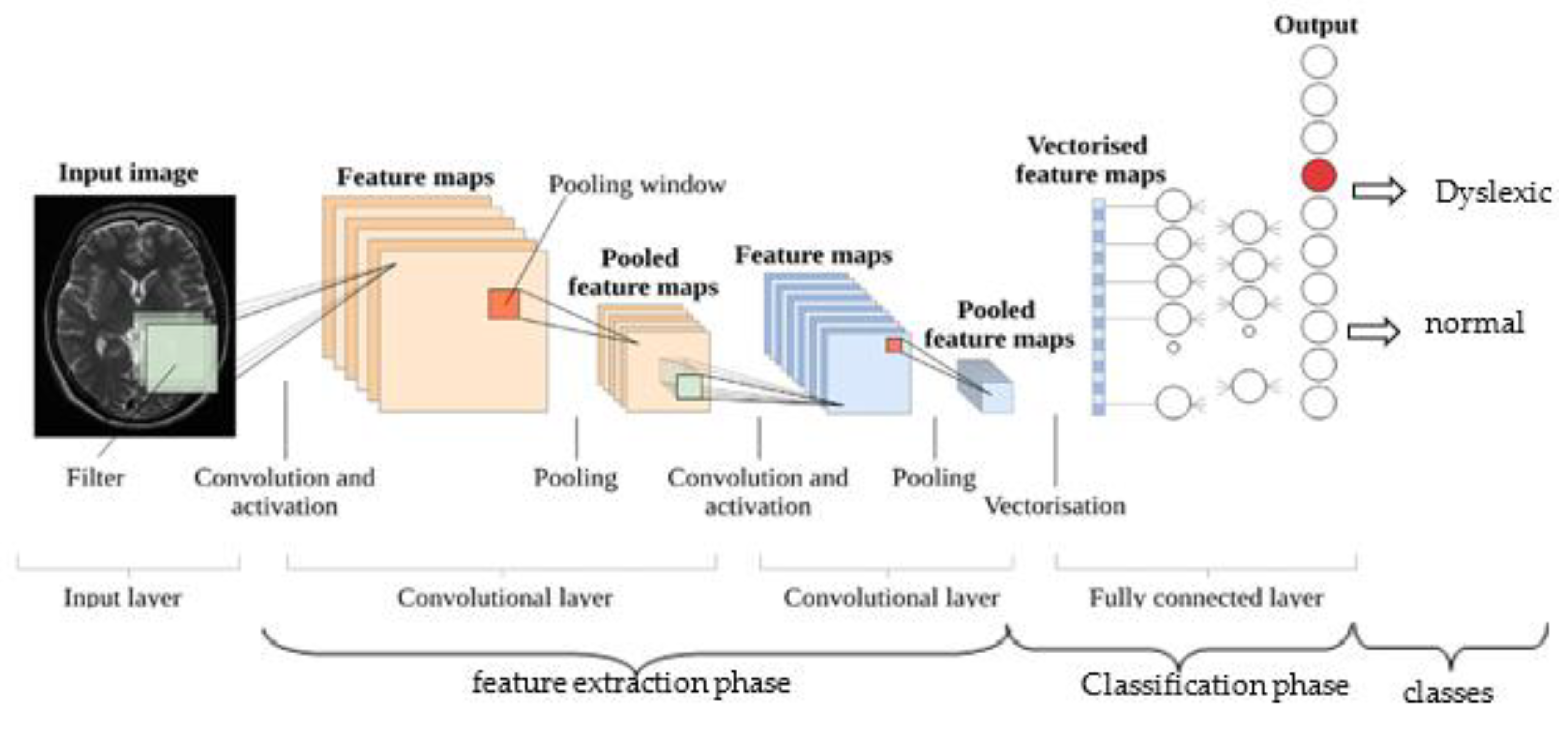
  • Dropout Layer: This layer is also called dropout regularization. A model sometimes gets skewed to the training dataset on many occasions, and when the testing dataset is added, it generates high errors. In this situation, a problem of overfitting has occurred. To avoid overfitting during the training process, we used a dropout layer. In this layer, by setting them to zero in each iteration, we dropout a set of connections at random in the fully connected layers. This value drop prevents overfitting from occurring, so that the final model will not be fully fit to the training dataset. Batch normalization is also used to resolve internal covariance shift issues within the feature maps by smoothing the gradient flow, thus helping to improve network generalization. Figure 3 shows the building blocks of the simplified deep CNN classifier for brain images.

3. Background of Residue Number System and Image Encryption

In modular arithmetic, a residue number system (RNS) represents a large integer using a collection of smaller integer called residues, so that computation can be more effectively performed [30]. Formally, RNS is expressed as the n-tuple of relatively prime moduli in pairwise form [47]. If S denotes the set of modules, then S = {m1, m2, …, mn} in such a way that GCD (mi, mj) = 1 is the greatest common divisor (GCD) provided ij. The dynamic range M of this RNS system is defined in Equation (2):
M = m 1 × m 2 × × m n = i = 1 n m i
Every integer XZM in the RNS can be expressed as X ( x 1 ,   x 2 ,   ,   x n ) using Equation (3):
r = | X | m i = X   m o d   m i
where ri = x1, …, xn represents residue; X is a large integer; mi is a module; and M represents the system dynamic range, which must be sufficiently large enough. ZM ranges from [0, M), called the legitimate range of X.
Residue number system (RNS) is able to support parallel, carry-free addition, and borrow-free subtraction and multiplication of a single step without partial product. These features make RNS useful in digital signal processing (DSP) applications including digital filtering, convolution, fast Fourier transform, discrete Fourier transform, image processing, and cryptography, among others [48]. However, ordered significance among the residue digits is less important, meaning that removal of some residue digits has no effect, except dynamic range reduction [33].
In image security, cryptography often conceals information, referred to as a plain image, and involves three important algorithms: keys generation, encryption, and decryption. Image encryption algorithms distort the original arrangement of pixels in an image, scramble them, and make them appear disorganized. RNS has been used to improve the performance of other traditional cryptographic algorithms such as Rivest Shamir and Adleman (RSA) [49], and data encryption standard (DES) [30]. Like all other digital images, the brain image is an array of pixels, sometimes called voxel. Each pixel corresponds to any numerical value between 0 and 225, where 0 represents black colour and 225 represents white colour. The value of a pixel at any point in a 7-bit grayscale image corresponds to the intensity of the light photons at that point.
In this study, a special moduli set of RNS was used to design pixel-bitstream encoder for the brain MRI dataset (neuroimaging dataset) before subjecting them to deep CNN classification (CryptoDL). The aim of our secure classification is the possibility of predicting dyslexia biomarkers from the encrypted neuroimaging dataset. Our proposed methodology is detailed in the subsequent section. However, the RNS cryptosystem requires the design of a binary-to-residue (BR) converter (encoder) circuit, which encodes each pixel bitstream during the encryption process, and a residue-to-binary (RB) converter circuit (decoder) to decrypt the encrypted bitstream to its equivalent pixel value during the decryption process. The latter can be implemented using variants of Chinese remainder theorem (CRT) [50], as well as mixed-radix conversion (MRC) algorithms [48,51].

4. Materials and Methods

4.1. Participants

The study sample neuroimaging dataset for our experiment consisted of 45 T1-weighted (T1w) images of school-aged adult population obtained from Kaggle Database. The sample comprised 19 dyslexics (mean age = 18.7 years; SD = 2.5576) and 26 control subjects (mean age = 19.0 years; SD = 2.5870) between the age range of 15–23 years. The overall participants’ mean age and standard deviation (SD) were 18.9 years and 2.5784 years, respectively. We can safely deduce from their age distribution information that the participants are mainly students, either in secondary schools or higher institutions of learning, comprising colleges of education, polytechnics, and universities, with a strong belief that a participant must have had at least ten years of formal education and an intelligence quotient (IQ) greater than 85 on a curriculum-based Wechsler Adult Intelligence Scale (WAIS). However, there is no information about their gender distribution. Meanwhile, our experimental model was tested on an unprocessed brain MRI dataset randomly selected from non-cancerous collections of data reserved for tumor segmentation challenge on Kaggle website. Expert analysis and interpretations used volumetric properties of grey matter, white matter, and cerebrospinal fluid tissues to classify the sample in the dataset into dyslexics and controls. Also, no participant was reported to have been diagnosed with hearing impairment; eyesight problems; or other critical neurological problems, for example, ADHD and Alzheimer’s disease.

4.2. Brain Images Acquisition and Pre-Processing

For the 19 dyslexic class, whole-brain scans were conducted using a 3T Siemens Tim Trio MRI scanner with a 32-channel head coil using the following acquisition parameters: acquisition matrix: 256 × 256 × 176; TR = 2300 ms; TE = 2.52 ms; flip angle = 9 deg; Field of View (FOV) = 256 mm; voxel size: 1 × 1 × 1 mm. Whole-brain scans were acquired with the use of 1.5 T Siemens Avento scanner with a 32-channel head coil for 26 control subjects. The following parameters were used: acquisition matrix: 256 × 256 × 170; TR = 1900; TE = 3.92 ms; flip angle = 15 deg; FOV = 256 mm; voxel size: 1 × 1 × 1 mm. The image dataset acquired was normalized and pre-processed in order to maintain uniform intensity by eliminating inherent heterogeneity caused by different scanner acquisition protocols [52]. From the normalized dataset, cognitive features relating to white matter, grey matter, and cerebrospinal tissues’ volumetric biomarkers were retrieved. These tissues are, therefore, the region of interest (ROI) necessary for deep learning classification. At the initial stage, all T1w neuro-images collected were transformed to FreeSurfer format [53], and normalized for intensity using a method of normalization of intensity based on histograms [54]. The skulls were subsequently removed using a skull-stripping algorithm [12,55], and the FSL FNIRT software tool [56] was used to perform non-rigid registration in the MNI152 brain template (MNI152 standard coordinate). To minimize noise, the registered images were modulated into Jacobian wrap field and smoothened using Gaussian isotropic kernel (Gaussian filter) with a kernel size of 4 mm [57].
After segmentation and registration, each image was split into a set of 50 small randomly overlapping patches of 16 × 16 pixels using some MATLAB codes. There were a total of 576,000 patches, comprising 243,200 patches for the dyslexia biomarker dataset and 332,800 patches for the control subject dataset. A small patch is generally more homogeneous than the entire image and can be more precisely classified [58]. Several patch-based image filtering algorithms exist, for example, Gaussian filter, and have been reported in the literature [59]. We explored binary digit 1 and 0 to label the patches, where 1 represents dyslexic and 0 represents normal. Each patch was resized to a height of 64 pixels to generated 64 × 64 pixel patches, which were used for deep CNN classification before and after encryption, respectively.

4.3. Proposed Conceptual Framework for Secure Brain Image Classification

The proposed conceptual framework for a secure classification of brain images consists of two parts, as shown in Figure 4: the image encryption part (Crypto) and deep CNN classification part (DL), respectively. As established in the introductory remarks, the encryption part was designed using a special moduli set of residue number system (RNS). The proposed RNS encryption is a pixel-based encryption algorithm in a similar manner as Sirichotedumrong et al. [35]. This algorithm allows a small number of parameters to train deep models to maintain the resolution value of an encrypted brain image, and is further discussed in Section 4.4.

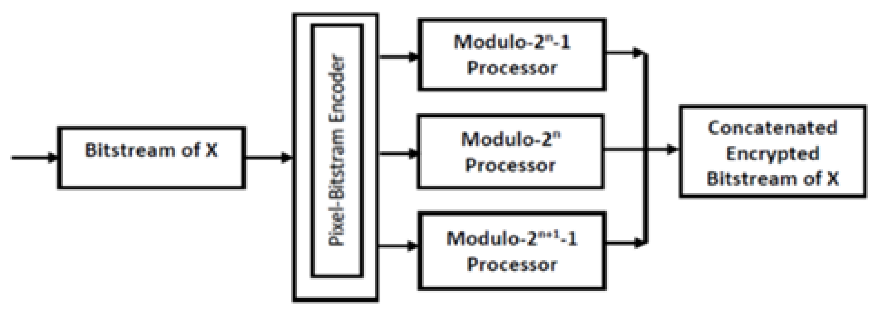
4.4. Design of RNS Pixel-Bitstream Encoder for Image Encryption

For the RNS encryption process, the moduli set {2n − 1, 2n, 2n+1 − 1} is suggested to establish bitstream shares for each pixel present in the patched brain image dataset, where m1 = 2n − 1, m2 = 2n, and m3 = 2n+1 − 1 represent the channel order of the modules with a value of n ≥ 3. These shares were concatenated to generate a cipher-image. In this scenario, the order of the moduli represents the public key (pk), while the value of n represents the secret key (sk), which must be kept as confidential as possible. In this scheme, a maximum cryptographic key length (λ = 4048 bits) was used for each modulo-channel to prevent adversarial forces such as brute-force, statistical, chosen plaintext, and chosen ciphertext attacks, because lower bit-length keys no longer provide enough strong security requirements. Designing a pixel bitstream encoder requires three parallel RNS modulo-processors, as illustrated in Figure 5. With the help of fast adders, each processor performs modular arithmetic operation regarding the arbitrary value of each corresponding mi modulus with the aid of carry save adders (CSA) and carry propagate adders (CPA), respectively.
Considering the above moduli set, to encode a pixel-bitstream X, we shall compute residues ri of each modulo-processor using Equation (3). This RNS system’s dynamic range M [60] is determined using Equation (2) as follows:
M = i = 1 3 m = ( 2 n 1 ) ( 2 n ) ( 2 n + 1 1 ) M = 2 3 n + 1 2 2 n + 2 n
The value of M indicates that pixel X is a (3n + 1)-bit integer. The expanded form of binary X is defined in Equation (5) as follows:
X = x 3 n x 3 n 1 x 3 n 2 x 1 x 0
where xi is either 0 or 1. Therefore, ri’s can be computed based on the following assumptions:
  • r2 is the n least significant bit (LBS) of integer X and is computed directly from modulo −2n processor.
  • For r1 and r3, X is partitioned into two n-bit blocks, Z1 and Z2, and one (n + 1)-bit block Z3, where
    Z 1 = j = 2 n 3 n x j 2 j 2 n + 1 Z 2 = j = n 2 n 1 x j 2 j n Z 3 = j = 0 n 1 x j 2 j }
This implies that
X = Z 1 + 2 n Z 2 + 2 2 n Z 3
As established in assumption (i), the most straightforward residue to be obtained is r2 in relation to modulo −2n, that is, r2 = Z1. The only requirement here is the determination of the values |2i|m and then the summation of the results with a reduction relative to modulus [61,62]. Two cases are to be considered here:

4.4.1. Case 1: Modulo −2n − 1

Encoding modulo −2n − 1 processor yields residue r1 as follows:
r 1 = | X | 2 n 1 = | Z 1 + 2 n Z 2 + 2 2 n Z 3 | 2 n 1 = | | Z 1 | 2 n 1 + | Z 2 2 n | 2 n 1 + | Z 3 2 2 n | 2 n 1 | 2 n 1 = | Z 1 + Z 2 + Z 3 | 2 n 1

4.4.2. Case 2: Modulo −2n+1 − 1

Similarly, encoding modulo −2n+1 − 1 processor yields residue r3 as follows:
r 3 = | X | 2 n + 1 1 = | Z 1 + 2 n Z 2 + 2 2 n Z 3 | 2 n + 1 1 = | | Z 1 | 2 n + 1 1 + | Z 2 2 n | 2 n + 1 1 + | Z 3 2 2 n | 2 n + 1 1 | 2 n + 1 1 = | Z 1 + 2 n Z 2 + 2 n 1 Z 3 | 2 n + 1 1
Example: Given the moduli set {2n − 1, 2n, 2n+1 − 1} where n = 3 and a pixel value X = 123 (i.e., 1111011 in binary). Then, the encoding process is as follows:
X = 123, which is equivalent to binary 1111011 (7-bit). From the design of our pixel-bitstream encoder, it was established that X = (3n + 1)-bit integer. As our secret key n = 3, we partition X into 3-bit blocks and 1-bit blocks starting from least significant bit (LSB).
Thus, Z1 = 011, Z2 = 111, and Z3 = 1.
Therefore, r2 = Z1 = 3 (011). Using Equations (8) and (9),
r 1 = | Z 1 + Z 2 + Z 3 | 2 n 1 = | 123 | 2 3 1 = | 3 + 7 + 1 | 7 = 4   ( 100 )
r 3 = | Z 1 + 2 n Z 2 + 2 n 1 Z 3 | 2 n + 1 1 = | 123 | 2 4 1 = | 3 + 2 3 ( 7 ) + 2 2 ( 1 ) | 15 = | 3 + 56 + 4 | 15 = | 63 | 15 = 3 ( 011 )
This implies that encoded pixel X contains 11100011 bits.
The hardware design of the encoder is realized using four fast adders: two carry save adders (CSAs) and two carry propagate adders (CPAs). CSAs perform 3-bit additions, while CPAs perform 2-bit additions, as shown Figure 6.
A CSA takes as input three operands, as shown in Figure 6: Z1, Z2, and Z3, and produces two outputs: a partial-sum (PS) and a partial-carry (PC), which must be fed into a CPA so that the carriages are propagated to produce an encoded result [61]. The architectural complexity area (A) and time delay (D) imposed on ri’s residues are calculated as follows from the above pixel-bitstream encoder:
A = [ C S A 1 + C S A 2 + C P A 1 + C P A 2 ] A F A = [ ( n 1 ) + ( n + 1 ) + ( n 1 ) + ( n + 1 ) ] A F A = 4 n A F A
D = [ C S A 2 + 2 C P A 2 ] D F A = [ ( n + 1 ) + 2 ( n + 1 ) ] D F A = ( 3 n + 3 ) D F A

4.5. Deep CNN Architecture, Training, and Classification

The simple architecture (Figure 3), which corresponds to a linear stack of several convolutional layers, accompanied by ReLU activation, brightness normalization, and overlapping layers of pooling, remains the commonly used deep CNN configuration in computer vision. However, various improvements were made to the above-mentioned architecture in terms of parameter optimization, regularization, and structural reformation to mention but a few, through the redesign of its processing units and the construction of new blocks. In view of the above, the more recent innovations in deep CNN architecture are related to depth and spatial exploitation [40,41]. In spatial exploitation-based architecture, different sizes of spatial filters that correlate to different levels of granularity were utilized to improve the performance of deep CNN. In this respect, smaller size filters extract fine-grained features, while larger size filters extract coarse-grained features from the input data [63,64]. Meanwhile, depth-based architectures were designed on the assumption that deep CNN produces a better approximation of nonlinear mapping with improved feature representation when the depth of the model is increased [65,66]. A typical depth-based deep CNN is cascaded networks. The cascaded deep CNN is a novel depth-based deep CNN architecture, which consists of multiple concatenated stacked CNNs, each predicting a specific aspect of input image features. This architecture has been exploited by various researchers to achieve high classification and segmentation performance using MRI brain datasets with improved feature representations [44,67,68,69,70,71,72]. This motivates our choice of cascaded deep CNN.
Specifically, this study adopted two-pathway cascaded feed-forward deep CNNs. In this architecture, the input patch goes through two different pathways of convolutional operations. High-level features were extracted in each of these pathways, which were trained simultaneously. The first pathway consists of smaller 7 × 7 stacked receptive fields, while the second one consists of larger 15 × 15 stacked receptive fields, as shown in Figure 7. The input to the proposed design was M × M pixels of 2D patches, where M = 64. The first deep CNN was fed into the first hidden layer of the second CNN with a larger input with dimensions of 53 × 53, before feeding its output with dimensions of 24 × 24. We supplied the first CNN output directly to the first hidden layer of the second CNN for our classification mission and concatenated their outputs after each convolutional layer with softmax activation [67]. To prevent overfitting, two fully connected layers and a dropout layer were used for the training and classification. As a recent regularization technique, dropout layer stochastically adds noise to the hidden layer computation by multiplying individual hidden or input neurons by zero (i.e., masking) with a certain probability (normally 0.5) independently during the training update [67,73]. Following Krizhevsky et al.’s [74] recommendation, we also used data augmentation methods to improve the overall accuracy of the proposed cascaded deep CNN classifier, contrary to Zeiler and Fergus’s argument [75] that augmentation did not significantly improve the accuracy of deep CNNs. We use stochastic gradient descent (SGD) with momentum training algorithm to minimize the negative log-probability of each class and set the maximum training iterations to 500 epochs. The training rate of 150, 225, 350, and 450 epochs was initialized to 0.1 and subsequently dropped by a factor of 10, respectively, while retaining a weight decay value of 0.0005, a momentum of 0.9, and a batch size of 10,000. The proposed cascaded model was implemented using MATLAB software installed on a graphics processing unit (GPU)-based processor with a speed of 2.70 GHz and 8.00 GB of random access memory (RAM). In terms of processing speed and memory utilization GPU-base processors are effective. They are up to 100 times faster than their counterparts based on CPU, and have been used in studies such as [76,77] to achieve reduced processing time.
Because of the large number of parameters involved in the training of the proposed model, the privacy and confidentiality of our experimental dataset after the successful initial implementation of the proposed model are considered. To guarantee that the proposed cascaded deep CNN’s parameters do not compromise the privacy of important image features in the dataset, the model is equipped with adversarial examples in an iterative way. Adversarial examples are counterfactual examples, with the intention of deceiving, not interpreting, by the deep learning model. This is tackled in two ways. In the unencrypted image patches, a random noise (error) is applied to each pixel to obscure the features present in them to generate adversarial training samples. Second, by multiplying each module with a random noise (error), the pixel bitstream encoder automatically generates a confusion moduli set. The confusion moduli collection was then used to construct adversarial training samples alongside the longer key length proposed in Section 4.4 for the encrypted image patch. Specifically, an integer random noise (eI) was applied to each pixel value (I) in the images for the unencrypted patches. Here, the value of eI = 5, and it was chosen such that Equation (12) holds true.
I i + e I m i M 225 3 ,   f o r   e I = [ 0 , 9 )   a n d   i = 1 , 2 ,
where mi is modulus and M is the system dynamic range defined in Equation (2). Also, the pixel-bitstream encoder was designed to choose a floating-point random noise (eM) from the value range between [0.1, 0.9) to create a confusion moduli set (mi’) such that mi’ < mi and confusion dynamic range, M’ ≤ M–225. The encoder was set to select eM = 0.9 in this study, thus ensuring that the resulting mi’ is relatively co-prime.

5. Experimental Results and Discussion

5.1. Implementation of the Proposed Pixel-Bitstream Encoder and Encryption Time Analysis

The proposed pixel-bitstream encoder architecture was implemented on a pure adder-based Virtex-4 XC4VSX25 FPGA and Spartan-3 XC3S200 FPGA with varying frequencies: 353.4 MHz, 292.8 MHz, 275.8 MHz, and 231.3 MHz, respectively, for n ≥ 3. All other simulations were done on the recent version of MATLAB software. At first, a single registered and segmented image of dimension 256 × 256 pixels was used to quantitatively evaluate the performance of the pixel-bitstream encoder using standard metrics such as correlation analysis and histogram. All 576,000 patches with dimensions of 64 × 64 pixels were encoded by the pixel-bitstream encoder at the interval of 10,000 patches. Figure 8 indicates that approximately 15 s is required to encode all patches by the encoder. The encoding time, which increases progressively from 10,000 patches, reached the peak at 430,000 patches in 14.54 s. Therefore, an increment in the number of patches does not significantly increase the time spent by the encoder to encode.

5.2. Analysis of Pixel-Bitstream Encoder Performance

The performance analysis of the pixel-bitstream encoder was carried out in two ways: design analysis and cipher-image analysis.

5.2.1. Design Analysis

For the analysis of encoder design, critical path delay was utilized. Out of the three channels in the proposed special moduli set, modulo −2n+1 − 1 is the critical channel where the system spent most of its processing time owing to expensive computation resulting from addition operator. Table 1 shows the efficiency relation between the proposed pixel-bitstream encoder and the state-of-the-art binary-to-residue converter regarding critical path delay. The proposed pixel-bitstream encoder was first of all implemented on pure adder-based Virtex-4 XC4VSX25 field programmable-gate array (FPGA) for different values of the critical path: 25 − 1, 26 − 1, 29 – 1, and 212 − 1 bits. With a maximum frequency of 353.4 MHz, 292.8 MHz, 275.8 MHz, and 231.3 MHz, respectively, the timing efficiency of the proposed design was very good when the value of n = 4, 5, 8, and 11. The same implementation was repeated on Spartan-3 XC3S200 FPGA. Owing to the lack of integrated block random access memory (BRAM) count, however, the encoder could only be implemented with a maximum frequency of 383.4 MHz and 258.1 MHz for two critical paths (25 − 1 and 26 − 1 bits) when the value of n = 4 and 5, respectively. Meanwhile, the unexpected problem that was found is that the proposed encoder’s critical path delay for the value of n = 3 (24 − 1 bits) on FPGAs is 42.4% better than the read only memory (ROM)-based implementation. This explains the reason that it was able to encode all the image patches at approximately 15 s, as shown in Figure 7. From Table 1, it is clear that the best performance improvement of the proposed pixel-bitstream encoder for Virtex-4 FPGA is 23.5% when the value of n = 8. For Spartan-3 FPGA, the best performance improvement is 15.3% when the value of n = 4. While the time delay of the critical path decreases progressively for the latter, it increases progressively for the former and reached the peak at n = 8 before diminishing. By implication, it is not effective to implement the proposed encoder on FPGAs for applications requiring a large value of n owing to the computational complexity of the 2n+1 − 1 module and lack of integrated BRAM count. In fact, it is not desirable to use external ROMs, as they are considerably slower than the built-in ones. Therefore, for applications requiring a small value of n, for example, digital image processing, the ROM-based platform is adequate and can deliver better performance than those based on adder. On the other hand, for applications that require a larger value for n, our proposed pixel-bitstream encoder is preferable.

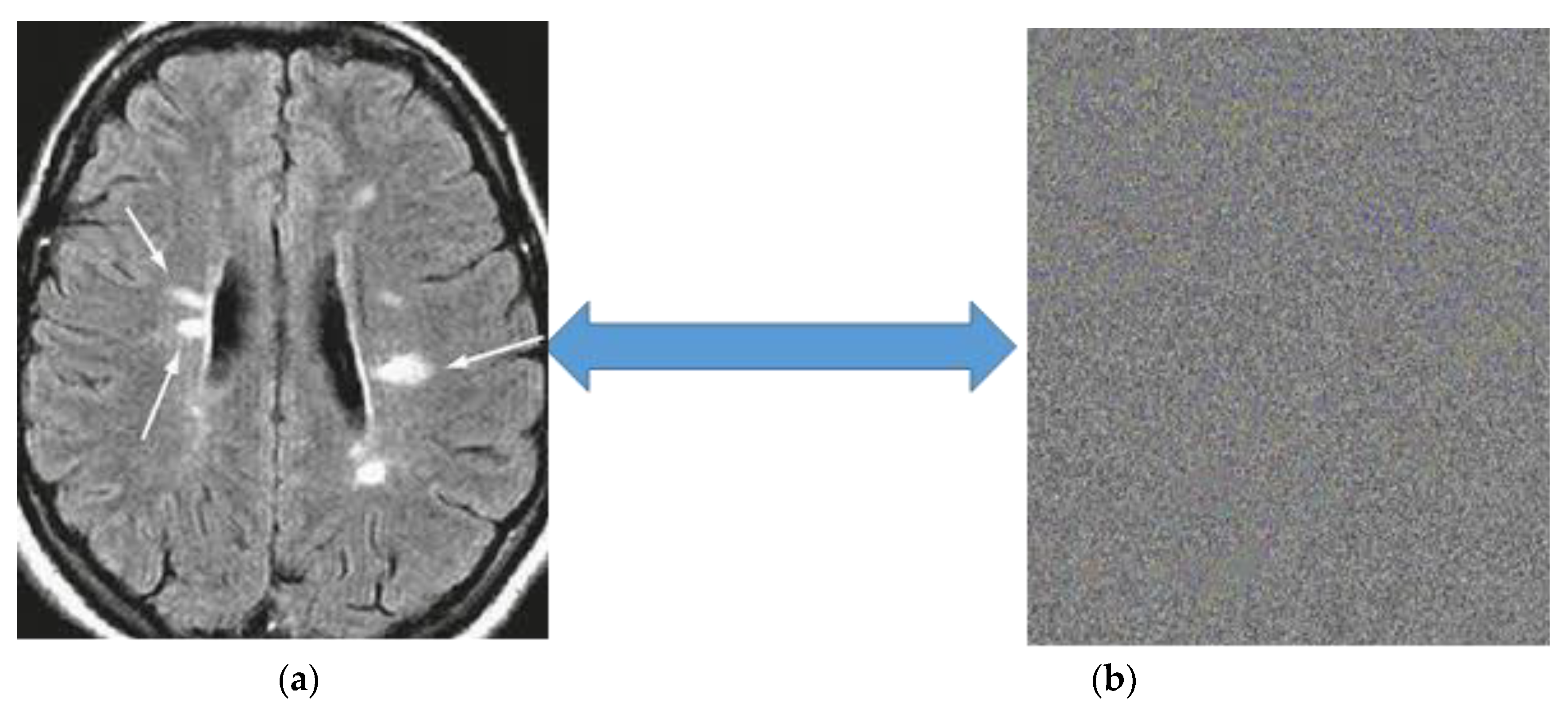
5.2.2. Cipher Image Analysis

Figure 9 indicates the plain normalized brain image and its corresponding encrypted image, otherwise called the cipher image. The analysis of the cipher image is based on only two metrics: the histogram and the correlation coefficient. For other metrics to evaluate an encryption algorithm’s efficiency, such as mean square error (MSE), peak signal-to-noise ratio (PSNR), and entropy, see the literature [22,26,78,79] for examples.

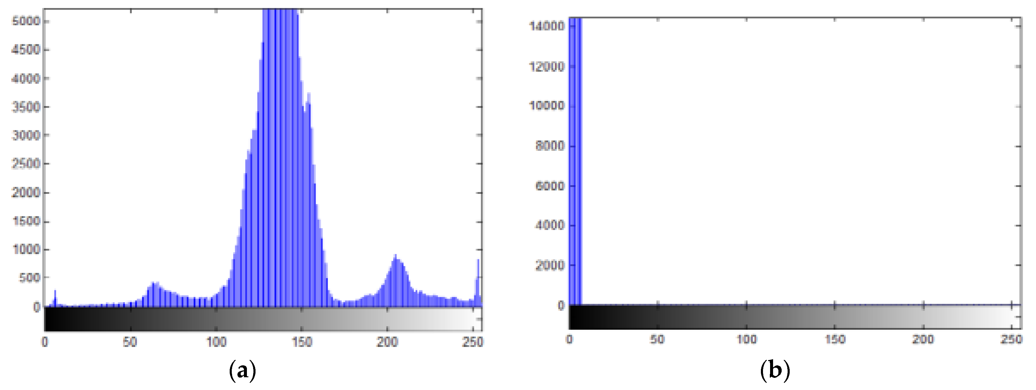
5.2.3. Histogram Analysis

The image histogram refers to a graph showing the number pixels in an image at each of the various intensity values present in the image. An image histogram, in other words, is a graphical representation of the distribution of pixel intensity in a grayscale or coloured image [80]. It is a pixel intensity plot against pixel count, where the x-axis indicates the gray level and the y-axis indicates the number of pixels. Figure 10 shows histograms of both a plain normalized brain image and its corresponding cipher image already shown in Figure 9. The histograms were generated using the ‘imhist’ function of MATLAB software. For analyzing the output of an encryption algorithm, similarity or otherwise in the histogram shapes between the plain image and its corresponding cypher image can be exploited. If these shapes are fully, somewhat, or partially similar, then the performance of an encryption algorithm is poor; otherwise, it is good. Clearly, different histogram shapes were returned for the plain brain image and its corresponding cipher image, hence encryption has taken place. We can, therefore, deduce that a successful encryption system was modelled for the normalized dyslexia-associated MRI dataset.

5.2.4. Correlation Coefficient Analysis

For determining the correlation coefficient between these images, the analysis of the intensity and direction of the relationship between adjacent pixels in both plain image and corresponding encrypted image may be used. By definition, the correlation coefficient (r) given in Equation (13) is the ratio of the covariance between the adjacent pixels in a plain and cipher image to the square root of the product of each of these pixels [81], where the value of r = −1 ≤ r ≤ 1 and r2 ≤ 1.
r = C o v ( x , y ) I p ( x ) I c ( y )
where x is a pixel from plain image and y is a pixel from the corresponding cipher image; and Ip and Ic are functions with a condition that, if r = 1, there is a strong direct or positive connection between the two pictures, which means there has been no encryption. If r = −1, however, the inverse or negative correlation is ideal, suggesting strong encryption. Further, r = 0 connotes that there is no linear correlation, however, there might be a non-linear correlation between the two images. Using Equation (13), the correlation coefficient between Figure 9a,b was found to be −0.0073. Meanwhile, to ensure poor correlation of all portions of our brain image dataset before classification, we obtain five randomly selection adjacent portions from Figure 9a,b for correlation analysis, as shown in Table 2. The purpose of this task is to ensure that the CNN classifier, which we assumed to be a cloud-based third party platform, does not gain partial access that may be used to guess the encoded information using the dictionary of known cipher-text attacks.
From the results presented in Table 2, we can conveniently conclude that our proposed pixel-bitstream encoder achieved better encryption with normalized brain images. While all other adjacent portions, including the whole image, showed negative correlation coefficient values, only adjacent portion 2 showed positive correlation coefficient value. Meanwhile, the value is insufficient and insignificant to gain partial access into that portion of the coded information.

5.3. Analysis of the Proposed Cascaded Deep CNN Classifier Performance

The proposed cascaded deep CNN classifier’s performance was quantitatively evaluated using deep model evaluation metrics based on stratified 10-fold cross validation (CV). These include the accuracy, sensitivity, specificity, and area under receiver operating characteristics (ROC) curve, each of which is derived directly from a confusion matrix (Figure 11) and defined in Equations (14)–(16). In particular, stratified 10-fold cross validation was chosen so that the average response value for all folds was approximately equal [12].
True positive (TP) is situation where the test dataset yields a correct or positive result for subjects with dyslexia, while true negative (TN) is a scenario when the test dataset yields a correct or negative output for subjects without dyslexia. All false positives (FP) and false negatives (FN) lead to errors of Type I and Type II, respectively.
  • Accuracy: Accuracy tests the percentage of dyslexic subjects correctly classified as positive. For computation of the classifier accuracy, Equation (14) is used.
    A c c u r a c y = T P + T N T P + T N + F P + F N
  • Sensitivity: Sensitivity is a measure of the percentage of dyslexic subjects that is correctly classified or predicted to be positive by the classifier. It is also known as the true positive rate (TPR) or recall. For the computation of sensitivity, Equation (15) is used.
    S e n s i t i v i t y = T P T P + F N
  • Specificity: Specificity, or the true negative rate (TNR), tests the percentage of correctly classified non-dyslexic subjects. This indicates accuracy in identifying non-dyslexic subjects [82], as shown in Equation (16).
    S p e c i f i c i t y = T N T N + F P
  • ROC and Area under ROC (AUC): The receiver operating characteristics (ROC) curve plots the sensitivity curve against specificity, and thus provides a representation of the trade-off between correctly classified positive instances and incorrectly classified negative instances [83]. Area under ROC (AUC) is computed directly from this curve.
To test the output of the proposed cascaded deep CNN as defined in Section 4.5, all 576,000 brain image patches were used. This sample comprises 243,200 with dyslexia biomarkers and 332,800 controls. The classification was made before and after pixel-bitstream encoding. To ensure that the proposed deep cascaded architecture learns pattens without compromising the privacy of the encrypted patches, the kernel size in the first pathway was reduced to 3 × 3 with a stride (2,2), while the kernel size in the second pathway was reduced to 7 × 7 with a stride (2,2). This arrangement allows augmentation to be performed on the encrypted data directly. In each case, 70% (403,200) of patches were used for training, 15% (86,400) of patches were used for each of the validation and testing, respectively. The experiment was simulated on MATLAB (R2017 b) software installed on a 2.70 GHz and 8.00 GB RAM GPU-based processor, at various training iterations: 150, 225, 350, 450, and 500 epochs, respectively. We decided to set a baseline of 50% accuracy level for the classification of the encrypted brain images owing to the disorganization of original pixels’ bitstream. Table 3 shows the summary of the classification results before and after encoding after 50 repeated stratified 10-fold CVs. The choice of our 50 runs for CV was intended to reduce the bias of the classifier (both overfitting and underfitting) and to minimize uncertainty, thus producing more reliable predictions.
From Table 3, the best training was achieved at 500 epochs iterations before and after encoding using pixel-bitstream encoder with the highest classification accuracy of 84.56% ± 4.91% and 73.19% ± 4.18%, respectively. However, the poor classification accuracy was observed at 150 epoch training iterations. Meanwhile, the classifier performed better than chance (50% baseline) before encoding, but poorly for the encoded images at the same iterations with a value 39.66% ± 2.09% which is significantly below the set baseline. This implies that, for the proposed cascaded deep CNN to reach promising performance of clinical relevance, the number of training iterations must be sufficiently large.
Expectedly, the classifier shows better accuracy, sensitivity, and specificity for image patches before encoding with the pixel-bitstream encoder, although the classifier still maintained good performance above chance in those metrics at the following iterations: 225, 350, 450, and 500, respectively. The reason for this may be the distortion in the pixels’ bits that represent the biomarkers under study, although the position of pixel collection representing biomarkers to be classified is conserved after RNS encryption. By extension, the classifier was able to learn these features. Advantageously, the concept of homomorphic encryption, which allows computations to be performed directly on the encrypted data, was successfully demonstrated. Figure 12 shows the ROC curve for the best training iteration after encoding. From this curve, the value of AUC is 0.76, which is significantly high.
Most of the biomarker features in this study that distinguish between dyslexic and control subjects can be found in the regions of gray matter (GM), white matter (WM), and cerebrospinal fluid (CSF), which constitute the brain’s phonological and cognitive sub-systems. By this, our results are consistent with those of Tamboer et al. [11], Cui et al. [84], and Sarah et al. [85]. Although Plonski et al. [12] and Plonski et al. [52] have argued that discriminating dyslexia biomarker features are traceable to the geometric properties of the human brain cortex, this study does not consider the geometric properties of cerebral cortex during the feature extraction stage.
While existing machine learning algorithms such as artificial neural network (ANN), support vector machine (SVM), and K-nearest neighbour (K-NN) used by earlier studies relied on error-prone, time-consuming, hand-crafted features selection mechanisms to discriminate between the dyslexic group and normal subjects, cascaded deep CNN extracts high-level features directly from the given dataset. Hence, this study corroborates Spoon et al.’s [86] research by illustrating the use of a deep learning algorithm to classify learning disability. We also clearly demonstrated the possibility of distinguishing biomarkers of dyslexia from an encrypted MRI dataset—a concept we described as CryptoDL. Meanwhile, we found that larger percentage of developmental dyslexia classification studies, particularly machine learning algorithms, assessing classifier performance based on accuracy, sensitivity, and specificity metrics only. These metrics are not sufficient. For instance, accuracy, which is the most frequently used, becomes subject to bias in a situation of missing values or when one of the classes to be predicted over-dominates the dataset that is, imbalanced class distribution [87,88]. This kind of scenario is inevitable when analyzing data relating to learning disability, hence the need for more sophisticated evaluation metrics.
The proposed approach is compared against three recent studies based on privacy-preservation classification with homomorphic encryption, and the performance is shown in Table 4. All the deep learning classifiers used, including the proposed cascaded deep CNN, are shown to be above the baseline of 50% performance accuracy on the encrypted image datasets. The highest classification accuracy was achieved by Sirichotedumrong et al. [35], with an accuracy of 86.99%, while the lowest classification accuracy was achieved by Tanaka [89], with an accuracy of 56.80%. The reason for this is associated with overlapping of the classifier’s block of adaptation layers with the adjacent encrypted block from the type of image encryption algorithm adopted. All pixel-based algorithms, including the proposed approach, show relatively high performance accuracies, as the location of pixel collections representing important features or biomarkers in the image is conserved regardless of the fact that the bitstream has been modified for each pixel. Compared with the Chao et al. method [25], our proposed method performs better as a result of a very high computational complexity of polynomial activation function, which limits the computable depth of multiplication capability.
Finally, owing to the computational overhead of the large numbers of parameters used, our proposed approach performs comparatively inferior to that of Sirichotedumrong et al. [35]. Therefore, approaches to tackle the optimization of parameters for the proposed cascaded deep CNN represent a subject for potential investigation.

5.4. Summary of Discussion

The RNS encryption scheme used to build the pixel-bitstream encoder is a pixel-based encryption scheme that allows the proposed cascaded deep CNN classifier to learn features over the encrypted training neuroimaging dataset and to predict dyslexia cases using the encrypted test dataset. The outcomes of the classification are also in encoded form. The RNS-based encryption scheme is homomorphic in terms of arbitrary addition, subtraction, and multiplication operations that could be performed directly without decrypting the data. Both theoretical architectural analysis and FPGA implementation of our proposed pixel-bitstream encoder showed that, after encoding, the location of the array of pixels representing a particular biomarker of dyslexia is preserved. Consequently, the design has helped the proposed deep CNN classifier to achieve reasonably high accuracy, sensitivity, and specificity, as illustrated in Table 3.
Evidence from histograms and correlation analyses shows that the proposed pixel-bitstream encoder architecture implemented on a pure adder-based FPGA is not only time-efficient, but also enhances the encoding of clearly defined neuroimaging datasets into their corresponding cipher images. It is also evident from our study that classification accuracy is proportional to the number of training iterations (epochs) for the encrypted dataset, implying that the proposed cascaded deep CNN better learns appropriate encrypted biomarkers (features) with the increasing number of training cycles. Meanwhile, in accordance with earlier studies [11,12,52,84] on the classification of developmental dyslexia using machine learning techniques, our report also asserts that volumetric and geometric properties of essential tissues in the brain’s phonological and cognitive sub-systems constitute distinguishing variables for dyslexia cases with or without data encryption.

6. Conclusions

In this study, we suggest a method for the safe detection of biomarkers for dyslexia from brain MRI datasets (neuroimaging dataset). Our approach utilized an RNS special moduli set to design an adder-based, pixel-bitstream encoder to convert a 7-bit grayscale normalized dyslexia biomarkers-associated image dataset to cipher images before subjecting them to deep learning using cascaded deep convolutional neural network. Theoretically, we were able to show that the proposed pixel-bitstream encoder has an area complexity of 4n AFA and a total time delay of (3n + 3) DFA when the value of n ≥ 3. FPGA implementation of the proposed encoder revealed that the encoder was able to save up to 42.4% energy compared with ROM-based implementation, with a decrease in critical path delay value of 23.5% compared with the state-of-the-art binary-to-residue converter equivalent. When used for the encryption process, the proposed encoder achieved approximately 15 s time for the creation of cipher images for all image patches segmented during the pre-processing phase. The correlation between the plain normalized brain and cipher images was found to range between −0.0073 and 0.0082 with completely different histogram shapes.
The analysis of the proposed cascaded deep CNN classifier shows that efficient classification results can be achieved without revealing the secret of the dataset used. This supports the existing concept of CryptoNets, a situation where machine learning or deep learning algorithms are specifically applied to encrypted data [20,24], and privacy-preserving classification based on homomorphic cryptosystem [19,88]. Although our results have shown better classification outcomes without encoding the dataset, optimal accuracy and better prediction output can be achieved when the number of training iterations is sufficiently large, with or without encoding the image patches. This should be accompanied by careful selection of other deep model parameters.
In the meantime, the dyslexia-related dataset was chosen for our analysis owing to the effects of dyslexia on the victim individual’s life and culture as a whole. Future work should concentrate on the analysis of the proposed classifier using more sophisticated metrics. Further, evaluating the homomorphic capability and asymptotic efficiency of the proposed pixel-bitstream encoder will be an added advantage.

Author Contributions

Conceptualization, O.L.U.; Methodology, O.L.U. and R.C.M.; Software, O.L.U.; Validation, O.L.U. and R.C.M.; Formal Analysis, R.C.M.; Investigation, O.L.U.; Resources, O.L.U. and R.C.M.; Data Curation, O.L.U.; Writing—Original Draft Preparation, O.L.U.; Writing—Review and Editing, R.C.M.; Visualization, O.L.U.; Supervision, R.C.M.; Project Administration, R.C.M.; Funding Acquisition, R.C.M. All authors have read and agreed to the published version of the manuscript.

Funding

This research is funded by Universiti Kebangsaan Malaysia (UKM), UKM Grant Code: GGP-2019-023.

Conflicts of Interest

The authors declare that there is no conflict of interest.

References

  1. Shen, D.; Wu, G.; Suk, H. Deep Learning in Medical Image Analysis. Annu. Rev. Biomed. Eng. 2017, 19, 221–248. [Google Scholar] [CrossRef] [PubMed] [Green Version]
  2. Biomarker Working Group. Biomarkers and surrogate endpoints: Preferred definitions and conceptual framework. Clin. Pharmacol. Ther. 2001, 69, 89–95. [Google Scholar]
  3. Sharin, U.; Abdullah, S.N.H.S.; Omar, K.; Adam, A.; Sharis, S. Prostate Cancer Classification Technique on Pelvis CT Images. Int. J. Eng. Technol. 2019, 8, 206–213. [Google Scholar]
  4. Lundervold, A.S.; Lundervold, A. An overview of deep learning in medical imaging focusing on MRI. Z. Med. Phys. 2019, 29, 102–127. [Google Scholar] [CrossRef] [PubMed]
  5. Elnakib, A.; Soliman, A.; Nitzken, M.; Casanova, M.F.; Gimel’farb, G.; El-Baz, A. Magnetic resonance imaging findings for dyslexia: A review. J. Biomed. Nanotechnol. 2014, 10, 2778–2805. [Google Scholar] [CrossRef] [PubMed]
  6. Sun, Y.F.; Lee, J.S.; Kirby, R. Brain imaging findings in dyslexia. Pediatr. Neonatol. 2010, 51, 89–96. [Google Scholar] [CrossRef] [Green Version]
  7. Casanova, M.F.; El-Baz, A.; Elnakib, A.; Giedd, J.; Rumsey, J.M.; Williams, E.L.; Andrew, E.S. Corpus callosum shape analysis with application to dyslexia. Transl. Neurosci. 2010, 1, 124–130. [Google Scholar] [CrossRef]
  8. Farr, L.; Mancho-For, N.; Montal, M. Estimation of Brain Functional Connectivity in Patients with Mild Cognitive Impairment. Brain Sci. 2019, 9, 350. [Google Scholar] [CrossRef] [Green Version]
  9. Wajuihian, S.O.; Naidoo, K.S. Dyslexia: An overview. Afr. Vis. Eye Health 2011, 70, 89–98. [Google Scholar] [CrossRef] [Green Version]
  10. Yuzaidey, N.A.M.; Din, N.C.; Ahmad, M.; Ibrahim, N.; Razak, R.A.; Harun, D. Interventions for children with dyslexia: A review on current intervention methods. Med. J. Malays. 2018, 73, 311–320. [Google Scholar]
  11. Tamboer, P.; Vorst, H.C.M.; Ghebreab, S.; Scholte, H.S. Machine learning and dyslexia: Classification of individual structural neuro-imaging scans of students with and without dyslexia. NeuroImage Clin. 2016, 11, 508–514. [Google Scholar] [CrossRef] [PubMed] [Green Version]
  12. Płoński, P.; Gradkowski, W.; Altarelli, I.; Monzalvo, K.; van Ermingen-Marbach, M.; Grande, M.; Hein, S.; Marchewka, A.; Bogorodzki, P.; Ramus, F.; et al. Multi-parameter machine learning approach to the neuroanatomical basis of developmental dyslexia. Hum. Brain Mapp. 2017, 38, 900–908. [Google Scholar] [CrossRef] [PubMed]
  13. Ravi, D.; Wong, C.; Deligianni, F.; Berthelot, M.; Andreu-Perez, J.; Lo, B.; Yang, G.-Z. Deep Learning for Health Informatics. IEEE J. Biomed. Health Inform. 2017, 21, 4–21. [Google Scholar] [CrossRef] [PubMed] [Green Version]
  14. Dash, S.; Acharya, B.R.; Mittal, M.; Ajith, A.; Kelemen, A. Deep Learning Techniques for Biomedical and Health Informatics; Springer: Berlin/Heidelberg, Germany, 2020. [Google Scholar]
  15. Yu, L.; Chen, H.; Dou, Q.; Qin, J.; Heng, P.A. Integrating Online and Offline 3D Deep Learning for Automated Polyp Detection in Colonoscopy Videos. IEEE J. Biomed. Health Inform. 2016, 2194, 1–11. [Google Scholar]
  16. Oyedotun, O.K.; Olaniyi, E.O. Deep Learning in Character Recognition Considering Pattern Invariance Constraints. Int. J. Syst. Appl. 2015, 7, 1–10. [Google Scholar] [CrossRef] [Green Version]
  17. Russakovsky, O.; Deng, J.; Su, H.; Krause, J.; Satheesh, S.; Ma, S.; Huang, Z.; Karpathy, A.; Khosla, A.; Bernstein, M.; et al. ImageNet Large Scale Visual Recognition Challenge. Int. J. Comput. Vis. 2015, 115, 211–252. [Google Scholar] [CrossRef] [Green Version]
  18. Ren, J. Investigation of Convolutional Neural Network Architectures for Image-based Feature Learning and Classification; University of Washington: Bothell, WA, USA, 2016. [Google Scholar]
  19. Zhu, Q.; Lv, X. 2P-DNN: Privacy-Preserving Deep Neural Networks Based on Homomorphic Cryptosystem. arXiv 2018, arXiv:1807.08459. [Google Scholar]
  20. Pengtao, X.; Bilenko, M.; Finley, T.; Gilad-Bachrach, R.; Lauter, K.; Naehrig, M. Crypto-Nets: Neural Networks over Encrypted Data. arXiv 2014, arXiv:1412.6181. [Google Scholar]
  21. Mahmood, A.; Hamed, T.; Obimbo, C.; Dony, R. Improving the Security of the Medical Images. Int. J. Adv. Comput. Sci. Appl. 2013, 4, 137–146. [Google Scholar] [CrossRef] [Green Version]
  22. Al-Haj, A.; Abandah, G.; Hussein, N. Crypto-based algorithms for secured medical image transmission. IET Inf. Secur. 2015, 9, 365–373. [Google Scholar] [CrossRef]
  23. Gatta, M.T.; Al-Latief, S.T.A. Medical image security using modified chaos-based cryptography approach. J. Phys. Conf. Ser. 2018, 1003, 1–6. [Google Scholar] [CrossRef]
  24. Dowlin, N.; Gilad-Bachrach, R.; Laine, K.; Lauter, K.; Naehrig, M.; Wernsing, J. CryptoNets: Applying neural networks to Encrypted data with high throughput and accuracy—Microsoft research. In Proceedings of the 33rd International Conference on Machine Learning, New York, NY, USA, 24 February 2016; pp. 1–12. [Google Scholar]
  25. Chao, J.; Badawi, A.A.; Unnikrishnan, B.; Lin, J.; Mun, C.F.; Brown, J.M.; Campbell, J.P.; Chiang, M.; Kalpathy-Cramer, J.; Chandrasekhar, V.R.; et al. CaRENets: Compact and Resource-Efficient CNN for Homomorphic Inference on Encrypted Medical Images. arXiv 2019, arXiv:1901.10074. [Google Scholar]
  26. Koppu, S.; Viswanatham, V.M. A Fast Enhanced Secure Image Chaotic Cryptosystem Based on Hybrid Chaotic Magic Transform. Model. Simul. Eng. 2017, 2017, 1–13. [Google Scholar] [CrossRef] [Green Version]
  27. Zhu, C.; Wang, G.; Sun, K. Cryptanalysis and Improvement on an Image Encryption Algorithm Design Using a Novel Chaos Based S-Box. Symmetry 2018, 10, 399. [Google Scholar] [CrossRef] [Green Version]
  28. Safari, A.; Kong, Y. Four tap Daubechies filter banks based on RNS. In Proceedings of the IEEE 2012 International Symposium on Communications and Information Technologies (ISCIT), Gold Coast, QLD, Australia, 2–5 October 2012; pp. 952–955. [Google Scholar]
  29. Bankas, E.K.; Gbolagade, K.A. A New Efficient RNS Reverse Converter for the 4-Moduli Set. Int. J. Comput. Electr. Autom. Control Inf. Eng. 2014, 8, 328–332. [Google Scholar]
  30. Navin, A.H.; Oskuei, A.R.; Khashandarag, A.S.; Mirnia, M. A Novel Approach Cryptography by using Residue Number System. In Proceedings of the ICCIT, 6th International Conference on Computer Science and Convergence Information Technology IEEE, Seogwipo, Korea, 29 November–1 December 2011. [Google Scholar]
  31. Abdul-mumin, S.; Gbolagade, K.A. Mixed Radix Conversion based RSA Encryption System. Int. J. Comput. Appl. 2016, 150, 43–47. [Google Scholar] [CrossRef]
  32. Alhassan, S.; Gbolagade, K.A. Enhancement of the Security of a Digital Image using the Moduli Set. J. Adv. Res. Comput. Eng. Technol. 2013, 2, 2223–2229. [Google Scholar]
  33. Youssef, M.I.; Eman, A.E.; Elghany, M.A. Multi-Layer Data Encryption using Residue Number System in DNA Sequence. Int. J. Comput. Appl. 2012, 45, 19–24. [Google Scholar]
  34. Youssef, M.I.; Emam, A.E.; Saafan, S.M.; Elghany, M.A.B.D. Secured Image Encryption Scheme Using both Residue Number System and DNA Sequence. Online J. Electron. Electr. 2013, 6, 656–664. [Google Scholar]
  35. Sirichotedumrong, W.; Maekawa, T.; Kinoshita, Y.; Kiya, H. Privacy-Preserving Deep Neural Networks with Pixel-based Image Encryption Considering Data Augmentation in the Encrypted Domain. In Proceedings of the IEEE International Conference on Image Processing, Taipei, Taiwan, 22–25 September 2019; pp. 1–5. [Google Scholar]
  36. Liu, X.; Zou, Y.; Kuang, H.; Ma, X. Face Image Age Estimation Based on Data Augmentation and Lightweight Convolutional. Symmetry 2020, 12, 146. [Google Scholar] [CrossRef] [Green Version]
  37. Fukushima, K. Neocognition: A self. Biol. Cybern. 1980, 202, 193–202. [Google Scholar] [CrossRef]
  38. Yadav, S.S.; Jadhav, S.M. Deep convolutional neural network based medical image classification for disease diagnosis. J. Big Data 2019, 6, 1–18. [Google Scholar] [CrossRef] [Green Version]
  39. Lecun, Y.; Bengio, Y.; Hinton, G. Deep learning. Nature 2015, 521, 436–444. [Google Scholar] [CrossRef] [PubMed]
  40. Khan, A.; Sohail, A.; Zahoora, U.; Qureshi, A.S. A Survey of the Recent Architectures of Deep Convolutional Neural Networks. arXiv 2019, arXiv:1901.06032. [Google Scholar] [CrossRef] [Green Version]
  41. Khan, A.; Sohail, A.; Ali, A. A New Channel Boosted Convolutional Neural Network using Transfer Learning. arXiv 2018, arXiv:1804.08528. [Google Scholar]
  42. Rahman, A.; Muniyandi, R.C. An Enhancement in Cancer Classification Accuracy Using a Two-Step Feature Selection Method Based on Artificial Neural Networks with 15 Neurons. Symmetry 2020, 12, 271. [Google Scholar] [CrossRef] [Green Version]
  43. Niethammer, M.; Styner, M.; Aylward, S.; Zhu, H.; Oguz, I.; Yap, P.-T.; Shen, D. Information Processing in Medical Imaging. In Proceedings of 25th International Conference, IPMI 2017; Hutchison, D., Ed.; Springer: Boone, NC, USA, 2017. [Google Scholar]
  44. Cole, J.H.; Poudel, R.P.K.; Tsagkrasoulis, D.; Caan, M.W.A.; Steves, C.; Spector, T.D.; Montana, G. Predicting brain age with deep learning from raw imaging data results in a reliable and heritable biomarker. Neuroimage 2017, 1–25. [Google Scholar] [CrossRef] [Green Version]
  45. Hesamifard, E.; Takabi, H.; Ghasemi, M. CryptoDL: Deep Neural Networks over Encrypted Data. arXiv 2017, arXiv:1711.05189. [Google Scholar]
  46. Chervyakov, N.I.; Lyakhov, P.A.; Valueva, M.V.; Valuev, G.V.; Kaplun, D.I.; Efimenko, G.A.; Gnezdilov, D.V. Area-Efficient FPGA Implementation of Minimalistic Convolutional Neural Network Using Residue Number System. In Proceedings of the IEEE 23rd Conference of Frust Association, Bologna, Italy, 13–16 November 2018; pp. 112–118. [Google Scholar]
  47. Dimauro, G.; Impedovo, S.; Pirlo, G. A New Technique for Fast Number Comparison in the Residue Number System. IEEE Trans. Comput. 1993, 42, 608–612. [Google Scholar] [CrossRef]
  48. Gbolagade, K.A.; Cotofana, S.D. An O(n) Residue Number System to Mixed Radix Conversion Technique. In Proceedings of the IEEE Conference on Very Large Scale Integration, Taipei, Taiwan, 24–27 May 2009; pp. 521–524. [Google Scholar]
  49. Abdul-mumin, S.; Gbolagade, K.A. An Improved Residue Number System Based RSA Cryptosystem. Int. J. Emerg. Technol. Comput. Appl. Sci. 2017, 20, 70–74. [Google Scholar]
  50. Lotfinejad, M.M.; Mosleh, M.; Noori, H. A novel generic three-moduli set and its optimum arithmetic residue to binary converters. In Proceedings of the 2010 the 2nd International Conference on Computer and Automation Engineering (ICCAE), Singapore, 26–29 February 2010; pp. 112–116. [Google Scholar]
  51. Cao, B.; Srikanthan, T.; Chang, C.H. Design of residue-to-binary converter for a new 5-moduli superset residue number system. In Proceedings of the 2004 IEEE International Symposium on Circuits and Systems, Vancouver, BC, Canada, 23–26 May 2004. [Google Scholar]
  52. Płoński, P.; Gradkowski, W.; Marchewka, A.; Jednoróg, K.; Bogorodzki, P. Dealing with the heterogeneous multi-site neuroimaging data sets: A discrimination study of children dyslexia. In Brain Informatics and Health. BIH 2014, Lecture Notes in Computer Science, 8609; Ślȩzak, D., Tan, A.H., Peters, J.F., Schwabe, L., Eds.; Springer: Cham, Switzerland, 2014. [Google Scholar]
  53. Dale, A.M.; Fischl, B.; Sereno, M.I. Cortical Surface-Based Analysis: I. Segmentation and Surface Reconstruction. Neuroimage 1999, 9, 179–194. [Google Scholar] [CrossRef]
  54. Sun, X.; Shi, L.; Luo, Y.; Yang, W.; Li, H.; Liang, P.; Li, K.; Mok, V.C.T.; Chu, W.C.W.; Wang, D. Histogram—Based normalization technique on human brain magnetic resonance images from different acquisitions. Biomed. Eng. Online 2015, 14, 1–17. [Google Scholar] [CrossRef] [PubMed] [Green Version]
  55. Kleesiek, J.; Urban, G.; Hubert, A.; Schwarz, D.; Maier-Hein, K.; Bendszus, M.; Briller, A. Neuroimage Deep MRI brain extraction: A 3D convolutional neural network for skull stripping. Neuroimage 2016, 129, 460–469. [Google Scholar] [CrossRef] [PubMed]
  56. Im, K.; Raschle, N.M.; Smith, S.A.; Ellen, G.P.; Gaab, N. Atypical Sulcal Pattern in Children with Developmental Dyslexia and At-Risk Kindergarteners. Cereb. Cortex 2016, 26, 1138–1148. [Google Scholar] [CrossRef] [PubMed] [Green Version]
  57. Tamboer, P.; Scholte, H.S.; Vorst, H.C.M. Dyslexia and voxel-based morphometry: Correlations between five behavioural measures of dyslexia and gray and white matter volumes. Ann. Dyslexia 2015, 65, 121–141. [Google Scholar] [CrossRef] [Green Version]
  58. Zhang, L.; Wang, X.; Penwarden, N.; Ji, Q. An Image Segmentation Framework Based on Patch Segmentation Fusion. In Proceedings of the 18th International Conference on Pattern Recognition (ICPR’06), Hong Kong, China, 20–24 August 2006; pp. 1–5. [Google Scholar]
  59. Alkinani, M.H.; El-Sakka, M.R. Patch-based models and algorithms for image denoising: A comparative review between patch-based images denoising methods for additive noise reduction. EURASIP J. Image Video Process. 2017, 58, 1–27. [Google Scholar] [CrossRef]
  60. Parhami, B. Digital/analog arithmetic with continuous-valued residues. In Proceedings of the 2009 Conference Record of the Forty-Third Asilomar Conference on Signals, Systems and Computers, Pacific Grove, CA, USA, 1–4 November 2009. [Google Scholar]
  61. Omondi, A.; Premkumar, B. Residue Number Systems: Theory and Implementation. In Covent Garden, London; Imperial College Press: London, UK, 2007. [Google Scholar]
  62. Jaberipur, G.; Belghadr, A.; Nejati, S. Impact of diminished-1 encoding on residue number systems arithmetic units and converters. Comput. Electr. Eng. 2019, 75, 61–76. [Google Scholar] [CrossRef]
  63. Shin, H.; Roth, H.R.; Gao, M.; Lu, L.; Xu, Z.; Nogues, I.; Yao, J.; Mollura, D.; Summers, R.M. Deep Convolutional Neural Networks for Computer-Aided Detection: CNN Architectures, Dataset Characteristics and Transfer Learning. IEEE Trans. Med. Imaging 2016, 35, 1285–1298. [Google Scholar] [CrossRef] [Green Version]
  64. Kafi, M.; Maleki, M.; Davoodian, N. Research in Veterinary Science Functional histology of the ovarian follicles as determined by follicular fluid concentrations of steroids and IGF-1 in Camelus dromedarius. Res. Vet. Sci. 2015, 99, 37–40. [Google Scholar] [CrossRef]
  65. Bengio, Y. Deep Learning of Representations: Looking Forward. In Statistical Language and Speech Processing. SLSP 2013, Lecture Notes in Computer Science, 7978; Dediu, A.H., Martín-Vide, C., Mitkov, R., Truthe, B., Eds.; Springer: Berlin/Heidelberg, Germany, 2013. [Google Scholar]
  66. Nguyen, Q.; Mukkamala, M.C.; Hein, M. Neural Networks Should be Wide Enough to Learn Disconnected Decision Regions. arXiv 2018, arXiv:1803.00094. [Google Scholar]
  67. Havaei, M.; Davy, A.; Warde-Farley, D.; Biard, A.; Courville, A.; Bengio, Y.; Pal, C.; Jodoin, P.; Larochelle, H. Brain Tumor Segmentation with Deep Neural Networks. Med. Image Anal. 2017, 35, 18–31. [Google Scholar] [CrossRef] [Green Version]
  68. Kamnitsas, K.; Ledig, C.; Newcombe, V.F.J.; Simpson, J.P.; Kane, A.D.; Menon, D.K.; Rueckert, D.; Glocker, B. Efficient multi-scale 3D CNN with fully connected CRF for accurate brain lesion segmentation. Med. Image Anal. 2017, 36, 61–78. [Google Scholar] [CrossRef]
  69. Dou, Q.; Chen, H.; Yu, L.; Zhao, L.; Qin, J.; Wang, D.; Mok, V.C.T.; Shi, L.; Heng, P. Automatic Detection of Cerebral Microbleeds from MR Images via 3D Convolutional Neural Networks. IEEE Trans. Med. Imaging 2016, 35, 1182–1195. [Google Scholar] [CrossRef]
  70. Dou, Q.; Yu, L.; Chen, H.; Jin, Y.; Yang, X.; Qin, J.; Heng, P. 3D deeply supervised network for automated segmentation of volumetric medical images. Med. Image Anal. 2017, 41, 40–54. [Google Scholar] [CrossRef] [PubMed]
  71. Payan, A.; Montana, G. Predicting Alzheimer’s disease: A neuroimaging study with 3D convolutional neural networks. arXiv 2015, arXiv:1502.02506. [Google Scholar]
  72. Amerineni, R.; Gupta, R.S.; Gupta, L. CINET: A Brain-Inspired Deep Learning Context—Integrating Neural Network Model for Resolving Ambiguous Stimuli. Brain Sci. 2020, 10, 64. [Google Scholar] [CrossRef] [PubMed] [Green Version]
  73. Srivastava, N.; Hinton, G.; Krizhevsky, A.; Sutskever, I.; Salakhutdinov, R. Dropout: A Simple Way to Prevent Neural Networks from Overfitting. J. Mach. Learn. Res. 2014, 15, 1929–1958. [Google Scholar]
  74. Krizhevsky, A.; Sustskever, I.; Hinton, G. ImageNet Classification with Deep Convolutional Neural Networks. Commun. ACM 2017, 84–90. [Google Scholar] [CrossRef]
  75. Zeiler, M.D.; Fergus, R. Visualizing and understanding convolutional networks. In Computer Vision – ECCV 2014. Lecture Notes in Computer Science, 8689; Fleet, D., Pajdla, T., Schiele, B., Tuytelaars, T., Eds.; Springer: Cham, Germany.
  76. Maroosi, A.; Muniyandi, R.C. Accelerated Execution of P Systems with Active Membranes to solve the N-Queens Problem. Theor. Comput. Sci. 2014, 551, 39–54. [Google Scholar]
  77. Maroosi, A.; Muniyandi, R.C.; Sundararajan, E.; Zin, A.M. Parallel and Distributed Computing Models on a Graphics Processing Unit to Accelerate Simulation of Membrane Systems. Stimul. Model. Pract. Theory 2014, 47, 60–78. [Google Scholar]
  78. Othman, A.; Muniyandi, R.C. Elliptic Curve Diffie-Hellman Random Keys Using Artificial Neural Network and Genetic Algorithm for Secure Data over Private Cloud. Inf. Technol. J. 2016, 15, 77–83. [Google Scholar] [CrossRef] [Green Version]
  79. Zhou, Y.; Panetta, K.; Agaian, S. An image scrambling algorithm using parameter based M-sequences. In Proceedings of the 2008 International Conference on Machine Learning and Cybernetics, Kunming, China, 12–15 July 2008. [Google Scholar]
  80. Somaraj, S.; Hussain, M.A. A Novel Image Encryption Technique Using RGB Pixel Displacement for Color Images. In Proceedings of the 2016 IEEE 6th International Conference on Advanced Computing (IACC), Bhimavaram, India, 27–28 February 2016. [Google Scholar]
  81. Wang, Y.; Wong, K.W.; Liao, X.; Xiang, T.; Chen, G. A chaos-based image encryption algorithm with variable control parameters. Chaos Solitons Fractals 2009, 41, 1773–1783. [Google Scholar] [CrossRef]
  82. Macaš, M.; Novak, D.; Kordik, P.; Lhotska, L.; Vyhnalek, M.; Brzezny, R. Dyslexia Detection from Eye Movements Using Artificial Neural Networks. In Proceedings of the European Medical and Biological Engineering Conference, Prague, Czech Republic, 20–25 November 2005; pp. 1–10. [Google Scholar]
  83. Buda, M.; Maki, A.; Mazurowski, M.A. A systematic study of the class imbalance problem in convolutional neural networks. Neural Netw. 2018, 106, 249–259. [Google Scholar] [CrossRef] [PubMed] [Green Version]
  84. Cui, Z.; Xia, Z.; Su, M.; Shu, H.; Gong, G. Disrupted white matter connectivity underlying developmental dyslexia: A machine learning approach. Hum. Brain Mapp. 2016, 37, 1443–1458. [Google Scholar] [CrossRef] [PubMed]
  85. Sarah, B.; Nicole, C.; Ardag, H.; Madelyn, M.; Holland, S.K.; Tzipi, H. An fMRI Study of a Dyslexia Biomarker. J. Young Investig. 2014, 26, 1–4. [Google Scholar]
  86. Spoon, K.; Crandall, D.; Siek, K. Towards Detecting Dyslexia in Children’s Handwriting Using Neural Networks. In Proceedings of the International Conference on Machine Learning AI for Social Good Workshop, Long Beach, CA, USA, 15 June 2019; pp. 1–5. [Google Scholar]
  87. Johnson, J.M.; Khoshgoftaar, T.M. Survey on deep learning with class imbalance. J. Big Data 2019, 6, 1–54. [Google Scholar] [CrossRef]
  88. Bost, R.; Popa, R.A.; Tu, S.; Goldwasser, S. Machine Learning Classification over Encrypted Data. In Proceedings of the NDSS Conference, San Diego, CA, USA, 8–11 February 2015; pp. 1–14. [Google Scholar]
  89. Tanaka, M. Learnable Image Encryption. In Proceedings of the IEEE International Conference on Consumer Electronics-Taiwan (ICCE-TW), Taichung, Taiwan, 19–21 May 2018; pp. 1–2. [Google Scholar]
Figure 1. Feature maps extraction [46].
Symmetry 12 00836 g001
Figure 2. Max-pooling operation.
Symmetry 12 00836 g002
Figure 3. Simplified deep convolutional neural network architecture [4].
Symmetry 12 00836 g003
Figure 4. Proposed conceptual framework. RNS, residue number system; CNN, convolutional neural network.
Symmetry 12 00836 g004
Figure 5. General architecture of RNS encoder.
Symmetry 12 00836 g005
Figure 6. Hardware design of pixel encoder. CSA, carry save adder; CPA, carry propagate adder.
Symmetry 12 00836 g006
Figure 7. Cascaded deep CNN architecture.
Symmetry 12 00836 g007
Figure 8. Encoding time for patches in seconds.
Symmetry 12 00836 g008
Figure 9. Plain image and cipher image comparison: (a) plain brain image and (b) cipher image.
Symmetry 12 00836 g009
Figure 10. Comparison of histograms: (a) plain brain image and (b) cipher image.
Symmetry 12 00836 g010
Figure 11. Confusion matrix.
Symmetry 12 00836 g011
Figure 12. Receiver operating characteristics (ROC) curve at a training iteration of 500 epochs after encoding. AUC, area under ROC.
Symmetry 12 00836 g012
Table 1. Critical path delay of the proposed converter.
Virtex-4 FPGA Delay in SecondsSpartan-3 FPGA Delay in Seconds
nCritical Path (2n+1 − 1)Proposed EncoderState-of-the-Art (2)% ImprovementProposed EncoderState-of-the-Art (2)% Improvement
425 − 123.725.67.425.530.115.3
526 − 129.933.711.335.239.711.3
829 − 137.148.523.5---
11212 − 156.868.316.8---
Table 2. Summary of correlation analysis.
Adjacent PortionsCorrelation Coefficient (r)
Portion1−0.0293
Portion20.0082
Portion3−0.0275
Portion4−0.0111
Portion5−0.0659
Whole Images−0.0073
Table 3. Classification results before and after encoding (mean ± SD after 50 repeated 10-fold cross validation (CV)).
Before EncodingAfter Encoding
Training IterationsAccuracy (%)Sensitivity (%)Specificity (%)Accuracy (%)Sensitivity (%)Specificity (%)
15057.47 ± 2.5840.19 ± 2.1353.62 ± 2.3339.66 ± 2.0933.28 ± 2.5137.18 ± 2.85
22559.13 ± 3.7661.23 ± 3.7254.91 ± 3.1958.39 ± 3.4458.72 ± 3.0653.31 ± 3.41
35070.68 ± 4.0265.29 ± 2.9766.84 ± 2.8863.42 ± 3.1961.97 ± 2.8962.00 ± 2.99
45080.22 ± 4.4671.33 ± 3.8572.53 ± 4.1268.99 ± 3.8767.81 ± 4.7368.03 ± 3.96
50084.56 ± 4.9176.25 ± 4.6478.21 ± 4.3373.19 ± 4.1870.33 ± 4.4671.43 ± 4.11
Table 4. Performance comparison with existing privacy-preservation methods. MRI, magnetic resonance imaging; CNN, convolutional neural network.
Author(s) and YearImage Encrypted AlgorithmDeep Learning Classifier UsedSource of Dataset UsedAccuracy (%)Reference No.
Tanaka (2018)Block-basedPyramidal Residue NetworkCIFER Dataset56.80[89]
Sirichotedumrong et al. (2019)Pixel-basedResNet-18CIFER Dataset86.99[35]
Chao et al. (2019)-CaRENetsMNIST Dataset73.10[25]
Proposed Pixel-basedTwo-Pathway Cascaded Deep CNNKaggle Brain MRI Dataset73.19-

