Malware Classification Using Simhash Encoding and PCA (MCSP)

Abstract

Malware is any malicious program that can attack the security of other computer systems for various purposes. The threat of malware has significantly increased in recent years. To protect our computer systems, we need to analyze an executable file to decide whether it is malicious or not. In this paper, we propose two malware classification methods: malware classification using Simhash and PCA (MCSP), and malware classification using Simhash and linear transform (MCSLT). PCA uses the symmetrical covariance matrix. The former method combines Simhash encoding and PCA, and the latter combines Simhash encoding and linear transform layer. To verify the performance of our methods, we compared them with basic malware classification using Simhash and CNN (MCSC) using tanh and relu activation. We used a highly imbalanced dataset with 10,736 samples. As a result, our MCSP method showed the best performance with a maximum accuracy of 98.74% and an average accuracy of 98.59%. It showed an average F1 score of 99.2%. In addition, the MCSLT method showed better performance than MCSC in accuracy and F1 score.

1. Introduction

Malware is any malicious program that threatens other computer security systems by hacking or stealing personal information for various purposes. There are several methods to check whether a file is malicious or not: static analysis and dynamic analysis [1]. Static analysis is a method that analyzes signature-based information to find a possible defect in an executable file. Such methods primarily rely on pre-processing for pattern recognition because they do not need to run an executable file. On the other hand, dynamic analysis works with behavioral-based information about an executable file to find flaws by executing it in a virtual environment.

Nowadays, both analyses have been combined with deep learning techniques, which has yielded many novel approaches for detecting malware. In particular, static analysis and deep learning techniques do well together [2,3,4]. In this case, there are three main approaches. The first one uses an executable file as input data for the RNN network [2]. In that paper, the author proposed the RNN network method for classification. The opcode patterns were used as features and a two-stage RNN network using LSTM (long short-term memory) cell was used as a classifier. This resulted in an area under the curve (AUC) of over 0.99 and average AUC of 0.987, respectively. N network. Since the length of every executable file varies, the image file varies. However, because the CNN network takes data of a fixed length, we need to make them the same size. To solve this problem, cropping and hashing methods are used [3,4]. For cropping, Nataraj et al. used the binary code of the executable files [3]. The binary code is mapped to the 8-bit vector, which is the greyscale. As the size of the binary code was different for each file, the size of the image is also different. Thus it needs to be cropped to a fixed size so the image can be used for the CNN classifier. For hashing, Ni et al. used opcode sequences extracted from the executable files [4]. To make the different lengths of opcode sequences a fixed length of vector, they applied a hashing method to the opcode sequence. Because all opcodes of the executable file are mapped to the fixed size of the hash table, this results in the fixed length although the number of opcodes within file is different. We can use them as a (1-dimensional) vector for the PCA or an image (2-dimensional) for the CNN classifier. In the case of latter, we have to reshape them. The third approach is a synthetic way of simultaneously combining the RNN and CNN networks [5]. In that paper, the author used the RNN network to extract features from malicious code and converted the features into an image for training the CNN network.

The main contributions of this paper are: (1) we propose a malware classification method that uses Simhash and PCA (MCSP), which combines Simhash encoding and PCA; (2) we propose a malware classification method that uses Simhash and linear transform (MCSLT), which combines Simhash encoding and linear transform layer. The role of the linear transform layer in MCSLT is to mimic the effect of PCA; (3) we analyzed the cumulative variance according to the N-gram opcode sequence and found the number of principal components; and (4) the performance of the proposed methods were measured and obtained the best results among the compared methods.

The organization of this paper is as follows. In Section 2, we discuss the related work: malware classification using Simhash and CNN (MCSC), n-gram MCSC and PCA. In Section 3, we present and discuss the results of the Simhash encoding and PCA analysis. We present our experimental data, environmental setting and results on the performance of the used methods in Section 4. Finally, we summarize and conclude our overall research in Section 5.

2. Background

2.1. Static, Dynamic and Hybrid Approaches

Static analysis is an approach that analyzes executable files without running them. This method uses the characteristics of the files, such as the string signature, byte sequence n-grams and opcode or opcode distribution, etc. Its advantage is that it is simple to construct and implement because we only need to extract features. However, this method is vulnerable to obfuscation (hiding the original algorithm and data structures) because it does not run the program.

Dynamic analysis methods analyze the behavioral characteristics of executable files while running them. Since a file must be executed to detect malware, it needs a virtual environment such as a simulator or sandbox, etc. It monitors behaviors such as the API call or sign for tainting other files. The advantage of this approach is that it is good for obfuscation. As many malicious programmers now use tricks against detection, this method is of interest because it detects malware based on what execution files actually do. However, it is time-consuming and needs virtual environments.

Nowadays, hybrid approaches, where both static and dynamic methods are combined, have become a subject of intensive research. That is, static and dynamic features are used for detecting malware. In [6], the author used the hybrid method to train their classifier with static and dynamic features. For the static feature, they extracted the opcode sequences using IDA Pro and trained their model with them. For the dynamic feature, they traced each file with IDA Pro using the “tracing” feature. After getting actual mnemonic opcodes, they extracted API calls in them. During training, they trained the model with the opcode sequence and scored it with API calls.

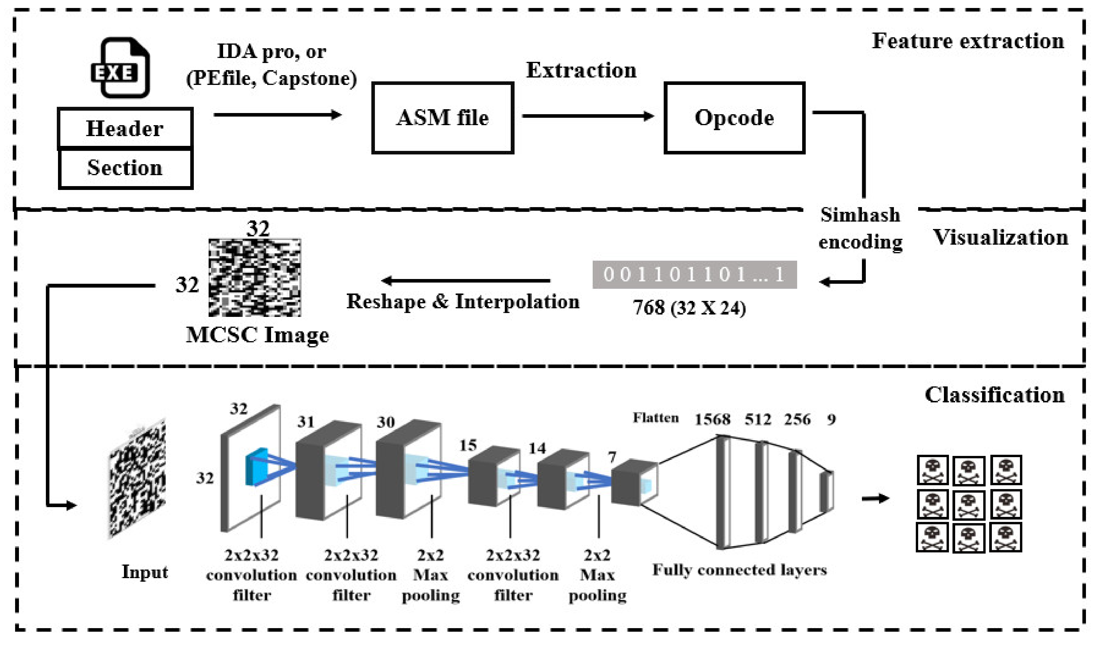
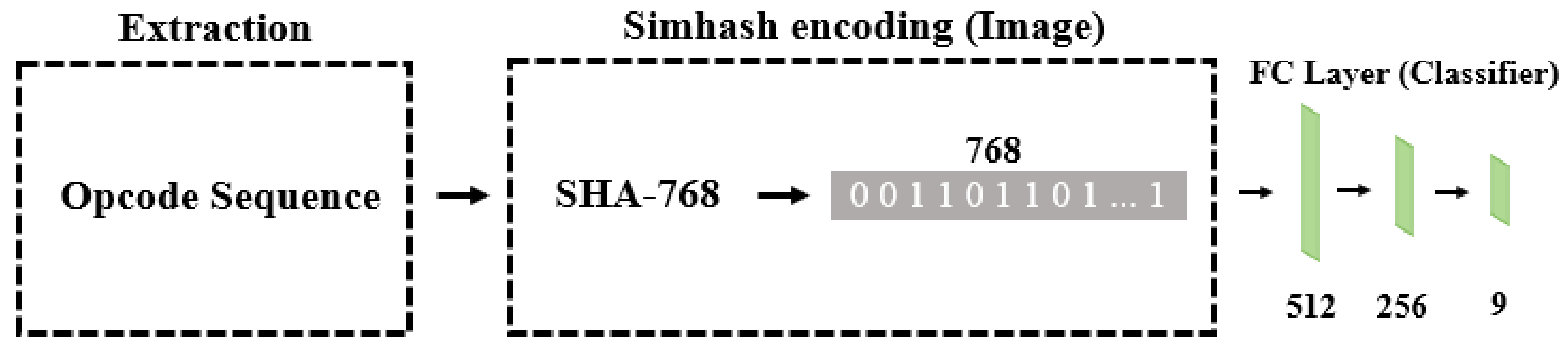
2.2. Simhash, N-Gram, MCSC Image and N-Gram MCSC

Simhash encoding is a local sensitive hash algorithm proposed by Charinikar (2002) and is mainly used for sequence similarity [7]. That is, similar words will have similar hash values.

The N-gram is a method that groups a given sentence or data as sequences of continuous combinations [8]. The size of the combination is defined according to N. When grouping data has N = 1, it is called a “unigram”, N = 2 is a “bigram” and N = 3 is a “trigram”. N-gram is not only used in natural language processing but also used effectively in malware detection. In [9], the author proposed multi-level big data mining using natural language processing (NLP) and machine learning (ML) techniques for detecting Ransom-ware attacks. N-gram and TF-IDF methods were used for making features and the result is dependent on different sizes of N with an accuracy of 98.59% obtained when N = 3.

The MCSC [4] is an algorithm for malware classification, which converts the executable file into an image and uses it as input data for the CNN network. We refer to this image an MCSC image. The overall procedure is shown in Figure 1.

The MCSC method has three phases: feature extraction, visualization, and classification. In feature extraction, all opcodes are extracted from the code section in the ASM file, which is made by a disassembler. In the visualization phase, Simhash encoding is undertaken using the opcode sequence. After encoding, the executable file is represented as a fixed length of binary code. Then, the binary code is reshaped into the pre-defined size and interpolated with bilinear interpolation, and the CNN classifier uses it for training.

The original MCSC used several techniques in the step of feature extraction and used SHA-768 simhash encoding, three convolution layers, 2 × 2 filters and 2 max-pooling layers in the classification step. We only used the same classifier of the MCSC method and interpolation techniques except major-block selection. The detailed parameters of the classifier of MCSC are shown in

Table 1. Detailed parameters for the classification in Figure 1.

Layer (Type)	Output Shape	Param #	Remarks
Conv2d	[−1, 32, 31, 31]	160
Tanh	[−1, 32, 31, 31]	0
Conv2d	[−1, 32, 30, 30]	4128
Tanh	[−1, 32, 30, 30]	0
MaxPool2d	[−1, 32, 15, 15]	0
Dropout2d	[−1, 32, 15, 15]	0
Conv2d	[−1, 32, 14, 14]	4128
Tanh	[−1, 32, 14, 14]	0
MaxPool2d	[−1, 32, 7, 7]	0
Dropout2d	[−1, 32, 7, 7]	0
Linear	[−1, 512]	803,328	|
Tanh	[−1, 512]	0	|
Linear	[−1, 256]	131,328	| FC classifier
Tanh	[−1, 256]	0	|
Linear	[−1, 9]	2313	|

because we are concerned with the performance of the classifier. There are three reasons why we used the SHA-768 in our model. First, it showed the best performance in previous MCSC research. Second, we want to compare its performance with our methods using a simple technique (PCA). Lastly, the SHA-768 is composed of SHA-512 and SHA-256, so we can anticipate the effect for the different scales of encoding.

The N-gram MCSC is a method that combines the N-gram and MCSC images [10]. It applies the N-gram method to the original opcode sequence (1-gram) to make an N-gram opcode sequence. We call this the N-gram MCSC image. The N-gram for the opcode sequence reinforces the semantic meaning of the chunked opcode sequence.

2.3. Principal Component Analysis (PCA)

PCA is a method for analyzing given data to find principal components through the distribution of the data, where the principal components are the direction vectors with sequentially high variances for the symmetrical covariance matrix of the data [11]. For example, suppose we have two or three-dimensional data. We can find a line that minimizes the distance from each point of the data to one straight line. This line is called as the first principle component of the data. Repeating the same system, we can find the second principle components which are the orthogonal vectors to each other, and each dimension is not correlated. We can obtain two principle components for two-dimensional data and three components for three-dimensional data. PCA can be used for many applications as it applies to many fields. The most popular applications of PCA are dimensionality reduction and exploratory data analysis [12]. Dimension reduction is used to reduce the dimensions of a given dataset to a certain size. For dimensionality reduction, we obtain all the principal components of the given data through PCA, and then the data is projected with the number of principal components that we desire. The number of components is the reduced dimension for the data. Avoiding the curse of dimensionality is one of the main advantages of dimension reduction. Exploratory data analysis is used to understand high-dimensional data using PCA. After finding the principle components, we can see the degree to which the first principal component can explain the data or how many components are needed to represent the dataset in the 90% variances. Also, we are able to visualize high-dimensional data in two or three dimensions.

3. Proposed Methods

3.1. Experimental Dataset

For the classification experiment, we used the Microsoft Challenge dataset [13], which has 9 classes and a total of 10,868 ASM files. With the exception of the files with no opcode after feature extraction, we used 10,736 of these files.

Table 2. The distribution of malware files.

Virus Name	Number of Files	TYPE
Ramnit	1532	Worm
Lollipop	2470	Adware
Kelihos_ver3	2937	Backdoor
Vundo	447	Trojan
Simda	39	Backdoor
Tracur	732	TrojanDownloader
Kelihos_ver1	387	Backdoor
Obfuscator.ACY	1179	Any kind of obfuscated malware
Gatak	1013	Backdoor

shows the distribution of malware files. It is highly imbalanced, with the main class being the Kelihos_ver3 virus with almost 3000 files, and a minor class being the Simda virus with 39 files [14].

In our dataset, there is Obfuscator.ACY category, which consists of any kind of obfuscated malware such as polymorphism or metamorphism to avoid detection systems. We cannot know what exact techniques are used. If the model can detect properly, we can say that the model is not vulnerable to countermeasures.

In our research, we experimented with Simhash (SHA-768) encoding according to the N-gram opcode sequence. The number of different opcode combinations is used to make N-gram Simhash encoding. This means that the size of the vocabulary dictionary is different. The vocabulary size of the N-gram is shown in

Table 3. The size of the vocabulary dictionary of N-gram.

N-Gram	The Size of the Vocabulary Dictionary of N-Gram
1-gram	231
2-gram	24,920
3-gram	24,916
4-gram	24,910

. In the case of the 1-gram, the size of the vocabulary dictionary is 231 words (it is the number of different opcodes).

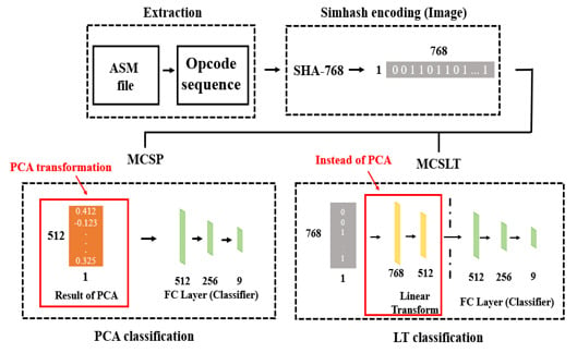
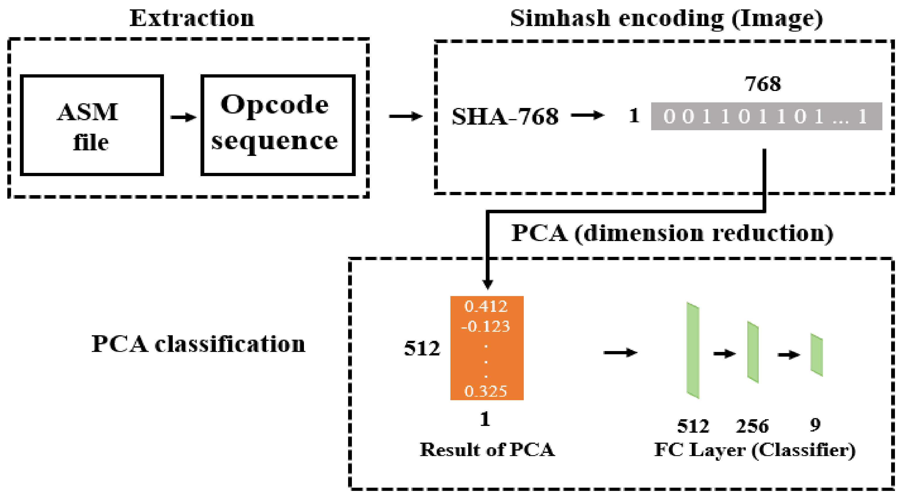
3.2. Method 1: Malware Classification Using Simhah Encoding and PCA (MCSP)

Before proposing our methods, we did a principal component analysis (PCA) analysis for Simhash encoding according to N-gram. We analyzed the variance explained by PCA of each Simhash encoding because different vocabulary size is mapped to the constant size (768). The results of the PCA analysis are shown in

Table 4. The number of principal component analysis (PCA) axis for explained variance against the total variance.

The Number of PCA Axis\N-Gram	1-Gram	2-Gram	3-Gram	4-Gram
The number of PCA axis for 95% explained variance	141	316	441	510
The number of PCA axis for 90% explained variance	53	162	278	358

and Figure 2.

In Figure 2, we visualized the cumulative variance according to the number of axes and marked the point for 95% explained variance of the N-gram. As shown in Table 4, the number of PCA axes for 95% explained variance of the 1-gram, 2-gram 3-gram and the 4-gram were 141, 316, 441 and 510, respectively. This indicated that we can reduce each of them by maintaining the 95 % variance of the 768-dimensional Simhash encoding. The number of PCA axes for 90% explained variance for the 1-gram, 2-gram 3-gram and the 4-gram were 53, 162, 278 and 358, respectively.

Based on the above results, we propose a malware classification method using Simhash encoding and PCA (MCSP). The overall procedure of the MCSP method is shown in Figure 3.

As shown in Figure 3, the MCSP method includes three steps: extraction, Simhash encoding, and PCA classification. In the extraction step, the opcodes sequence is extracted from an asm file. In the Simhash encoding step, the extracted opcode is encoded through Simhash (SHA-768). It is a multi-hash with SHA-512 and SHA-256 [15]. In the PCA classification step, the 768-dimensional Simhash encoding is reduced to 512-dimensional sequences by using the PCA algorithm. The reason for reducing Simhash encoding to 512 dimensions is to ensure that the total variance in the reduced data exceeds at least 95% variance. After that, the transformed sequence is used as an input feature for a fully connected (FC) classifier.

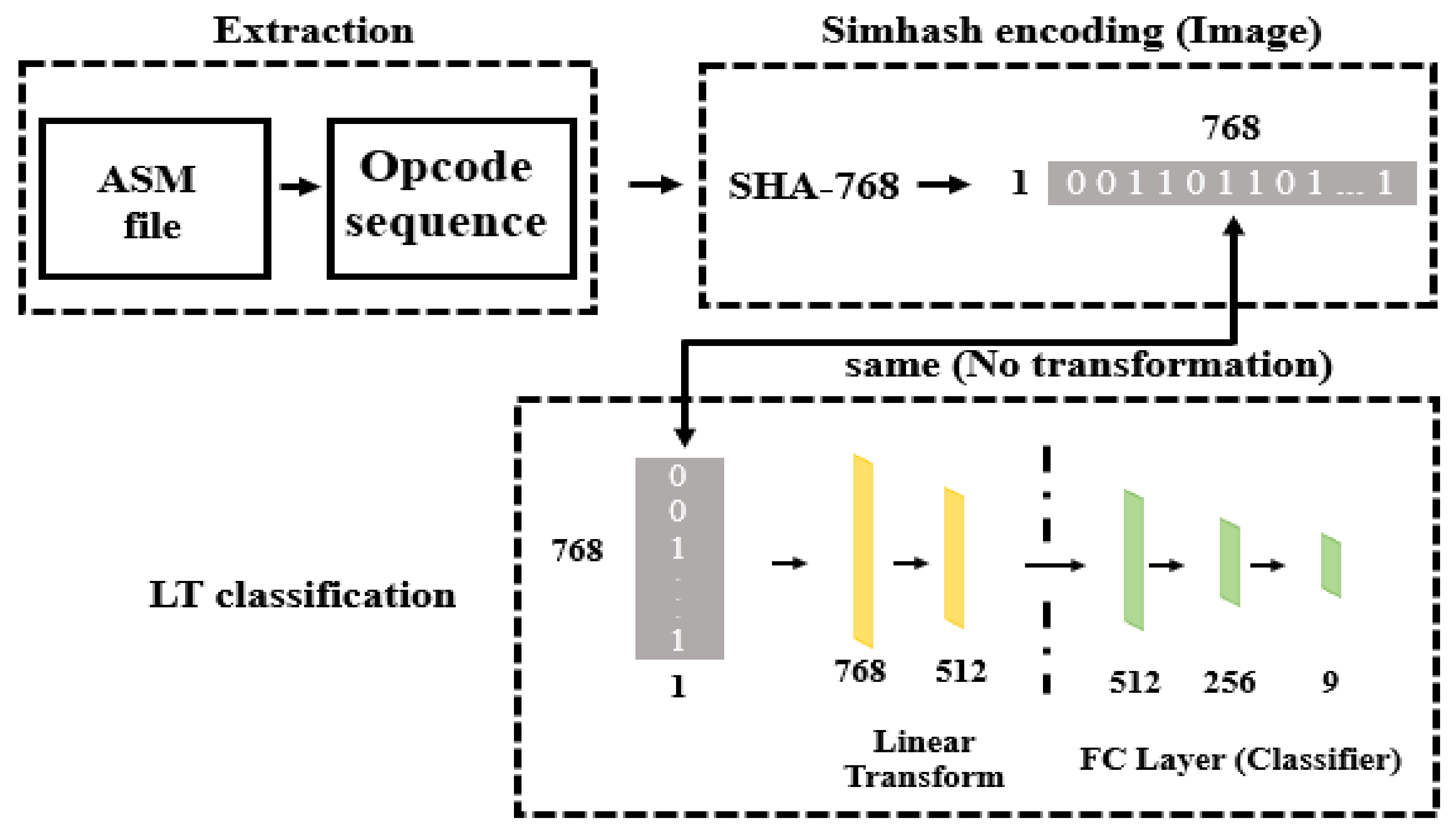
3.3. Method 2: Malware Classification Using Simhash Encoding and Linear Transformation Layer (MCSLT)

We propose another method for malware classification by using Simhash encoding and linear transform layer (MCSLT). It mimics the role of PCA by using a neural network with two layers, which are layers without an activation function. This transforming layer is known as the linear transform (LT) layer. The overall procedure of the MCSLT method is shown in Figure 4.

As can be seen in Figure 4, MCSLT works in three steps: extraction, Simhash encoding and LT classification. The first two steps are the same as the MCSP method. The Simhash encoding is used as the input for the LT layer. We think the first layer of LT reveals another coordinate system and the second layer of LT reduces the dimension. The intention is to let the model learn another coordinate system and reduce the dimension automatically. That is, LT layers are used to find a linear transformation similar to the PCA. The output of the LT layer is used as input features for the same FC layer as the MCSP method.

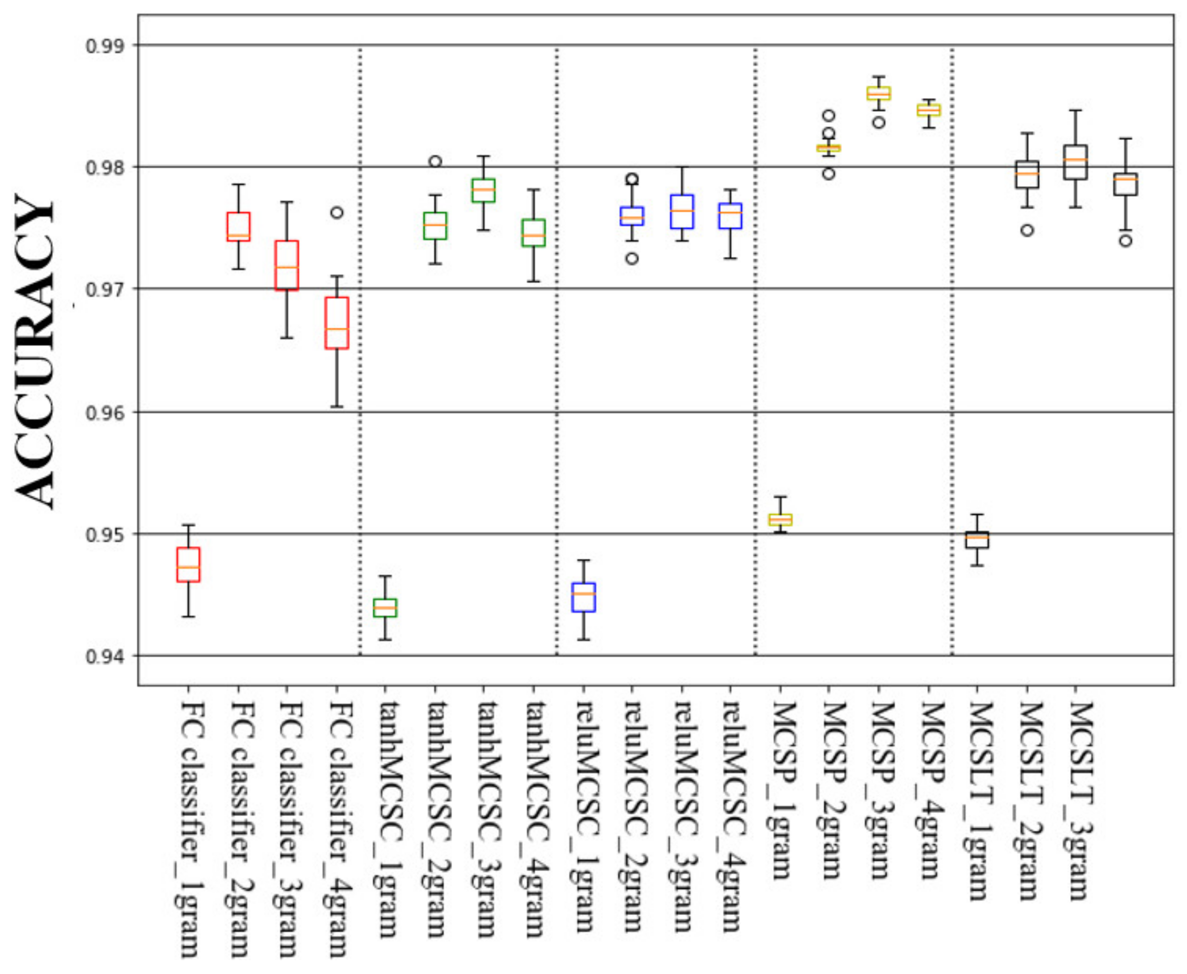
4. Experimental Results

We split the dataset into train and test datasets at a proportion of 8:2. Our hardware setting was Intel i7-7600 k, 64 GB memory and 2 Nvidia GeForce GTX 1080 Ti. We implemented the proposed methods with Python 3.6 and Pytorch 1.1.0 in the Jupyter Notebook environment, but we only used 1 gpu for these experiments.

The used Simhash encoding was a multi-hashing method: SHA-768. The SHA-768 consists of SHA-512 and SHA-256. After encoding the N-gram opcode sequence with the SHA-512 and the SHA-256, we combined the outputs. It is the binary sequence of 768 sizes.

To compare the performance of the proposed methods, we used the fully connected (FC) classifier. The overall procedure is shown in Figure 5.

The FC classifier is a simple classifier that uses Simhash encoding as an input feature for the FC layer. The FC layer consists of three dense layers that are 512, 256 and 9 sequentially. Each layer used the relu activation function. This is different to the original MCSC, which used the tanh function for activation, which is symmetric with respect to the original and its derivation is also symmetric. It is only used to measure the basic performance of Simhash encoding.

In the case of MCSC, it reshaped the Simhash encoding into a 32 × 24 image. Then, bi-linear interpolation was applied to make 32 × 32 square images. The interpolated image is used as input data for the CNN structure as shown in Figure 1. The neural network of MCSC consists of 3 convolutional layers using a 2 × 2 filter, tangent hyperbolic activation function and 2 max-pooling layers. This flattens the output of convolution layers and uses the fully connected layers.

In our experiment, we used the basic MCSC method. That is, we did not use any optimization technique in the original study. We also used the two versions of the MCSC method. The first is tanhMCSC, which uses the tanh activation function in the FC classifier and the second is the reluMCSC, which uses the relu activation function in the FC classifier.

The number of parameters for all of the compared methods, is shown in

Table 5. The total number of parameters according to the method.

Methods	FC Classifier	MCSC (tanh, relu)	MCSP	MCSLT
Model + Classifier layers	393,728 + 133,641	811,744 + 133,641	262,656 + 133,641	1246976 + 133,641
The total number of parameters	527,369	945,385	396,297	1,477,641

. The number of parameters for the classifier layers was calculated like this: 133,641 = (512 + 1) × 256 + (256 + 1) × 9. In the case of the FC classifier, we need additional parameters: that is 393,728 = (768 + 1) × 512. Therefore, the total number of parameters is 527,369 as shown in Table 5. The total number of MCSC, MCSP and MCSLT’ parameters are 945,385, 396,297 and 1,477,641, respectively. As a result, MCSP has the fewest parameters with a total of 396,297. However, MCSLT has 1.5 and 2.8 times more parameters than MCSC and FC classifier.

For hyper-parameters of the convolutional neural networks, we assumed the batch size was 64, the epoch was 500, the learning rate was 0.005 and the loss function was cross-entropy. For other models, we used the same batch size, epoch, loss function but the learning rate was 0.0001.

In order to compare the accuracy of the compared methods, we conducted the experiments 30 times for each method. Therefore, we can use a parametric test that is based on the normality of data. The accuracy boxplot for all of the compared methods is shown in Figure 6. In addition, the average and maximum accuracy for them is shown in

Table 6. The accuracy for all compared methods.

N-Gram\Methods		FC Classifier	tanhMCSC	reluMCSC	MCSP	MCSLT
1-gram	Mean	94.73	94.40	94.48	95.13	94.95
	Max	95.07	94.65	94.79	95.30	95.16
	Std	0.0020	0.0012	0.0017	0.0007	0.0011
2-gram	Mean	97.47	97.53	97.60	98.16	97.95
	Max	97.86	98.04	97.91	98.42	98.28
	Std	0.0018	0.0018	0.0014	0.0007	0.0017
3-gram	Mean	97.21	97.80	97.80	98.60	98.04
	Max	97.22	98.09	98.00	98.74	98.46
	Std	0.0031	0.0014	0.0016	0.0008	0.0019
4-gram	Mean	96.71	97.46	97.60	98.47	97.85
	Max	97.63	97.81	97.81	98.56	98.23
	Std	0.0033	0.0018	0.0014	0.0005	0.0020

.

According to Table 6, the FC classifier showed an average accuracy of 94.73%, 97.47%, 97.21% and 96.71% for 1-gram, 2-gram, 3-gram and 4-gram Simhash encoding, respectively. The tanhMCSC showed 94.40%, 97.53%, 97.80% and 97.46%, respectively. The reluMCSC showed 94.48%, 97.60%, 97.80% and 97.60%, respectively. The MCSP showed 95.13%, 98.16%, 98.60% and 98.47%, and he MCSLT showed 94.95%, 97.95%, 98.04% and 97.85%, respectively.

To examine whether the compared methods were statistically different, we calculated the analysis of variance (ANOVA), except for the FC classifier [16]. There was a significant difference (p value < 0.000) in the 1-gram and 2-gram Simhash encoding. In the post-hoc analysis, we used the Scheffe method with a 95% confidence level. As a result, we found three groups: tanhMCSC and reluMCSC, MCSLT, MCSP (in the order of their performance). There was a significant difference (p value < 0.000) for the 3-gram, which resulted in four groups being identified: reluMCSC, tanhMCSC, MCSLT, MCSP. There was a significant difference (p value < 0.000) for the 4-gram and four groups were identified: tanhMCSC, reluMCSC, MCSLT, MCSP.

With regard to accuracy, the MCSP method showed the best performance in spite using 2.4 times fewer parameters than the MCSC method and 3.7 times fewer parameters than MCSLT. In the case of MCSLT, it performed better than MCSCs for all N-grams. However, it used 1.6 times more parameters than the MCSC method.

We considered the problem of multi-class classification as several binary classification problems for each malware family. So, Precision, Recall and F1 score are common evaluation methods in classification problems. In multi-class classification, there are macro- and micro-average methods [17]. For example, suppose there are k classes, then, micro-averaging for Precision is calculated by the following formula.

$$PR{E}_{micro}=\frac{T{P}_1+\dots +T{P}_k}{T{P}_1+\dots +T{P}_k+F{P}_1+\dots +F{P}_k}$$

(1)

Macro-averaging for Precision is calculated by the following formula.

$$PR{E}_{macro}=\frac{PR{E}_1+\dots +PR{E}_k}{k}$$

(2)

The F1 score is calculated by the following formula.

$$\mathrm{F}1=\frac{2*Precision*Reall}{Precision+Reall}$$

(3)

In addition to accuracy, we measured the F1 score by using micro-averaging to evaluate the results for 30 run times. These are shown in Figure 7 and

Table 7. The Average F1 score using micro-averaging for all compared methods.

Methods		Ramnit	Lolli pop	Kelihos_ ver3	Vundo	Simda	Tracur	Kelihos_ ver1	Obfuscator. ACY	Gatak	Mean Score	Weighted Mean Score
1-gram	tanhMCSC	0.8193	0.9539	0.9999	0.9924	0.8524	0.9005	1	0.9159	0.9868	0.9357	0.9357
	reluMCSC	0.8417	0.9574	1	0.9924	0.8571	0.9084	1	0.9185	0.9859	0.9372	0.9694
	MCSP	0.8213	0.9699	1	0.9981	0.8571	0.918	1	0.9281	0.9948	0.9431	0.9696
	MCSLT	0.8146	0.9676	1	0.9936	0.8571	0.9126	1	0.9328	0.9924	0.9412	0.9685
2-gram	tanhMCSC	0.9556	0.9814	1	0.9962	0.8095	0.9267	1	0.9425	0.9826	0.9549	0.9549
	reluMCSC	0.9565	0.981	1	0.9951	0.8429	0.9336	1	0.9432	0.9832	0.9595	0.9779
	MCSP	0.963	0.9868	1	1	0.9333	0.9397	1	0.9555	0.9948	0.9748	0.9869
	MCSLT	0.9611	0.9834	1	0.9951	0.9476	0.932	0.9982	0.957	0.989	0.9737	0.9861
3-gram	tanhMCSC	0.9643	0.9767	0.9984	0.9788	0.7143	0.9724	0.9958	0.953	0.979	0.9481	0.9481
	reluMCSC	0.9608	0.9731	0.9988	0.9742	0.7333	0.9756	0.9970	0.9503	0.9782	0.9490	0.9719
	MCSP	0.9717	0.9897	1	1	0.9857	0.9795	0.9848	0.9592	0.9892	0.9844	0.9920
	MCSLT	0.9603	0.9842	0.9997	0.9898	0.7524	0.9749	0.9873	0.9536	0.9844	0.9541	0.9745
4-gram	tanhMCSC	0.9647	0.9782	0.9971	0.9697	0.7762	0.9231	0.9855	0.9583	0.9763	0.9477	0.9477
	reluMCSC	0.9592	0.9784	0.9988	0.9723	0.9000	0.9260	0.9891	0.9667	0.9763	0.963	0.9802
	MCSP	0.9779	0.9886	1	0.9886	0.6857	0.9797	0.9945	0.9595	0.9796	0.9505	0.9716
	MCSLT	0.9658	0.9844	0.998	0.9784	0.7429	0.9562	0.9909	0.9525	0.978	0.9497	0.9718

. We found the scores by using the function sklearn.merics.precision_ recall_fscore_support (…, …, average = ‘micro’). In this case, all metrics (Precision, Recall and F1 score) are the same. Therefore, we can also regard the results shown in Figure 7 and Table 7 as Precision or Recall.

For the 1-gram, the average micro F1 score of the tanhMCSC method were 81.93%, 95.39%, 99.99%, 99.24%, 85.24%, 90.05% 100%, 91.59% and 91.85% according to malware classes ranging from Ramnit through to Gatak. The mean F1 score of the tanhMCSC method was 93.57%. For the 1-gram Simhash encoding, the mean F1 score for the four compared methods were 93.57%, 93.72%, 94.31%, and 94.12%, respectively. In Table 7, we added the last column (shaded column), which shows the weighted macro F1 score. We found this score by using the function sklearn.merics.f1_score(…, …, average = ‘weighted’). We plotted the values of the last two columns in Table 7, the mean F1 score and the mean weighted F1 score, according to N-gram for the compared methods in Figure 8.

Our data is highly imbalanced, therefore, the weighted macro F1 score seemed to be the right metric to evaluate. Our MCSP and MCSLT showed better performance than the tanhMCSC method for all N-gram Simhash encoding. Our methods performed better than the reluMCSC method for the 1-gram, 2-gram and 3-gram. However, they showed a lesser performance for the 4-gram.

From the viewpoint of the weighted macro F1 score, MCSP showed the best performance with a value of 99.2% for the 3-gram. The MCSLT model showed the best performance with a value of 98.61% for the 2-gram, although, this value is less than the MCSP method. In the case of reluMCSC, the model showed the best performance with a value of 98.02% for the 4-gram.

5. Conclusions

In this paper, we proposed two malware classification methods known as the MCSP and MCSLT methods. The MCSP method classifies malware using Simhash encoding and PCA. It encoded the opcode sequences of ASM files to Simhash encoding and applied the PCA method to them. The MCSLT method applies the LT layer to Simhash encoding. The LT layer consists of two fully connected layers that mimic the linear transformation, which is similar to PCA.

The Microsoft Challenge public dataset was used to evaluate the performance of tanhMCSC, reluMCSC and the two proposed methods. With regard to the number of parameters for each model, our MCSP model is efficient because it has a simple structure compared to MCSCs that use CNN and it has fewer parameters than them. However, our MCSLT model has 1.6 times more parameters than MCSCs.

With regard to performance, we measured accuracy and F1 score using a micro-average and weighted macro-average. We conducted 30 experiments for Simhash encodings that are derived from the 1-gram, 2-gram, 3-gram and 4-gram opcode sequences. As a result of the experiments, the MCSP had the best maximum accuracy of 98.74% and an average accuracy of 98.58% for the 3-gram Simhash encoding. From the viewpoint of the F1 score using the weighted macro-average, the MCSP and MCSLT showed better performance than the tanhMCSC method for all N-gram Simhash encoding. Our proposed methods showed better performance than the reluMCSC method for the 1-gram, 2-gram and 3-gram. However, they showed less performance for the 4-gram.

The strengths of this paper are that we tackled a subject of current intensive research, the algorithms are very simple, and our methods have computational advantages compared to the existing methods. However, the main limitation of the study is that we did not use the label information for data.

References

1. Gandotra, E.; Bansal, D.; Sofat, S. Malware analysis and classification: A survey. J. Inf. Secur. 2014, 2014, 44440. [Google Scholar] [CrossRef] [Green Version]
2. Lu, R. Malware Detection with LSTM using Opcode Language. arXiv 2019, arXiv:1906.04593. [Google Scholar]
3. Nataraj, L.; Yegneswaran, V.; Porras, P.; Zhang, J. A comparative assessment of malware classification using binary texture analysis and dynamic analysis. Available online: http://www.csl.sri.com/users/vinod/papers/aisec17-nataraj.pdf (accessed on 2 March 2020).
4. Ni, S.; Qian, Q.; Zhang, R. Malware identification using visualization images and deep learning. Comput. Secur. 2018, 77, 871–885. [Google Scholar] [CrossRef]
5. Sun, G.; Qian, Q. Deep learning and visualization for identifying malware families. IEEE Trans. Dependable Secure Comput. 2018. [Google Scholar] [CrossRef]
6. Damodaran, A.; Di Troia, F.; Visaggio, C.A.; Austin, T.H.; Stamp, M. A comparison of static, dynamic, and hybrid analysis for malware detection. J. Comput. Virol. Hacking Tech. 2017, 13, 1–12. [Google Scholar] [CrossRef]
7. Charikar, M.S. Similarity estimation techniques from rounding algorithms. In Proceedings of the thiry-fourth annual ACM symposium on Theory of computing, Montreal, QC, Canada, 19–20 May 2020; pp. 380–388. [Google Scholar]
8. Witten, I.H.; Frank, E. Data mining: Practical machine learning tools and techniques with Java implementations. Acm Sigmod Rec. 2002, 31, 76–77. [Google Scholar] [CrossRef]
9. Poudyal, S.; Dasgupta, D.; Akhtar, Z.; Gupta, K. A multi-level ransomware detection framework using natural language processing and machine learning. In Proceedings of the 14th International Conference on Malicious and Unwanted Software” MALCON, Nantucket, MA, USA, 2–4 October 2019. [Google Scholar]
10. Lim, M.J.; Kwon, Y.M. Efficient algorithm for malware classification: N-gram MCSC. Int. J. Comput. Digit. Syst. 2020, 9, 179–185. [Google Scholar]
11. Wold, S.; Esbensen, K.; Geladi, P. Principal component analysis. Chemom. Intell. Lab. Syst. 1987, 2, 37–52. [Google Scholar] [CrossRef]
12. Zhang, T.; Yang, B. Big data dimension reduction using PCA. In Proceedings of the IEEE International Conference on Smart Cloud (SmartCloud), New York, NY, USA, 18–20 November 2016; pp. 152–157. [Google Scholar]
13. Ronen, R.; Radu, M.; Feuerstein, C.; Yom-Tov, E.; Ahmadi, M. Microsoft malware classification challenge. arXiv 2018, arXiv:1802.10135. [Google Scholar]
14. Krawczyk, B. Learning from imbalanced data: Open challenges and future directions. Prog. Artif. Intell. 2016, 5, 221–232. [Google Scholar] [CrossRef] [Green Version]
15. Dang, Q.H. Secure hash standard; (No. Federal Inf. Process. Stds.(NIST FIPS)-180-4); National Institute of Standards and Technology: Gaithersburg, MD, USA, 2015.
16. Miller, R.G., Jr. Beyond ANOVA: Basics of applied statistics; CRC Press: Boca Raton, FL, USA, 1997. [Google Scholar]
17. Van Asch, V. Macro-and micro-averaged evaluation measures. Available online: https://pdfs.semanticscholar.org/1d10/6a2730801b6210a67f7622e4d192bb309303.pdf (accessed on 2 February 2020).
Figure 1. The overall procedure of malware classification using Simhash and CNN (MCSC) algorithm.
Symmetry 12 00830 g001
Figure 2. The graph of cumulative variances according to the number of axes.
Symmetry 12 00830 g002
Figure 3. The overall procedure of the malware classification using Simhash and PCA (MCSP) method.
Symmetry 12 00830 g003
Figure 4. The overall procedure of the malware classification using Simhash and linear transform (MCSLT) method.
Symmetry 12 00830 g004
Figure 5. The overall procedure of the fully connected (FC) classifier.
Symmetry 12 00830 g005
Figure 6. The accuracy boxplot of all compared methods.
Symmetry 12 00830 g006
Figure 7. Average F1 score using micro-averaging for all compared methods.
Symmetry 12 00830 g007
Figure 8. Mean (Precision, Recall, F1) score (a) and mean weighted macro score (b) for compared methods.
Symmetry 12 00830 g008