Abstract
Distributed systematic grid-connected inverter practice needs to improve insulated gate bipolar transistor (IGBT) stability to ensure the safe operation. This study is to ensure the safety and reliability operation of the IGBT module in symmetry to meet the reliable and stable distributed systematic grid-connected inverter practice and the junction temperature is a parameter to assess its operating state. It is difficult to accurately acquire the IGBT junction temperature to be solved by a single method of combining the test and the modeling. The saturation voltage drop or collector current and module junction temperature data under different power cycles are measured by the power cycle test and the single pulse test. The improved chicken swarm optimization increases the chickens diversity and self-learning ability. The prediction model of the improved chicken swarm optimization-support vector machine is proposed to forecast the module junction temperature. The result showed to compare with the particle swarm optimization-support vector machine model and chicken swarm optimization-support vector machine model and showed the coincidence degree between the proposed model prediction value and the true value is higher. The mean absolute error ratio indicates the proposed model has a smaller error and a better prediction performance. The proposed model has a positive impact on improving the distributed systematic grid-connected inverter industrial development and promotes the new energy usage.
1. Introduction
The distributed photovoltaic (PV) grid-connected inverter performance directly affects the distributed PV power generation development. The PV industry has experienced the most growth in the last decades due to its desirable characteristics of high economic efficiency, sustainability, and low pollution [1]. As new energy technology development has promoted the exploitation and utilization of new energy. The new energy technology has a positive impact on promoting sustainable economic development and protecting the environment. With the development of society, traditional fossil energy sources not only cause serious environmental pollution, but also are increasingly exhausted, which makes scientists strive to study new energy and seek the path of sustainable development [2,3,4]. In practices, promoting the energy transformation and achieving sustainable development are important issues for the development of mankind [5,6]. The primary goal of sustainable development is to achieve rational use of new energy and improves the energy utilization.
In the literature, Preda et al. [7] addressed numerical approach for off-grid systems to provide an accurate forecast of the PV output is important. Malik et al. [8] proposed a new boost converter based on the dynamic modeling method and compared with the conventional secondary converter in various parameters to obtain high voltage gain without operating at the maximum duty cycle. The adaptability of the Z-source inverter is limited due to the discontinuity of the source current. Anwar et al. [9] presented a new Z inverter to provide three-stage AC output in a single stage and boost the DC voltage to the required level. Wang et al. [10] argued various variables based modeling for the distributed PV grid-connected system and proposed the model of the PV power plant consists DC optimizers in a heavy computation burden during the simulation. New high-efficiency corresponding distributed control strategies of power converters have been presented to ensure optimal energy harvest from the PV array in different shading scenarios [11]. Beilski et al. [12] presented the modification of proportional-integral controller for tracking of the grid-connected photovoltaic micro inverter output and the micro inverter output current sinus shape distortions decrease when the ordinary PI controller is used. The development of distributed systematic grid-connected inverter practice has positive significance for the development of renewable energy [13,14]. This study proposes to fulfill the existed gaps from prior studies.
Especially, the IGBT module in symmetry is a vital component of the power system of distributed systematic grid-connected inverter practice. The insulated gate bipolar transistor (IGBT) is a relatively fragile device. If IGBT fails, the whole system stops working [15,16]. The operational IGBT module reliability and stability is improved by technical a method, which is of strategic significance for further promoting the new energy development [17]. The switching loss of the IGBT generates a large amount of heat, which causes a large temperature rise and excessive temperature rise affects the reliable operation.
For instance, Li et al. [18] used support vector machine (SVM) to forecast the switching loss. The SVM parameters are optimized by the chicken swarm optimization (CSO) algorithm. The switching losses are accurately predicted by SVM model. Chen et al. [19] proposed a method to diagnose bond line peeling. In this method, the on state voltage and the voltage on the emitter terminal are analyzed to judge. Moosavi et al. [14] analyzed the IGBT open circuit fault. The current waveform is extracted by using the wavelet transform. A variety of algorithms are used to classify faults. For instance, Yu et al. [20] proposed a new type of IGBT open circuit fault diagnosis algorithm to improve the diagnosis speed. The average value of the difference between the actual three-phase current and the reference three-phase current value in one electrical cycle is used as the judgment amount. In lieu of this, this study is to improve the reliability and recognition speed of fault diagnosis.
The literature are based on the physical model to analyze the power loss, junction temperature, IGBT switching loss and other characteristics. The modeling process of physical model is more complex, and the cost is higher. This study adopts SVM model compared with machine learning model. The SVM model has fewer parameters and stronger generalization ability compared with other machine learning models. The objectives of this study are as follows:
- To improve the search performance of the intelligent optimizer, so as to achieve the best convergence;
- To achieve the best SVM performance model using the SVM parameters optimized by an intelligent optimizer;
- To address the IGBT junction temperature prediction accuracy by optimizing the model parameters.
This study contributes to: (1) this study proposed an enhanced intelligent optimizer, which has strong convergence ability; (2) the improved chicken swarm optimization-support vector machine (ICSO-SVM) model is proposed to predict the IGBT junction temperature in this study, and better results were obtained; and (3) the model proposed has a positive impact on promoting the development of the distributed systematic grid-connected inverter industry and the use of new energy.
The rest of the study is structured as follows. Section 2 analyzes prediction methods of the junction temperature. Section 3 includes the materials and methods of this study. Section 4 mainly introduces the establishment process of junction temperature prediction model. The IGBT junction temperature is predicted in Section 5 by using the method proposed in this study. Section 6 provides the theoretical and engineering implications. Section 7 gives the important conclusions of this study.
2. Literature Review
This section includes the relevant literature of forecasting methods of junction temperature and the proposed method.
2.1. The Forecasting Methods of Junction Temperature
In practices, the IGBT module is aging with the accumulation of working hours, and its reliability is gradually decreasing. The IGBT failure in the power converters is affected by the thermal cycle [21]. The junction temperature is an important parameter to reflect the IGBT module in symmetry operating state. The higher the IGBT junction temperature is, the lower the operational safety is [22,23]. Fabis et al. [24] showed that the junction temperature rises by 10 °C, the failure rate is double. The IGBT junction temperature changes with time. Liu et al. [25] proposed a multi-time scale IGBT junction temperature prediction model based on the characteristics. The model is based on the semiconductor physics model and the short-term transient microsecond prediction model. Chen et al. [26] proposed an electro-thermal-based junction temperature estimation model. This model uses interpolation to calculate the power loss of the converter. At the same time, the RC network model is established to estimate the junction temperature considering thermal coupling effects and dissipation boundary conditions. Bazzo et al. [27] proposed a measurement method by mounting a fiber-optic sensor on the IGBT chip structure. The junction temperature is monitored online by building a thermal model. Then the results are used to simulate the heat generated by the IGBT switch process. However, the process of installing the sensor is complicated, which is difficult to improve the measurement accuracy. It is not suitable to measure the junction temperature directly by using the instrument and to find a suitable junction temperature prediction method.
The IGBT junction temperature prediction model is divided into two categories. One is based on the electro-thermal coupling model and the other is based on the intelligent algorithm. The former is a common method. Furthermore, its process includes the establishment of the IGBT power loss model and the establishment of the Foster or Cauer thermal network model. Liu et al. [28] investigated the effects of aging of different electro-thermal parameters on junction temperature and case temperature. The electro-thermal parameters are inputs to the established electro-thermal coupling model to obtain the junction temperature and the shell temperature under different aging conditions. Tang et al. [29] proposed an improved IGBT parallel thermal impedance model. Based on the loss model and thermal impedance model, the parallel IGBT electro-thermal model is established. The model is used to compare the effects of different module installation distances on transient junction temperature. Xie et al. [30] analyzed the mean power loss and thermal model. Then a suitable model is built to predict the junction temperature in high frequency applications. Li et al. [31] found that the IGBT aging seriously affected the accuracy of calculation results. The electro-thermal coupling model has certain limitations.
Aforementioned, the electro-thermal coupling model is used to calculate the IGBT junction temperature. However, there are few studies on the junction temperature by using the intelligent algorithm. In general, the junction temperature prediction model based on the intelligent algorithm is built by obtaining the values of junction temperature and the electro-thermal parameters. This method mainly establishes the mathematical model of the electro-thermal parameters and the junction temperature. Following this, the IGBT junction temperature is predicted by using the mathematical model. The primary work of establishing the junction temperature prediction model based on the intelligent algorithm is the junction temperature measurement. The general method of junction temperature measurement is the thermistor parameters method, which is to find the corresponding relationship between the thermistor parameters and the junction temperature. Eleffendi et al. [32] combined the IGBT electro-thermal parameters (thermal impedance or saturation voltage drop) with the method of Kalman filtering to predict the junction temperature. But this method does not consider the influence of IGBT aging on the junction temperature.
2.2. The Proposed Method
Cortes and Vapnik, [33] proposed the support vector machine (SVM). SVM is suitable for small sample and nonlinearity occasions. Gao et al. [34] proposed a model to predict the life of lithium batteries. This method uses particle swarm (PSO) to optimize the multi-core SVM. The results show that the model not only has a better prediction accuracy but also reduces the computational complexity. Wang et al. [35] used the SVM to analyze high-throughput experimental data. Based on the response surface generated by the SVM model, the correlation between experimental factors and the diversity of silanol group is determined. Meng et al [36] proposed the chicken swarm optimization (CSO) algorithm. The CSO algorithm mimics the hierarchical order and the behaviors of chicken swarm. The optimization performance and robustness of the CSO algorithm are better compared with other traditional algorithms. Zouache et al. [37] solved multi-objective optimization problems by CSO algorithm and the CSO algorithm was improved. In the ICSO algorithm, the aggregate function is used to define social ranks and the behavior of chickens in the search for food is simulated in the target search space.
Based on the IGBT test data, this study uses the improved chicken swarm optimization (ICSO) algorithm to optimize the parameters of the SVM. The specific improvement points of the CSO algorithm are as follows: (1) The self-learning ability of roosters, hens and chicks is improved by using a dynamic inertia reduction strategy. (2) In the later stages of the CSO algorithm, the variation of the roosters is changed from Gaussian variation to Cauchy variation, which increases the diversity of the group. (3) The roosters and the chicks learn from the global optimal individual. Further, the junction temperature prediction model is established. The IGBT aging state, saturation voltage drop and current are taken as input parameters and the junction temperature is taken as output parameter.
3. Method
The power cycle test platform and the single pulse test platform were built. Further, the saturation voltage drop, current and junction temperature were obtained under different power cycles.
3.1. Power Cycle Test
The study and test of IGBT began in 1994 [38,39]. So far, its failure modes mainly include the following aspects: (1) The bounding wire of IGBT falls off or fractures [40,41]. (2) The solder layer of IGBT is layered or disconnected [42,43]. (3) The IGBT silicon oxide is degraded [44]. There are many failure standards of IGBT. The common failure standard which is that the junction-to-case thermal resistance of IGBT increases by 20% compared with the initial value is selected in this study. When the junction-to-case thermal resistance reaches the failure standard, the power cycle test is ended.
The power cycle test is performed on the IGBT of the type MMG75S120B (MACMIC, Changzhou, Jiangsu, China), and the power cycle test circuit of IGBT is shown in Figure 1. The method of power cycle test is to repeatedly turn on and off the IGBT module in symmetry at a certain frequency. The power loss in the on-state makes the module temperature rise to a certain temperature (125 °C is selected in this study). The off-state module radiates heat to the ambient temperature of 25 °C through the radiator. The specific steps are as follows.
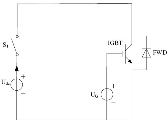
Figure 1.
The power cycle test circuit of insulated gate bipolar transistor (IGBT).
Figure 1 presents that the circuit is controlled to turn on or off S1. UG is 15 V, which ensures that the IGBT is always triggered. FWD is the freewheeling diode. The process of the power cycle test is presented according to IEC 60747-9:2007.
- The S1 is closed. The output current of Udc is set to 70 A. Further, the IGBT is driven. In this process, the junction temperature and case temperature of IGBT gradually rise from the ambient temperature.
- When the case temperature detected by the K-type thermocouple reaches 125 °C, the S1 is turned off. The junction temperature and the case temperature are rapidly decreased until the temperature drops to 25 °C. So far, a power cycle is completed.
- Step (2) and step (3) are repeated until the IGBT reaches the failure standard. The junction-to-case thermal resistance of IGBT increases by 20% compared with the initial value.
During the power cycle test, it is necessary to measure the junction-to-case thermal resistance to determine whether to stop the test. The transient thermal impedance of the IGBT is measured according to the YB-6911 thermal resistance test system of Xi’an Yibang Electronic Technology Co., Ltd. (Xi’an, Shaanxi, China). The test system meets the JEDEC51-1 standard, and the test current is 20 A with an accuracy of ±10 mA. The transient thermal impedances of the IGBT under different power cycles are shown in Figure 2.
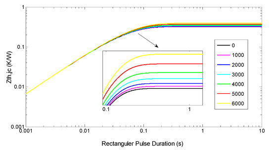
Figure 2.
The transient thermal impedances of the IGBT under different power cycles.
Figure 2 presented the transient state junction-to-case thermal impedance of the IGBT gradually increases with time and eventually tends to be stable. During the test, the steady state junction-to-case thermal impedance of the IGBT gradually increases with the increase of the number of power cycles. The increased magnitude is larger and larger.
The equation for calculating the junction-to-case thermal impedance is as follows.
where is the junction-to-case thermal impedance, is the thermal resistance, is the thermal capacitance, is the order of the thermal network, is the time.
Equation (1) showed when tends to infinity, the value of the junction-to-case thermal resistance is equals to the value of the transient state thermal impedance. Therefore, the junction-to-case thermal resistance reflects the aging state of the IGBT module in symmetry. According to the data of junction-to-case thermal resistance under different power cycles, the raw data curve is the black curve in Figure 3. In order to find the specific relationship between the IGBT junction-to-case thermal resistance and the number of power cycles. The black curve is fitted by the polynomial fitting method and the fitting curve is shown in Figure 3.
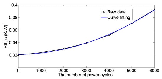
Figure 3.
The relationship between the IGBT junction-to-case thermal resistance and the number of power cycles.
The two curves are compared in Figure 3. It is found that the curve fitting has a high fitting degree. The polynomial fitting model obtained in Figure 3 is as follows:
where is the number of power cycles, is the junction-to-case thermal resistance.
The IGBT module coefficients in Equation (2) are presented as , and . The root mean square error after fitting is 0.0009.
In summary, the number of power cycles (the aging state) is obtained by measuring the IGBT junction-to-case thermal resistance.
3.2. Single Pulse Test
During the power cycle test, the test is suspended once every 1000 power cycles. The single pulse test is performed on the IGBT module in symmetry to measure the saturation voltage drop, current and junction temperature of the IGBT in the current power cycle. The single pulse test circuit of IGBT is shown in Figure 4.
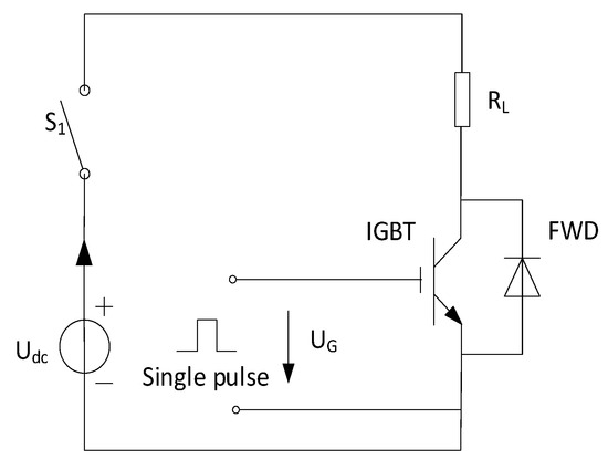
Figure 4.
The single pulse test circuit of IGBT.
The test points are selected as follows. For the temperature setting, the temperature of incubator increases from 25 °C to 125 °C, and 10 °C is increased each time. For the current setting, the current generated by Udc increases from 25 A to 150 A, and 5 A is increased each time. The pulse width under test should be small enough to avoid a rise in junction temperature caused by large current. RL is the power resistance. The specific test process is as follows:
- The IGBT is placed in the incubator and the temperature of the incubator is adjusted point by point according to the above description.
- When the IGBT reaches thermal equilibrium, the case temperature and junction temperature are equal to the incubator temperature. Then the selected current point is set in turn. The IGBT is triggered by single pulse. The saturation voltage drop value is measured by using voltage probe.
3.3. Test Results
The increments of the IGBT junction-to-case thermal resistance are more than 20% compared with the initial value after the power cycle 6000 times. Then the tests are stopped. The saturation voltage drop Vce, current Ic and junction temperature Tj of the IGBT under different power cycles are obtained. The test data at currents 65 A, 70 A, 75 A and 80 A are selected as modeling data. Based on the modelling data, the relationships between current, junction temperature and saturation voltage drop under different power cycles is obtained, which are shown in Figure 5.
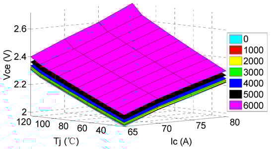
Figure 5.
The relationships between Ic, Tj and Vce under different power cycles.
Figure 5 presented that the numbers 0, 1000, 2000, 3000, 4000, 5000 and 6000 are the times of power cycles. With the aging of the IGBT, a three-dimensional surface composed of Ic, Tj and Vce is moved up overall, which indicates that Tj of the IGBT is closely related to the power cycles. The influence of the number of power cycles on the Tj should be fully considered in the process of establishing the IGBT junction temperature prediction mode.
4. The Establishment Process of Junction Temperature Prediction Model
The prediction model is based on the SVM. The SVM parameters are optimized by ICSO algorithm. The ICSO-SVM model is established.
4.1. Support Vector Machine
Vapnik et al. [45] proposed the SVM. SVM is a kind of machine learning method based on statistical learning theory. SVM enhances its generalization ability through the principle of structural risk minimization. Thereby, the goal of minimizing the empirical risk and confidence range is achieved. SVM is commonly used to solve problems of small samples, nonlinearities, and fault classification [46,47].
SVM is widely used in the field of regression prediction based on the advantages of strong generalization ability. Suppose a sample set is , is the input value of ith training sample, is the output value of ith training sample and represents the feature vector. In the feature space, the model corresponding to the division hyperplane is expressed as follows [48]:
where is an offset, is a weight vector, is the mapping function.
The optimal classification hyperplane problem is transformed into the following solving model.
The regression problem becomes a problem of minimizing the structural risk objective function according to the principle of structural risk minimization. The specific objective function and constraints are expressed as follows:
where is the penalty parameter, is the relaxation factor, and is insensitive loss function.
The Lagrange function is used to transform the inequality constrained optimization problem, and then the optimal value is solved by differentiation. The Lagrange multipliers are introduced to construct a Lagrange function. Equation (5) is transformed into the following constraint problem:
Finally, the nonlinear regression function is as follows:
where is the kernel function. The common kernel functions are as follows:
(1) Polynomial kernel function:
(2) Linear kernel function:
(3) Radial basis kernel function (RBF kernel function):
The RBF kernel function has the following advantages. (1) RBF kernel function achieves nonlinear mapping; (2) RBF kernel function has fewer parameters to reduce the complexity of the model; and the (3) RBF kernel function has less numerical calculation. The RBF kernel function is chosen owing to its advantages.
4.2. The CSO Algorithm and the ICSO Algorithm
4.2.1. The CSO Algorithm
Meng et al. [36] proposed the CSO algorithm to solve optimization problem by imitating the foraging characteristics and the hierarchy of chicken swarm. The chicken swarm usually consists of roosters, hens and chicks. The whole chicken swarm is divided into several small subgroups, each of which is composed of a rooster, several hens and chicks. At the same time, there is a competitive relationship between the small populations. There is a hierarchy subgroup, and each chicken has its own movement rule. In a subgroup, the rooster is in the leading position; the chicks follow the hens around the rooster. Compared with particle swarm optimization algorithm, genetic algorithm and differential evolution algorithm, the robustness and optimization ability of the CSO algorithm are stronger. The convergence speed is faster and the precision is higher [49,50]. The hierarchy of chicken swarm is formulated as follows:
- The whole chicken swarm is divided into several subgroups, and each subgroup consists of a rooster, multiple hens and chicks.
- The rooster is the leader in each population, and each population has only one rooster which has the strongest search ability. The search ability of hen is worse than of cock. The chicks follow the hens to search food, and the chicks have the worst search ability.
- The mother-child relationship between the hens and the chicks is updated at each iteration.
There is a total of chickens in the whole chicken swarm. The number of roosters is . The number of hens is . The number of chicks is .
The trajectory of rooster is expressed as follows:
where indicates the position of ith individual in the jth dimension after t + 1 iterations. represents a Gaussian distribution with a mean value of 0 and a standard deviation of . is determined by the individual fitness, which is expressed as follows.
where , is the fitness of the ith individual in the populations, indicates the fitness of a random individual in other populations, is infinitesimal to avoid the denominator is 0.
The trajectory of hen is expressed as follows.
where is a random number with uniformly distributed by [0, 1]. indicates the position of the rooster in the population where the hens are located. indicates the position of a random individual in the population. indicates the fitness value of the rooster. indicates the fitness value of a random individual.
The position of the chick in the population is determined by the hens which have a mother–child relationship with the chicks. The position update equation of the chick is expressed as follows:
where indicates the following coefficient of ith chick to the hen, and its value is a random number between [0, 2]. indicates the position of the hen which has the mother-child relationship with the ith chick.
4.2.2. The ICSO Algorithm
The CSO algorithm is a novel algorithm with a better optimization performance, but the CSO algorithm is easy to fall into local optimum under certain conditions. To avoid the phenomenon and enhance the global optimization ability of CSO algorithm, the CSO algorithm is improved. The roosters are the leaders in the whole chicken swarm. If the self-learning ability of roosters is reduced, the optimization process of the CSO algorithm is seriously affected. In order to solve the above problems, the learning rules of rooster are re-established. The details are as follows:
- (1)
- The weight is adjusted by the dynamic inertia learning strategy. The reduction strategy is adopted for improving the convergence speed of algorithm.
- (2)
- To solve the problem that the populations gradually decrease in the iterative process, in the later stage of algorithm, the Gaussian mutation process is changed to the Cauchy mutation process, which improves the diversity of the population.
- (3)
- The part of learning from the global optimal individual is added.
The improved update position equation of the rooster is as follows:
where represents the Cauchy distribution. is the optimal individual position. M is the maximum number of iterations. The equation of the dynamic inertia weight is as follows:
The size of the weight affects the search ability of the algorithm. The large weight is better for global search, and the small weight is better for local search. According to Equation (18), the is reduced from 0.9 to 0.4.
The hens account for the largest number of groups. The chicks look for food around the hens. The hens have great influence on the optimization effect. is added to the position update equation of the hen. The specific implementation is as follows:
Equation (19) showed that hens realize self-learning according to dynamic inertia weight, which improves the flexibility of the hen.
The chick has the worst-learning ability in the whole chicken swarm and learns from the hen. If the hen is fallen in local optimum, the search ability of the chick is significantly reduced. Therefore, this study improves the position of the chick from three aspects:
- is added to the position update equation to enhance the self-learning ability of the chick.
- The part of learning from the global optimal individual is added.
- When the fitness value of the chick remains unchanged during multiple iterations, the position of the chick is reset to avoid premature convergence.
- The improved position update equation of the chick is as follows.where is the fitness value of the optimal individual.
4.3. The Establishment Process of ICSO-SVM Model
The random parameters (kernel parameter and penalty parameters) of the SVM model have great influence on the prediction of junction temperature. The ICSO algorithm is used to optimize penalty parameter and the RBF kernel parameter. The number of power cycles, Ic and Vce are used as input variables of the proposed model to forecast the Tj.
The specific implementation steps are as follows:
- (1)
- The training samples and test samples are selected and normalized.
- (2)
- The number of roosters, hens and chicks in the chicken swarm and the number of iterations are set.
- (3)
- The population is initialized and the fitness value of the individual is calculated. The chicken swarm is divided into population. The hens randomly enter different populations.
- (4)
- The position of the rooster, hen and chick is updated according to Equations (17), (19) and (20). The fitness values of the swarm are calculated.
- (5)
- If the current individual fitness is better after the position update, the individual position is updated. Otherwise, the original individual position is maintained.
- (6)
- Determine whether the fitness of the chick remains unchanged after multiple iterations (five times). If the fitness value remains unchanged. The position of the chick is reset.
- (7)
- The fitness of each individual is calculated after each position update.
- (8)
- Determine whether the maximum number of iterations reaches. If it is satisfied, the optimal parameters are output. Otherwise, the parameters continue to be optimized.
- (9)
- The optimal parameters are input into the ICSO-SVM model. The junction temperature is forecasted by the ICSO-SVM model. The predictive results are inverse normalized.
The modeling process of prediction model of junction temperature is showed in Figure 6.
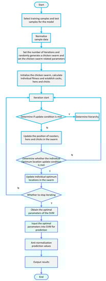
Figure 6.
The modeling process of the improved chicken swarm optimization-support vector machine (ICSO-SVM) junction temperature prediction model.
5. Results
In order to verify the prediction accuracy of the ICSO-SVM model for the distributed grid-connected system, the prediction values of the PSO-SVM model, CSO-SVM model and ICSO-SVM model are compared. Based on the data obtained by the power cycle test and the single pulse test, the 308 sets data at currents of 65 A, 70 A, 75 A and 80 A are selected to train and test CSO-SVM model and ICSO-SVM model. In the process of selecting data, 260 sets of data are randomly selected as the training samples, and the remaining 48 sets of data are test samples. The number of power cycles, Ic and Vce are selected as the input parameters. Tj is selected as the output parameter. The initial setting parameters of the PSO-SVM model are shown in Table 1. The initial setting parameters of the CSO-SVM model and the ICSO-SVM model are shown in Table 2.

Table 1.
Initial setting parameters of particle swarm optimization (PSO)-SVM model.
Table 2.
Initial setting parameters of chicken swarm optimization (CSO)-SVM model and ICSO-SVM model.
In order to verify the validity and practicability of the ICSO-SVM model, the ICSO-SVM model is used to predict the value of Tj. The absolute error (AE), relative error (RE), mean relative error (MRE), root mean square error (RMSE) and mean absolute error (MAE) are used to evaluate the test results of the ICSO-SVM model.
In the process of establishing PSO-SVM, CSO-SVM and ICSO-SVM models, the iterative curves obtained by randomly calculating three times are shown in Figure 7.
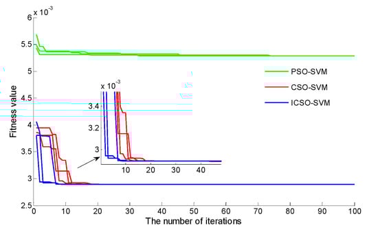
Figure 7.
The iterative curves of models.
Figure 7 presented the iterative curve of the PSO-SVM model tends to be stable when the number of iterations is 76, and the fitness value is 5.29 × 10⁻³. The iterative curve of the CSO-SVM model tends to be stable when the number of iterations is 18, and the fitness value is 2.89 × 10⁻³. The iterative curve of the ICSO-SVM model is basically stable when the number of iterations is 7, and the fitness is 2.89 × 10⁻³. The iterative stability times and fitness value of the ICSO-SVM model are better than other models.
The prediction curves of Tj and predictive errors of the PSO-SVM, CSO-SVM and ICSO-SVM models are presented in Figure 8, Figure 9 and Figure 10.
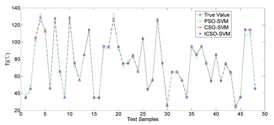
Figure 8.
IGBT junction temperature prediction curve.
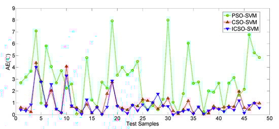
Figure 9.
The absolute error of IGBT junction temperature prediction curve.
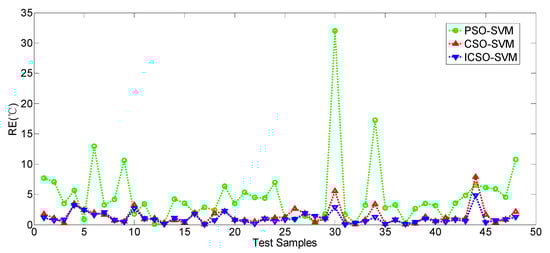
Figure 10.
The relative error of IGBT junction temperature prediction curve.
Figure 8, Figure 9 and Figure 10 showed that the prediction effect of PSO-SVM model is poor. The relative error and absolute error of PSO-SVM model are large. The prediction effect of CSO-SVM model is better than PSO-SVM model, and the relative error and absolute error are smaller than that. The prediction effect of ICSO-SVM model is the best. The relative error and absolute error of ICSO-SVM model are the smallest. In order to more intuitively compare the prediction effects of three models, the comparison chart and the comparison table of MAE, MRE and RMSE are established, as shown in Figure 11 and Table 3.
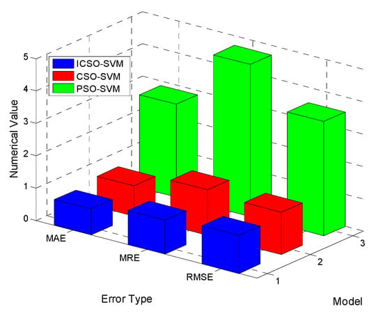
Figure 11.
The prediction errors of various models.
Table 3.
Comparison of prediction errors.
Figure 11 and Table 3 indicated the error of the PSO-SVM model is the largest, the error of the ICSO-SVM model is the smallest. The MAE ratio of PSO-SVM, CSO-SVM and ICSO-SVM model is: 2.8695:0.9316:0.7989 = 1:0.3247:0.2784, and the ratio of MRE is 4.7003:1.4068:1.0560 = 1:0.2993:0.2247. The ratio of RMSE is 3.5308:1.3121:1.1836 = 1:0.3716:0.3352.
6. Implications
The distributed grid-connected system is important for IGBT junction temperature to be calculated by the electro-thermal coupling model. The input parameters of the model mainly include electrical parameters and thermal parameters, but do not include the aging state of the IGBT. However, this study found that the aging state of IGBT has a certain effect on junction temperature, so the electro-thermal coupling model has certain limitations. In this study, Vce, Ic and Tj of IGBT under different power cycles are measured by power cycle test and single pulse test. Following this, the database of junction temperature is established. Based on the database, this study establishes the ICSO-SVM prediction model. The trajectories of rooster, hen and chick are improved in the ICSO algorithm. The prediction results of the ICSO-SVM model are closer to the true value than that of the CSO-SVM model and PSO-SVM model. The ICSO-SVM model does not require the complex circuits, and the model only needs to set the input and output. In this study, the methods of increasing the diversity of rooster and the improved methods of chick and hen is applied to other optimization algorithms. In the process of model evaluation, this study uses the mean error to evaluate the prediction accuracy of CSO-SVM model and ICSO-SVM model, which provides a new idea for the visualization of junction temperature prediction.
The engineering implication is to improve IGBT module reliability and stability and promote the industry development and the module has many causes of failure; but the failure of IGBT module is mainly caused by the thermal stress. The results find that the IGBT junction temperature is closely related to the internal thermal stress of the module, so the junction temperature reflects the operating state. The ICSO-SVM model has the advantages of simple operation, high prediction accuracy, low cost and strong practicability compared with other junction temperature calculation methods. The operating state of IGBT is monitored by accurate prediction of junction temperature, which has practical engineering significance for fault diagnosis. The prediction model of junction temperature proposed has an important guiding value for the new energy utilization and society sustainable development.
7. Concluding Remarks
Distributed systematic grid-connected inverter practice has an important influence on the development of distributed photovoltaic power generation industry. As countries around the world pay more and more attention to the development and use of new energy sources and new energy technologies, such as distributed photovoltaic power generation and distributed wind power generation technology. An important power conversion and transmission device, the IGBT module in symmetry is widely used power system. The stability and reliability of IGBT module affects the stable operation of the whole power system directly. The junction temperature is a vital parameter for evaluating IGBT operating state. The accurate prediction of junction temperature is importance for improving the reliability of the EV. The ICSO-SVM model is proposed to predict the junction temperature. The search mechanism of CSO algorithm is improved to enhance the convergence accuracy of CSO intelligent algorithm, and the improved algorithm has better effect. The main contributions are obtained.
- The Vce, Ic and Tj data of IGBT under different power cycles are measured by the power cycle test and the single pulse test. Based on the test data, a three-dimensional relationship between Ic, Tj, and Vce under different power cycles is constructed to directly reflect the IGBT aging effect.
- The ICSO algorithm is proposed. The self-learning ability of rooster, hen and chick is improved by dynamic inertia reduction strategy. Cauchy mutation is introduced in the position of rooster, which increases the diversity of roosters in the later stage of iterations. The convergence ability of ICSO algorithm is strengthened. In this paper, ICSO algorithm is applied to distributed grid-connected inverter.
- Through the comparison of the three models, the RMSE of the ICSO-SVM model is only 1.1836, which is lower than the 1.3121 of the CSO-SVM model. The results prove effectiveness of the ICSO-SVM model.
- The MAE value of the ICSO-SVM model is 0.7989, which is lower than that of the PSO-SVM model and CSO-SVM model. The prediction accuracy is higher compared with CSO-SVM model. The error curve of the ICSO-SVM model is stable, which proves the superiority of the proposed model. The model presented in this paper shows high prediction accuracy.
- Accurate life prediction of ICBT has a positive impact on promoting the development of the distributed systematic grid-connected inverter industry and the use of new energy.
In this study, the intelligent optimization algorithm and machine learning theory are applied to the field of IGBT junction temperature prediction to solve the SVM influence model parameters and achieves better results. The intelligent model proposed has the advantages of fast calculation speed and simple use, but also has its own limitations, such as parameter setting, and the local optimal problem. In the future study, a physical model and an intelligent model is combined to play the advantages of the two models.
Author Contributions
Z.W. designed the experiment and got the experimental data; G.L., M.-.L.T. and W.-P.W. analyzed the experimental data; B.L. and M.-L.T. wrote the paper. All authors contributed to discussing and revising the manuscript. All authors have read and agreed to the published version of the manuscript.
Funding
This study is supported by the Natural Science Foundation of Hebei Province of China [Project No. E2018202282] and the key project of Tianjin Natural Science Foundation [Project No. 19JCZDJC32100].
Conflicts of Interest
The authors declare no conflict of interest.
References
- Li, L.L.; Qi, F.D.; Tseng, M.L.; Tan, K. Predicting the Remaining Lifetime for Insulated Gate Bipolar Transistor Power Module using the Aging State Evaluation. Microelectron. Reliab. 2019, 102, 113476. [Google Scholar] [CrossRef]
- Dedeban, G.; Mitchell, P.; Dossou, P.-E. Energy Audit Methodology and Energy Savings Plan in the Nautical Industry. Biotechnol. Bus. Concept Deliv. 2014, 425–437. [Google Scholar] [CrossRef]
- Tseng, M.-L.; Tan, K.; Lim, M.K.; Lin, R.-J.; Geng, Y. Benchmarking eco-efficiency in green supply chain practices in uncertainty. Prod. Plan. Control. 2013, 25, 1079–1090. [Google Scholar] [CrossRef]
- Liu, Z.-F.; Li, L.-L.; Tseng, M.-L.; Lim, M.K. Prediction short-term photovoltaic power using improved chicken swarm optimizer—Extreme learning machine model. J. Clean. Prod. 2020, 248, 119272. [Google Scholar] [CrossRef]
- Muralikrishna, I.V.; Manickam, V. Energy Management and Audit. Environ. Manag. 2017, 9, 153–175. [Google Scholar] [CrossRef]
- Lalvani, J.I.J.; Parthasarathy, M.; Dhinesh, B.; Annamalai, K.; Ashok, B. Experimental investigation of combustion, performance and emission characteristics of a modified piston. J. Mech. Sci. Technol. 2015, 29, 4519–4525. [Google Scholar] [CrossRef]
- Preda, S.; Oprea, S.-V.; Bara, A.; Velicanu, A.B. PV Forecasting Using Support Vector Machine Learning in a Big Data Analytics Context. Symmetry 2018, 10, 748. [Google Scholar] [CrossRef]
- Malik, M.Z.; Chen, H.; Nazir, M.S.; Khan, I.A.; Abdalla, A.; Ali, A.; Chen, W. A New Efficient Step-Up Boost Converter with CLD Cell for Electric Vehicle and New Energy Systems. Energies 2020, 13, 1791. [Google Scholar] [CrossRef]
- Anwar, M.A.; Abbas, G.; Khan, I.; Awan, A.B.; Farooq, U.; Khan, S.S.; Majeed, R. An Impedance Network-Based Three Level Quasi Neutral Point Clamped Inverter with High Voltage Gain. Energies 2020, 13, 1261. [Google Scholar] [CrossRef]
- Wang, Q.; Yao, W.; Fang, J.; Ai, X.; Wen, J.; Yang, X.; Xie, H.; Huang, X. Dynamic modeling and small signal stability analysis of distributedphotovoltaic grid-connected system with large scale of panel level DCoptimizers. Appl. Energy 2020, 259, 114132. [Google Scholar] [CrossRef]
- Vinnikov, D.; Chub, A.; Liivik, E.; Kosenko, R.; Korkh, O.; Liivik, L. Solar Optiverter—A Novel Hybrid Approach to the Photovoltaic Module Level Power Electronics. IEEE Trans. Ind. Electron. 2018, 66, 3869–3880. [Google Scholar] [CrossRef]
- Bielskis, E.; Baskys, A.; Valiulis, G. Controller for the Grid-Connected Microinverter Output Current Tracking. Symmetry 2020, 12, 112. [Google Scholar] [CrossRef]
- Chang, F.; Ilina, O.; Lienkamp, M.; Voss, L. Improving the Overall Efficiency of Automotive Inverters Using a Multilevel Converter Composed of Low Voltage Si mosfets. IEEE Trans. Power Electron. 2019, 34, 3586–3602. [Google Scholar] [CrossRef]
- Moosavi, S.; Kazemi, A.; Akbari, H. A comparison of various open-circuit fault detection methods in the IGBT-based DC/AC inverter used in electric vehicle. Eng. Fail. Anal. 2019, 96, 223–235. [Google Scholar] [CrossRef]
- Rannestad, B.; Maarbjerg, A.E.; Frederiksen, K.; Munk-Nielsen, S.; Gadgaard, K. Converter Monitoring Unit for Retrofit of Wind Power Converters. IEEE Trans. Power Electron. 2017, 33, 4342–4351. [Google Scholar] [CrossRef]
- Yang, X.; Lin, Z.; Ding, J.; Long, Z. Lifetime Prediction of IGBT Modules in Suspension Choppers of Medium/Low-Speed Maglev Train Using an Energy-Based Approach. IEEE Trans. Power Electron. 2018, 34, 738–747. [Google Scholar] [CrossRef]
- Li, L.-L.; Lv, C.-M.; Tseng, M.-L.; Song, M. Renewable energy utilization method: A novel Insulated Gate Bipolar Transistor switching losses prediction model. J. Clean. Prod. 2018, 176, 852–863. [Google Scholar] [CrossRef]
- Li, L.-L.; Zhang, X.-B.; Tseng, M.-L.; Lim, M.K.; Han, Y. Sustainable energy saving: A junction temperature numerical calculation method for power insulated gate bipolar transistor module. J. Clean. Prod. 2018, 185, 198–210. [Google Scholar] [CrossRef]
- Chen, C.; Pickert, V.; Al-Greer, M.; Jia, C.; Ng, C. Localization and Detection of Bond Wire Faults in Multi-chip IGBT Power Modules. IEEE Trans. Power Electron. 2020. [Google Scholar] [CrossRef]
- Yu, L.; Zhang, Y.; Huang, W.; Teffah, K. A Fast-Acting Diagnostic Algorithm of Insulated Gate Bipolar Transistor Open Circuit Faults for Power Inverters in Electric Vehicles. Energies 2017, 10, 552. [Google Scholar] [CrossRef]
- Busca, C.; Teodorescu, R.; Blaabjerg, F. An overview of the reliability prediction related aspects of high power IGBT in wind power applications. Microelectron. Reliab. 2011, 51, 1903–1907. [Google Scholar] [CrossRef]
- Lin, C.-W.; Jeng, S.-Y.; Tseng, M.-L.; Tan, R. A cradle-to-cradle analysis in the toner cartridge supply chain using fuzzy recycling production approach. Manag. Environ. Qual. Int. J. 2019, 30, 329–345. [Google Scholar] [CrossRef]
- Ouhab, M.; Khatir, Z.; Ibrahim, A. New Analytical Model for Real-Time Junction Temperature Estimation of Multi-Chip Power Module Used in a Motor Drive. IEEE Trans. Power Electron. 2018, 33, 5292–5301. [Google Scholar] [CrossRef]
- Fabis, P.M.; Shum, D.; Windischmann, H. Thermal modeling of diamond-based power electronics packaging. In Proceedings of the Fifteenth Annual IEEE Semiconductor Thermal Measurement and Management Symposium, San Diego, CA, USA, 9–11 March 1999. [Google Scholar]
- Liu, B.; Xiao, F.; Luo, Y.; Huang, Y.; Xiong, Y. A Multi-timescale Prediction Model of IGBT Junction Temperature. IEEE J. Emerg. Sel. Top. Power Electron. 2019, 7, 1593–1603. [Google Scholar] [CrossRef]
- Chen, H.; Yang, J.; Xu, S. Electro-thermal-Based Junction Temperature Estimation Model for Converter of Switched Reluctance Motor Drive System. IEEE Trans. Power Electron. 2020, 67, 874–883. [Google Scholar]
- Bazzo, J.P.; Lukasievicz, T.; Vogt, M.; De Oliveira, V.; Kalinowski, H.J.; Da Silva, J.C.C. Thermal characteristics analysis of an IGBT using a fiber Bragg grating. Opt. Lasers Eng. 2012, 50, 99–103. [Google Scholar] [CrossRef]
- Liu, B.-Y.; Wang, G.-S.; Tseng, M.-L.; Wu, K.-J.; Li, Z.-G. Exploring the Electro-Thermal Parameters of Reliable Power Modules: Insulated Gate Bipolar Transistor Junction and Case Temperature. Energies 2018, 11, 2371. [Google Scholar] [CrossRef]
- Tang, Y.; Lin, L.; Ma, H. An Improved Transient Electro-Thermal Model for Paralleled IGBT Modules. Trans. China Electrotech. Soc. 2017, 32, 88–96. [Google Scholar]
- Xie, K.; Jiang, Z.; Li, W. Effect of Wind Speed on Wind Turbine Power Converter Reliability. IEEE Trans. Energy Convers. 2012, 27, 96–104. [Google Scholar] [CrossRef]
- Li, L.; Xu, Y.; Li, Z.; Wang, P.; Wang, B. The effect of electro-thermal parameters on IGBT junction temperature with the aging of module. Microelectron. Reliab. 2016, 66, 58–63. [Google Scholar] [CrossRef]
- Eleffendi, M.A.; Johnson, C.M.; Eleffendi, A.; Johnson, C.M. Application of Kalman Filter to Estimate Junction Temperature in IGBT Power Modules. IEEE Trans. Power Electron. 2016, 31, 1576–1587. [Google Scholar] [CrossRef]
- Cortes, C.; Vapnik, V. Support-Vector Networks. Mach. Learn. 1995, 20, 273–297. [Google Scholar] [CrossRef]
- Gao, D.; Huang, M. Prediction of Remaining Useful Life of Lithium-ion Battery based on Multi-kernel Support Vector Machine with Particle Swarm Optimization. J. Power Electron. 2017, 17, 1288–1297. [Google Scholar]
- Wang, C.; Yang, Q.; Wang, J.; Zhao, J.; Wan, X.; Guo, Z.; Yang, Y. Application of support vector machine on controlling the silanol groups of silica xerogel with the aid of segmented continuous flow reactor. Chem. Eng. Sci. 2019, 199, 486–495. [Google Scholar] [CrossRef]
- Meng, X.-B.; Liu, Y.; Gao, X.; Zhang, H. A New Bio-Inspired Algorithm: Chicken Swarm Optimization; International Conference in Swarm Intelligence; Springer: Cham, Switzerland, 2014; Volume 8794, pp. 86–94. [Google Scholar]
- Zouache, D.; Arby, Y.O.; Nouioua, F.; Ben Abdelaziz, F. Multi-objective chicken swarm optimization: A novel algorithm for solving multi-objective optimization problems. Comput. Ind. Eng. 2019, 129, 377–391. [Google Scholar] [CrossRef]
- Lai, W.; Chen, M.Y.; Li, R. Analysis of IGBT failure mechanism based on ageing experiments. Proc. CSEE 2015, 35, 5293–5300. [Google Scholar]
- Ghimire, P.; De Vega, A.R.; Beczkowski, S.; Rannestad, B.; Munk-Nielsen, S.; Thogersen, P. Improving Power Converter Reliability: Online Monitoring of High-Power IGBT Modules. IEEE Ind. Electron. Mag. 2014, 8, 40–50. [Google Scholar] [CrossRef]
- Smet, V.; Forest, F.; Huselstein, J.-J.; Richardeau, F.; Khatir, Z.; Lefebvre, S.; Berkani, M. Ageing and Failure Modes of IGBT Modules in High-Temperature Power Cycling. IEEE Trans. Ind. Electron. 2011, 58, 4931–4941. [Google Scholar] [CrossRef]
- Ji, B.; Pickert, V.; Cao, W.; Zahawi, B. In Situ Diagnostics and Prognostics of Wire Bonding Faults in IGBT Modules for Electric Vehicle Drives. IEEE Trans. Power Electron. 2013, 28, 5568–5577. [Google Scholar] [CrossRef]
- Huang, Y.; Luo, Y.; Xiao, F.; Liu, B. Failure Mechanism of Die-Attach Solder Joints in IGBT Modules Under Pulse High-Current Power Cycling. IEEE J. Emerg. Sel. Top. Power Electron. 2018, 7, 99–107. [Google Scholar] [CrossRef]
- Xiang, D.; Ran, L.; Tavner, P.; Yang, S.; Bryant, A.; Mawby, P. Condition Monitoring Power Module Solder Fatigue Using Inverter Harmonic Identification. IEEE Trans. Power Electron. 2011, 27, 235–247. [Google Scholar] [CrossRef]
- Trentin, A.; Wheeler, P.; Zanchetta, P.; Clare, J. Performance evaluation of high-voltage 1.2 kV silicon carbide metal oxide semi-conductor field effect transistors for three-phase buck-type PWM rectifiers in aircraft applications. IET Power Electron. 2012, 5, 1873–1881. [Google Scholar] [CrossRef]
- Vapnik, V.N. The Nature of Satistical Learning Theory; Springer: New York, NY, USA, 1999; Volume 10, pp. 988–999. [Google Scholar]
- Lipu, M.S.H.; Hannan, M.A.; Hussain, A.; Hoque, M.; Ker, P.J.; Saad, M.; Ayob, A. A review of state of health and remaining useful life estimation methods for lithium-ion battery in electric vehicles: Challenges and recommendations. J. Clean. Prod. 2018, 205, 115–133. [Google Scholar] [CrossRef]
- Morais, C.L.M.; Lima, K.M.G.; Martin-Hirsch, P. Uncertainty estimation and misclassification probability for classification models based on discriminant analysis and support vector machines. Anal. Chim. Acta 2018, 1063, 40–46. [Google Scholar] [CrossRef] [PubMed]
- Gashteroodkhani, O.; Majidi, M.; Etezadi-Amoli, M.; Nematollahi, A.; Vahidi, B. A hybrid SVM-TT transform-based method for fault location in hybrid transmission lines with underground cables. Electr. Power Syst. Res. 2019, 170, 205–214. [Google Scholar] [CrossRef]
- Das, S.; Suganthan, P.N. Differential Evolution: A Survey of the State-of-the-Art. IEEE Trans. Evol. Comput. 2011, 15, 4–31. [Google Scholar] [CrossRef]
- Shayokh, A.; Shin, S.Y. Bio Inspired Distributed WSN Localization Based on Chicken Swarm Optimization. Wirel. Pers. Commun. 2017, 97, 5691–5706. [Google Scholar] [CrossRef]
© 2020 by the authors. Licensee MDPI, Basel, Switzerland. This article is an open access article distributed under the terms and conditions of the Creative Commons Attribution (CC BY) license (http://creativecommons.org/licenses/by/4.0/).