Structured Light 3D Reconstruction System Based on a Stereo Calibration Plate


Abstract
:1. Introduction
2. Basic Principles
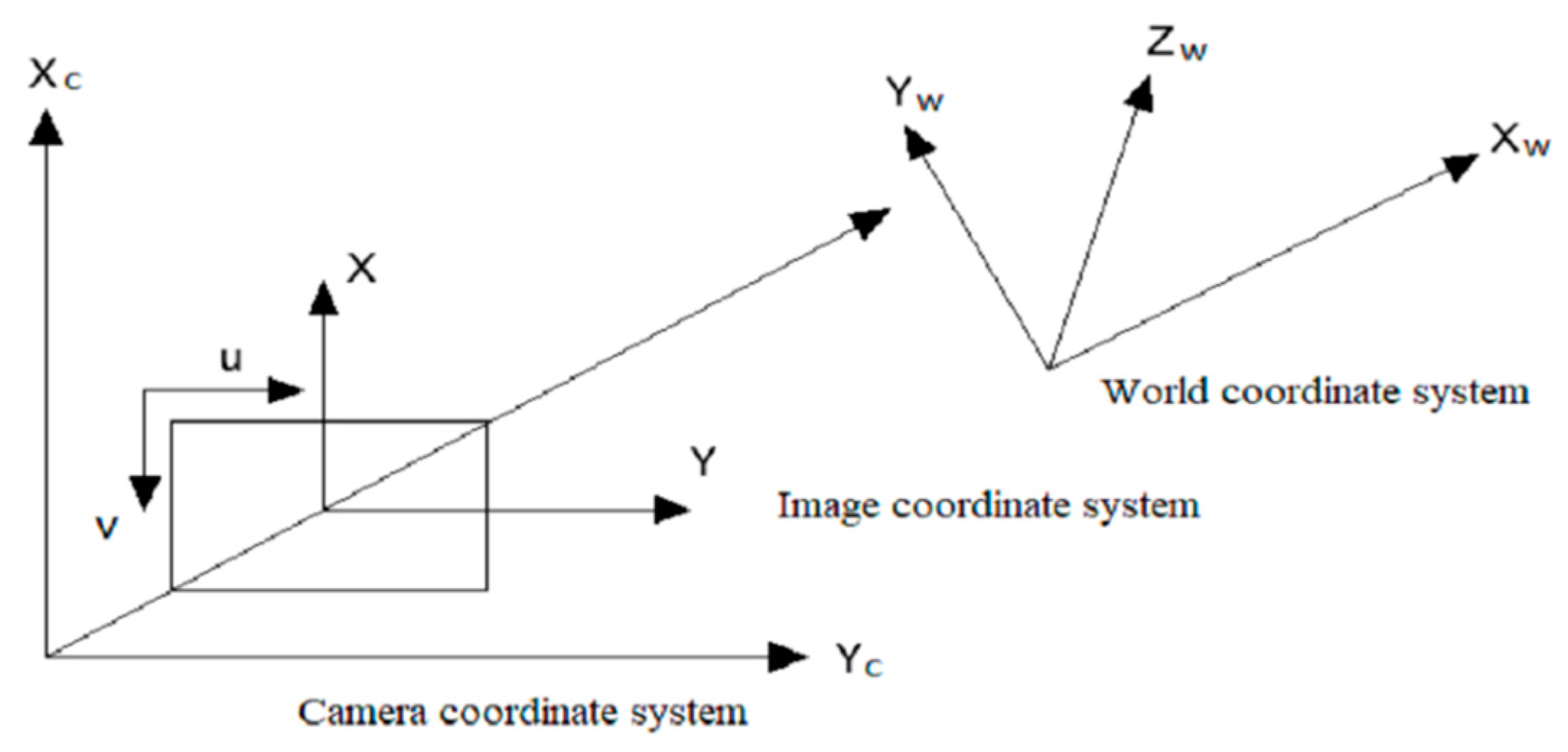
2.1. Camera Calibration
2.2. Accurate Estimation of the Internal and External Parameter Matrix
3. Improved Stereo Calibration Plate and Resulting Calibration Method
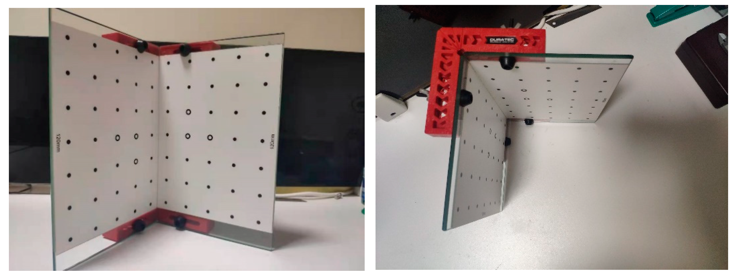
3.1. Structure of the Stereo Calibration Plate
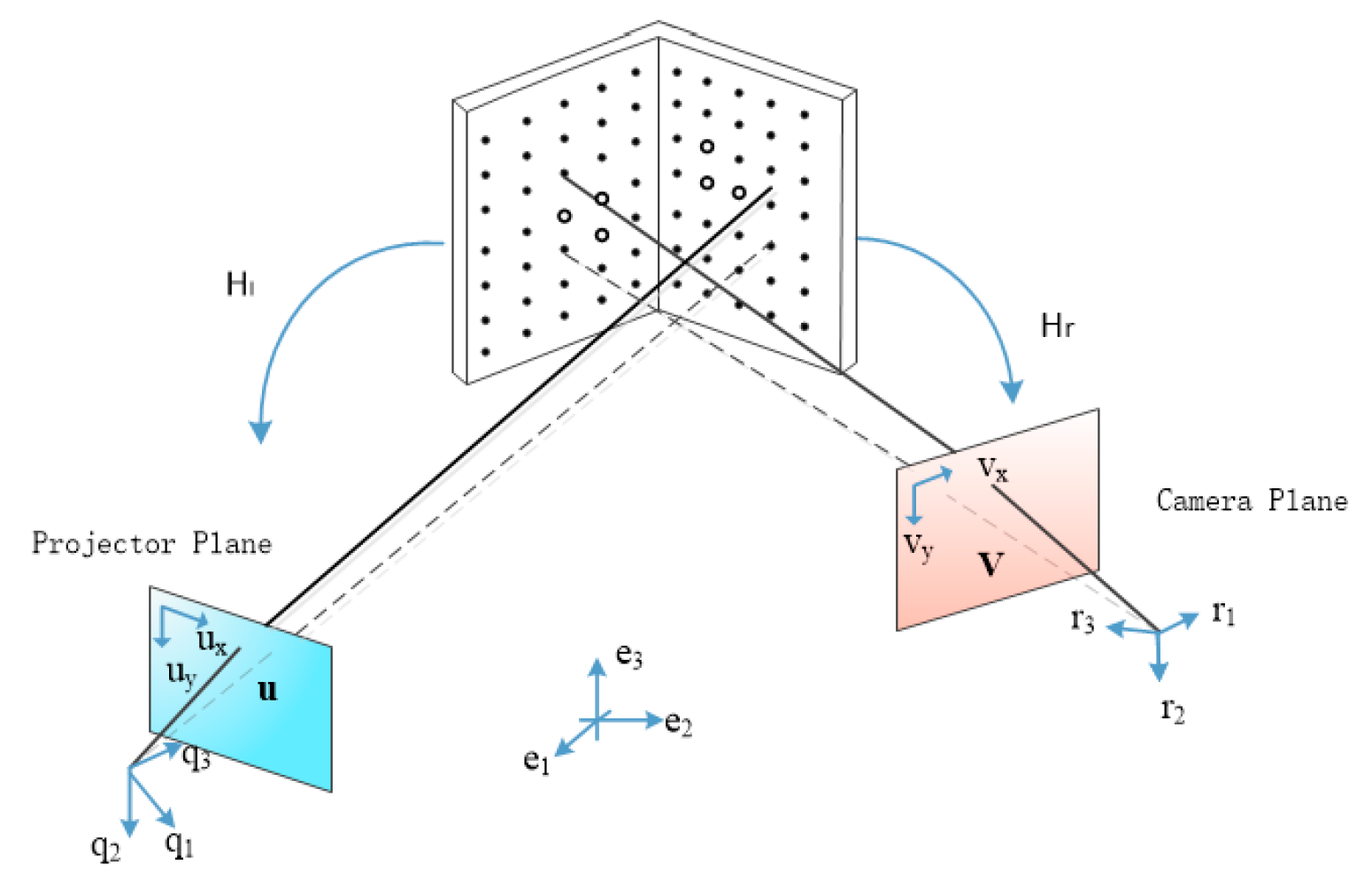
3.2. Homography Matrix from the Phase Plane to the Stereo Calibration Plate Plane
4. Experimental Results and Analysis
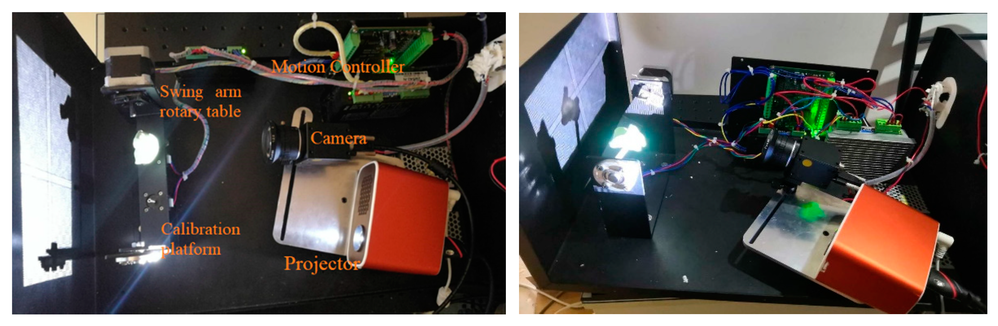
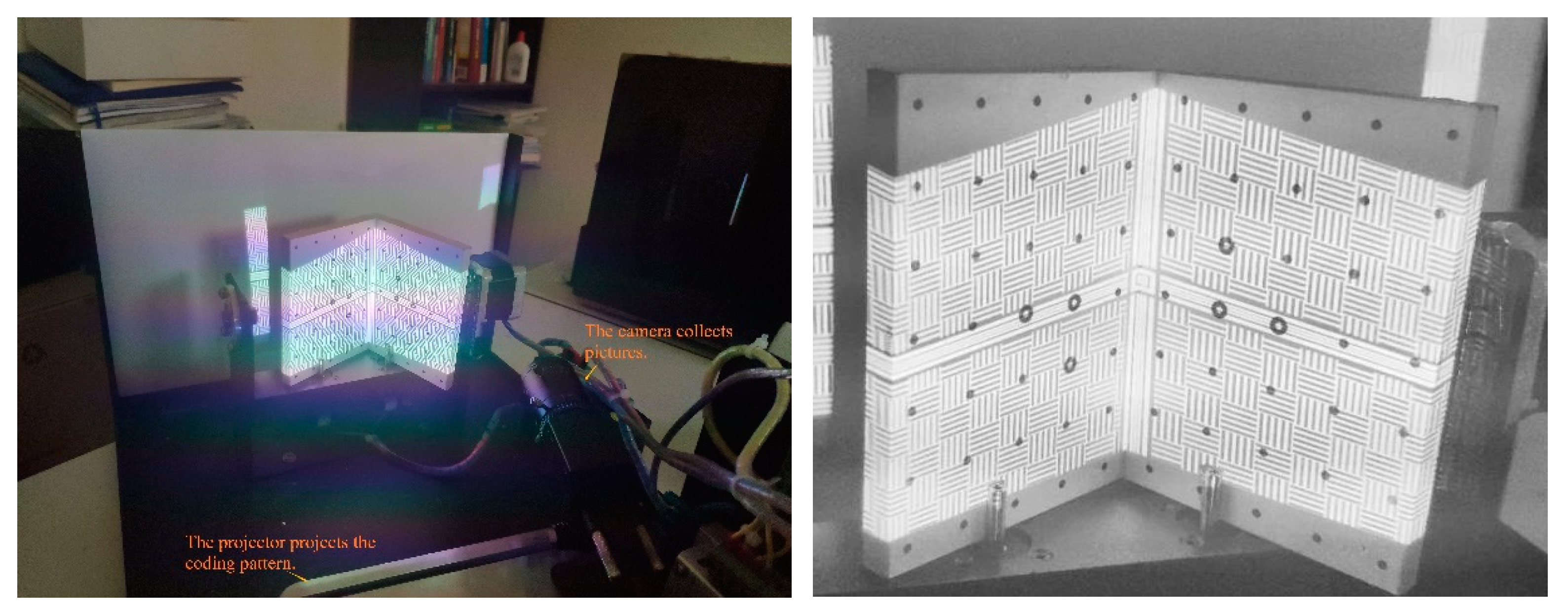
4.1. Experimental Layout
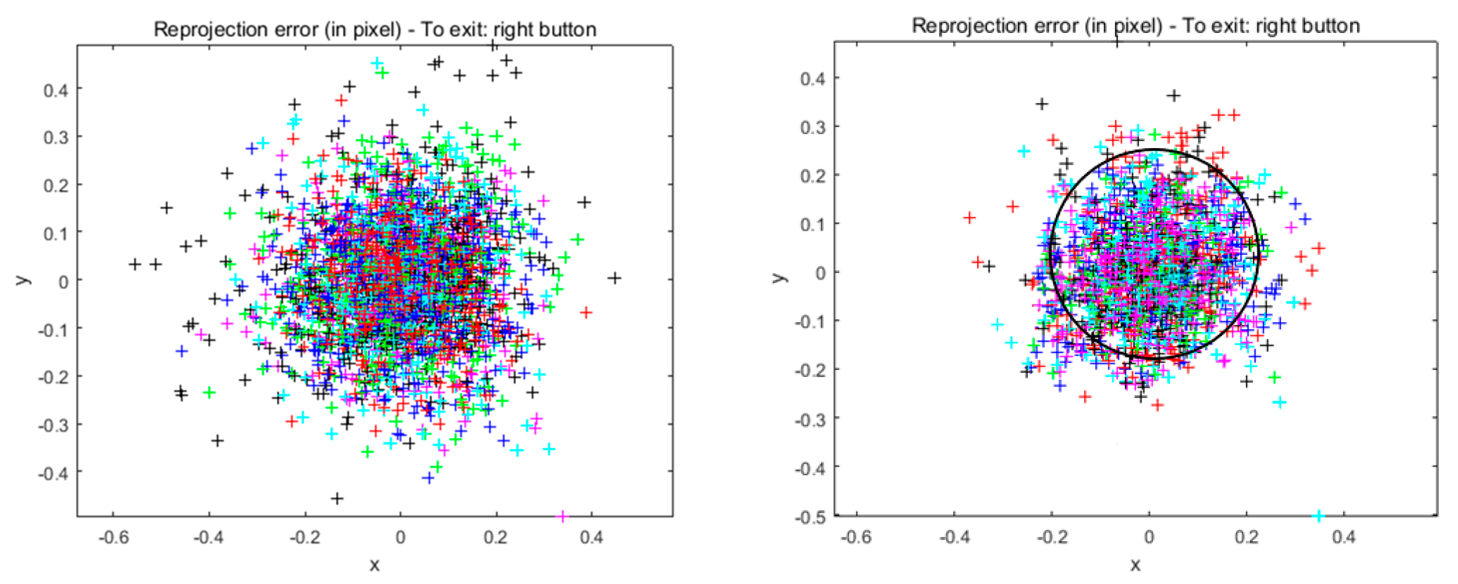
4.2. Stereo-Calibration Results
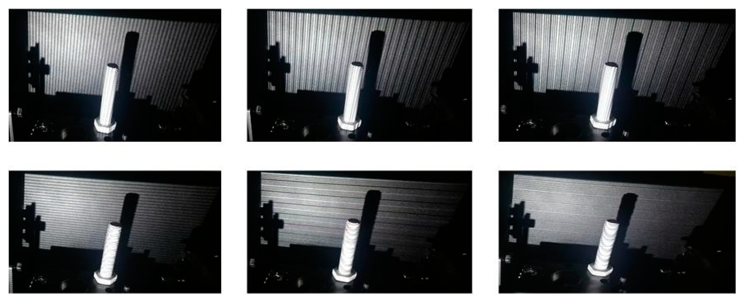
4.3. Three Dimensional-Surface Reconstruction Results
5. Conclusions
Author Contributions
Funding
Conflicts of Interest
References
- Hao, X.Y.; Li, H.B.; Shan, H.T. Stratified Approach to Camera Auto-calibration Based on Image Sequences. J. Geomat. Sci. Technol. 2007, 24, 5–9. [Google Scholar]
- Song, Z.; Qin, X.I.; Songlin, L.I.U. Joint Calibration Method of 3D Laser Scanner and Digital Camera Based on Tridimensional Target. J. Geomat. Sci. Technol 2012, 29, 430–434. [Google Scholar]
- Gao, Y.; Villecco, F.; Li, M.; Song, W. Multi-Scale Permutation Entropy Based on Improved LMD and HMM for Rolling Bearing Diagnosis. Entropy 2017, 19, 176. [Google Scholar] [CrossRef] [Green Version]
- Tsai, R.Y. A versatile camera calibration technique for high-accuracy 3D machine vision metrology using off-the-shelf TV cameras and lenses. IEEE J. Robot. Autom. 2003, 3, 323–344. [Google Scholar] [CrossRef] [Green Version]
- Zhang, Z.Y. A Flexible New Technique for Camera Calibration. IEEE Trans. Pattern. Anal. Mach. Intell. 2000, 22, 1330–1334. [Google Scholar] [CrossRef] [Green Version]
- Li, F.; Sekkati, H.; Deglint, J.; Scharfenberger, C.; Lamm, M.; Clausi, D.; Zelek, J.; Wong, A. Simultaneous Projector-Camera Self-Calibration for Three-Dimensional Reconstruction and Projection Mapping. IEEE Trans. Comput. Imaging 2017, 3, 74–83. [Google Scholar] [CrossRef]
- Merner, L.; Wang, Y.; Zhang, S. Accurate calibration for 3D shape measurement system using a binary defocusing technique. Opt. Lasers Eng. 2013, 51, 514–519. [Google Scholar] [CrossRef]
- Li, B.; Karpinsky, N.; Zhang, S. Novel calibration method for structured-light system with an out-of-focus projector. Appl. Opt. 2014, 53, 3415–3426. [Google Scholar] [CrossRef] [PubMed]
- Peng, S.; Sturm, P. Calibration Wizard: A Guidance System for Camera Calibration Based on Modelling Geometric and Corner Uncertainty. In Proceedings of the IEEE/CVF International Conference on Computer Vision (ICCV), Seoul, Korea, 27 October–2 November 2019; pp. 1497–1505. [Google Scholar]
- Rojtberg, P.; Kuijper, A. Efficient Pose Selection for Interactive Camera Calibration. In Proceedings of the 2018 IEEE International Symposium on Mixed and Augmented Reality (ISMAR), Munich, Germany, 16–20 October 2018; pp. 31–36. [Google Scholar]
- Miao, M.; Hao, X.Y.; Liu, S.L. Automatic Extraction and Sorting of Corners by Black and White Annular Sector Disk Calibration Patterns. J. Geomat. Sci. Technol. 2016, 33, 285–289. [Google Scholar]
- Fang, X.; Da, F.P.; Guo, T. Camera calibration based on polar coordinate. J. Southeast Univ. 2012, 42, 41–44. [Google Scholar]
- Geng, J. DLP-Based Structured Light 3D Imaging Technologies and Applications. In Proceedings of the Emerging Digital Micromirror Device Based Systems and Applications III, International Society for Optics and Photonics, San Francisco, CA, USA, 26 January 2011; Volume 7932, pp. 8–9. [Google Scholar] [CrossRef]
- Finlayson, G.; Gong, H.; Fisher, R.B. Color Homography: Theory and Applications. IEEE Trans. Pattern Anal. Mach. Intell. 2019, 41, 20–33. [Google Scholar] [CrossRef] [PubMed] [Green Version]
- Liu, H.; Song, W.Q.; Li, M.; Kudreyko, A.; Zio, E. Fractional Lévy stable motion: Finite difference iterative forecasting model. Chaos Solitons Fractals 2020, 133, 109632. [Google Scholar] [CrossRef]
- Huang, Y.H. A method for image denoising based on new wavelet thresholding function. Transducer Microsyst. Technol. 2011, 9, 76–78. [Google Scholar]
- Song, W.Q.; Cattani, C.; Chi, C.H. Multifractional Brownian Motion and Quantum-Behaved Particle Swarm Optimization for Short Term Power Load Forecasting: An Integrated Approach. Energy 2020, 194, 116847. [Google Scholar] [CrossRef]
- Wang, H.Y.; Song, W.Q.; Zio, E.; Wu, F.; Zhang, Y.J. Remaining Useful Life Prediction for Lithium-ion Batteries Using Fractional Brownian Motion and Fruit-fly Optimization Algorithm. Measurement 2020. [Google Scholar] [CrossRef]
- Song, W.Q.; Cheng, X.X.; Zio, C.C. Multifractional Brownian Motion and Quantum-Behaved Partial Swarm Optimization for Bearing Degradation Forecasting. Complexity 2020, 1–9. [Google Scholar] [CrossRef]


| Matrix | The Left Plane of the 3D Object | The Right Plane of the 3D Object |
|---|---|---|
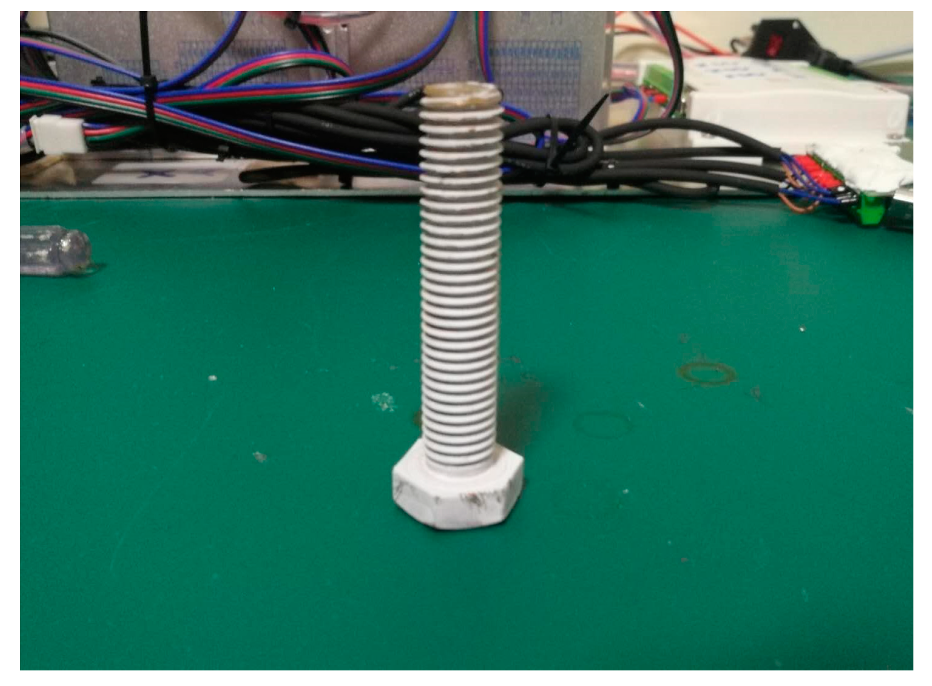
| Screw | Length (mm) | Head Thickness (mm) | Hex Diameter (mm) | Tooth Pitch (mm) |
|---|---|---|---|---|
| Standard parameters | 64.0 | 10.0 | 1.9 | 1.25 |
| Reconstruction parameters | 64.03 | 10.04 | 1.95 | 1.23 |
© 2020 by the authors. Licensee MDPI, Basel, Switzerland. This article is an open access article distributed under the terms and conditions of the Creative Commons Attribution (CC BY) license (http://creativecommons.org/licenses/by/4.0/).
Share and Cite
Li, M.; Liu, J.; Yang, H.; Song, W.; Yu, Z. Structured Light 3D Reconstruction System Based on a Stereo Calibration Plate. Symmetry 2020, 12, 772. https://doi.org/10.3390/sym12050772
Li M, Liu J, Yang H, Song W, Yu Z. Structured Light 3D Reconstruction System Based on a Stereo Calibration Plate. Symmetry. 2020; 12(5):772. https://doi.org/10.3390/sym12050772
Chicago/Turabian StyleLi, Meiying, Jin Liu, Haima Yang, Wanqing Song, and Zihao Yu. 2020. "Structured Light 3D Reconstruction System Based on a Stereo Calibration Plate" Symmetry 12, no. 5: 772. https://doi.org/10.3390/sym12050772
APA StyleLi, M., Liu, J., Yang, H., Song, W., & Yu, Z. (2020). Structured Light 3D Reconstruction System Based on a Stereo Calibration Plate. Symmetry, 12(5), 772. https://doi.org/10.3390/sym12050772