Spontaneous Chiral Symmetry Breaking and Entropy Production in a Closed System

Abstract

In this short article, we present a study of theoretical model of a photochemically driven, closed chemical system in which spontaneous chiral symmetry breaking occurs. By making all the steps in the reaction elementary reaction steps, we obtained the rate of entropy production in the system and studied its behavior below and above the transition point. Our results show that the transition is similar to a second-order phase transition with rate of entropy production taking the place of entropy and the radiation intensity taking the place of the critical parameter: the steady-state entropy production, when plotted against the incident radiation intensity, has a change in its slope at the critical point. Above the critical intensity, the slope decreases, showing that asymmetric states have lower entropy than the symmetric state.

1. Introduction

Modern thermodynamics, formulated in the 20th century by Onsager [1], De Donder [2], Prigogine [3,4], and others, introduced a critical concept lacking in its classical formulation: rate of entropy change and its relationship to irreversible processes. Classical thermodynamics was concerned with functions of state, such as energy and entropy, and their change from one equilibrium state to another. Absent from this theory of states is consideration of the rates of processes. Changes in entropy for infinitely slow reversible processes are calculated using the relation dS = dQ/T, (in which dS is the change in entropy, T is the temperature in Kelvin, and dQ is the heat exchanged between a system and its exterior). However, for changes that take place in a finite time due to irreversible processes, the theory does not specify a way of calculating the entropy change; it is only stated that dS > dQ/T. Modern thermodynamics is a theory of processes in which thermodynamic forces and the flows they drive are identified and the rate of entropy production is expressed in terms of these thermodynamic forces and flows [5,6]. More specifically, the rate of entropy production per unit volume, σ, is expressed in terms of the forces and flows as

$$\sigma =\frac{ds}{dt}={\displaystyle {\sum }_k}{F}_k{J}_k$$

(1)

in which s is the entropy density, F_k are the thermodynamic forces and J_k are thermodynamic flows. A temperature gradient, for example, is the thermodynamic force, F_k, that drives thermodynamic flow, J_k, of heat current. The force that drives chemical reactions has been identified as affinity [2,5,6] and the corresponding flow is the rate of conversion form reactants to products. This flow is expressed as the time derivative dξ/dt (mol/s) of the extent of reaction ξ [5,6]. For an elementary chemical reaction step, the rate of entropy production can be written in terms of the forward reaction rate, R_f, and the reverse reaction rate, R_r [6]

$$\sigma =R\left(R_f-R_r\right)\ln \left(\frac{R_f}{R_r}\right)$$

(2)

in which R is the gas constant. The total entropy production for a sequence of reactions is the sum of entropy productions of each reaction (indexed by k) [6]

$$\sigma =R{\displaystyle {\sum }_k}\left(R_{kf}-R_{kr}\right)\ln \left(\frac{R_{kf}}{R_{kr}}\right)$$

(3)

We note that calculations of entropy production using the above formulas require that the reverse reaction rates, R_r, are non-zero. In considering kinetic equations of a chemical system, often the reverse rates have high reaction barriers and, correspondingly, very low reaction rates, and are assumed to be “zero” because they are negligible compared to the forward rates. Low reverse reaction rates keep the system from evolving to equilibrium state. In the model we will present below, the system is driven far from equilibrium by an inflow of radiation. In the absence of radiation, our system evolves to equilibrium—there are no very high reaction barriers to keep it from reaching its equilibrium state.

It is well known that nonequilibrium chemical systems can undergo spontaneous symmetry-breaking transitions to organized structures called dissipative structures [6,7]. The large class of dissipative structures includes spatial patterns, chemical clocks, and structures with chiral asymmetry. These structures arise when a nonequilibrium system becomes unstable and undergoes a transition to new organized state. The model we present below shows a chiral symmetry breaking transition to an asymmetric state as the intensity of radiation increases.

The study of spontaneous chiral symmetry breaking in chemical systems has a long history, starting in the 1950s with the first model by Frank [8]. In the 1970s, when the theory of dissipative structures was developed, instability, bifurcation, and spontaneous symmetry breaking in non-equilibrium systems became the foundation for the study of chiral asymmetry we see in nature [4,7,9,10,11]. A general theory of chiral symmetry breaking in chemical systems, independent of the details of the chemical kinetics, was formulated, and it was used to study the sensitivity of chiral symmetry breaking systems to small chiral influences [11,12,13]. Using this theory, it was possible to calculate the time scales needed for a chiral-symmetry-breaking chemical system to be influenced by the chiral asymmetry of electro-weak interaction in molecules [14], and it was found that this timescale is of the order to 10⁴ years [15]. These results show that a lot of interesting and important general conclusions can be arrived at through using theoretical models [16,17]. Along these lines, we investigate the thermodynamic aspects of systems that spontaneously break chiral symmetry, using a model presented below.

Using nonequilibrium thermodynamics, we analyze the behavior of entropy production, σ, for a reaction scheme that consists of a photochemically driven closed system (that has no flow of matter). The incident radiation drives a generation–decomposition cycle of chiral molecules. At the critical intensity (above which the system breaks chiral symmetry), the slope of the rate of entropy production, σ, changes just as entropy does in a second-order phase transition. We have reported a similar result in a flow system with an inflow of reactants and outflow of products [18]. There is a basic difference, however: in our previous study, the slope of σ increased, but in our current study we find that the slope decreased, although in both cases the behavior of σ is similar to that in a second-order phase transition.

2. Materials and Methods

All reactions in our scheme are reversible so that the system can reach a state of chemical equilibrium. At equilibrium, the rate of entropy production is zero. The reaction scheme of this photochemically driven closed system is shown in

Table 1. A model photochemically driven reaction scheme in a closed system. The table lists all the elementary steps in the model. The excitation of T to the state TE drives the reaction that generate chiral species X_L and X_D. Reactions R4a, R4b, R5a, R5b are the autocatalytic steps for X_L and X_D. Autocatalysis and reaction R6 result in spontaneous breaking of chiral symmetry when the intensity of radiation, II, is above a critical intensity, II_C.

Chemical Reactions	Number
S + II ⇄ TE	(R1)
T ⇄ TE	(R1a)
S + TE ⇄ XL	(R2)
S + TE ⇄ XD	(R3)
S + XL ⇄ SL	(R4a)
SL + TE ⇄ 2XL	(R4b)
S + XD ⇄ SD	(R5a)
SD + TE ⇄ 2XD	(R5b)
XL + XD ⇄ P + W	(R6)
P ⇄ 2S	(R7)
W ⇄ 2T	(R8)

. It is assumed to take place in a homogeneous aqueous phase in which radiation is incident. For a photochemical reaction, the intensity of a narrow band of wavelength is the relevant intensity, therefore it will have a low value compared to a typical intensity of blackbody radiation that includes all wavelengths—for example, radiation from the sun. An achiral molecule, T, is photochemically activated to an excited species or a more reactive isomer, TE, as shown in reaction (R1); II is the intensity of radiation of the exciting wavelength. TE can radiate its excitation energy and return to the unexcited state, T (R1a), through various processes. During the transition of TE to T, the emitted radiation undergoes scattering and thermalizes to the temperature of the system. (R1a) represents all the processes that keep TE and T at equilibrium (including thermal radiation [6]) in the absence of external radiation. In writing the reaction rates for T and TE, we only need to include additional term in the forward reaction that includes II and the all reverse reactions, TE to T, combined into one reaction rate. The excited species TE can also react with an achiral molecule S to form a chiral species, X_L or X_D (R2 and R3). The set of reactions R4a and R4b are elementary steps of an autocatalytic reaction for X_L with the intermediate species S_L; similar reaction steps result in the autocatalytic production of X_D, as shown in R5a and R5b. Reaction steps R6, R7 and R8 show reactions through which the species decompose into starting material S and T. The scheme explicitly has all the steps needed for the system to reach chemical equilibrium in the absence of radiation.

The above model is a variation of the models in our earlier studies [11,12,15] which are modifications of the original model of Frank [8]. The modifications allow us to analyze non-equilibrium symmetry breaking and rate of entropy production. Models such as this are used to extract general properties that are not model dependent. Examples of such properties are the qualitative behavior of steady-state rate of entropy production as a function of a parameter that drives the system away from equilibrium (such as the incident radiation intensity II in the above model). The difference in concentration between enantiomers of a chiral species as a function of a parameter, such as the intensity II, is generally parabolic, as predicted by bifurcation theory based on the symmetry group (mirror symmetry in this case) of the system, regardless of the details of the chemical reactions that break chiral symmetry.

Though there is currently no known reaction that has all the properties in the above model, the reaction has no steps that are implausible. For example, reactions (R1), (R1a), (R2) and (R3) comprise a photoaddition reaction that produces a chiral compound. An example is the following reaction series [19,20]:

(Ph)2 C = CH(R1) + hv → [(Ph)2 C = CH(R1)]*	(R9)
[(Ph)2 C = CH(R1)]* + (R2)OH → [(Ph)2 HC − CH(R1)(OR2)]L	(R10)
[(Ph)2 C = CH(R1)]* + (R2)OH → [(Ph)2 HC − CH(R1)(OR2)]D	(R11)

in which Ph is the phenyl group and R¹ = CH₃ or C₂H₅ and R² = CH₃, C₂H₅ or C₃H₇. In the reaction (R9), a photon is absorbed by the electrons in the C=C double bond and the molecule transitions to a reactive excited state [(Ph)₂ C = CH(R¹)]*. In the addition reaction shown in (R10) and (R11), the excited molecule reacts with an alcohol, (R²) OH, and produces a chiral compound (Ph)₂ HC − CH(R¹)(OR²) in the L and D enantiomeric forms. In this compound, the carbon shown in boldface is a chiral carbon (its tetrahedral bonds to four different groups makes it so). Other examples of photoaddition reactions producing chiral products from achiral reactants can be found in [19]. We note that TE need not be an excited state; it could be a different, more reactive isomer of the T [19].

The reactions (R4a)–(R5b) are steps leading to chiral autocatalysis. This involves the formation of a chiral complex of S and X in their enantiomeric forms. Examples of chiral complexes resulting in reactions with a high degree of chiral selectivity have been known for a long time [21,22]. In an article published in 1984, we noted some mechanisms that are based on chiral ligands in rhodium phosphine catalysts which could lead to chiral autocatalysis [12,22]. To date, there are several chirally autocatalytic reactions that have been experimentally studied. Chiral symmetry breaking was noticed and systematically studied first in NaClO3 in 1990 [23], and in 1995 chiral autocatalysis and amplification of small initial enantiomeric excess was reported in inorganic reactions involving cobalt complexes [24] and in organic reactions involving alkylation of aldehydes [25]. Since then, these and closely related systems have been extensively experimentally studied and the mechanisms of chiral autocatalysis have been investigated [26,27,28,29,30,31]. A variant of chiral symmetry breaking in stirred crystallization was reported in 2005, and it too has been studied extensively [32,33]. The mechanisms of chiral autocatalysis vary in these systems: in crystallization, it is secondary nucleation, in the organic and inorganic reactions, cluster/complex formation seems to be involved. Reactions (R4a) and (R5a) may be thought of as a simple form of chiral complex formation. As was noted in a review [27], the exact details of chiral catalysis are not of significance for the general properties symmetry-breaking bifurcation and thermodynamic properties of such systems. In particular, properties such as phase-transitions-like behavior we present here are quite independent of the details of chemical kinetics. Examples of reaction (R6), the dimer formation of enantiomers, are also known; in fact, such dimerization of certain chiral catalysts leads to asymmetric amplification [34].

For the above theoretical model (R1)–(R8), the corresponding forward and reverse rate for each reaction are written as follows, in which concentrations are shown explicitly as functions of time:

R1f = (k1f + k1 II)T[t], R1r = k1r TE[t]

(4)

R2f = k2f S[t] TE[t], R2r = k2r X_L[t]

(5)

R3f = k3f S[t] TE[t], R3r = k3r X_D[t]

(6)

R4af = k4af S[t] X_L[t], R4ar = k4ar S_L[t]

(7)

R4bf = k4bf S_L[t] TE[t], R4br = k4br (X_L[t])²

(8)

R5af = k5af S[t] X_D[t], R5ar = k5ar S_D[t]

(9)

R5bf = k5bf S_D[t] TE[t], R5br = k5br (X_L[t])²

(10)

R6f = k6f X_L[t]X_D[t], R6r = k6r P[t]W[t]

(11)

R7f = k7f P[t], R7r = k7r (S[t])²

(12)

R8f = k8f W[t], R8r = k8r (T[t])²

(13)

In these equations, the rate constants are written as k1f, k1r etc., and the concentration are written as T[t], S[t], etc. In terms of these forward and reverse rates, the rate equations for the concentrations can be written as:

d T[t]/dt = −R1f + R1r + 2R8f − 2R8r

(14)

d TE[t]/dt = −R1f + R1r − R2f + R2r − R3f + R3r − R4bf + R4br − R5bf + R5br

(15)

d S[t]/dt = −R2f + R2r − R3f + R3r –R4af + R4ar − R5af + R5ar + 2R7f − 2R7r

(16)

d S_L[t]/dt = R4af − R4ar − R4bf + R4br

(17)

d S_D[t]/dt = R5af − R5ar − R5bf + R5br

(18)

d X_L[t]/dt = R2f − R2r − R4af + R4ar + 2R4bf − 2R4br − R6f +

(19)

d X_D[t]/dt = R3f − R3r − R5af + R5ar + 2R5bf − 2R5br − R6f + R6r

(20)

d P[t]/dt = R6f − R6r − R7f + R7r

(21)

d W[t]/dt = R6f − R6r − R8f + R8r

(22)

This set of coupled non-linear equations were solved numerically using Mathematica NDSolve. NDSolve is a Mathematica command that has the following structure: NDSolve[{Equations}, {y_i},{t, t_min, t_max}], in which “Equations” are the differentials equations for the set of functions {y_i} with t as the independent variable; numerical solutions are obtained in the range t_min, to t_max. More details can be found in the online documentation that comes with Mathematica. The rate constants used for the numerical solutions are summarized in Figure 1. In assigning values to rate constants, there are consistency conditions that must be met. For example, since reactions (R4a) and (R4b) together are equivalent to (R2), the products of the equilibrium constants of R4a and R4b must equal the equilibrium constant of R2. This gives us the following condition for the rate constants:

(k4af/k4ar)(k4bf/k4br) = k2f/k2r

(23)

Numerical values were assigned to rate constants so as to fulfill these requirements. The units were chosen so that all concentrations are in mol/L. Assigned numerical values are such that the concentrations of the reactants have realistic values. Symmetric (racemic) and asymmetric states are parametrized by α = (X_L − X_D), in the symmetric state α = 0 and in the asymmetric state α ≠ 0.

3. Results

The rate equations were first solved for an equilibrium state where the incident radiation intensity, II, was set to 0. The initial concentrations of species S and T were set to 0.01 M and the initial concentrations of all other species were set to 0.0 M. Under these conditions, the system evolves to its racemic equilibrium state, in which α = 0.

The simulation code was run for sufficient time (about 10⁴ s) to ensure the concentrations of all species have reached a steady state, which is the equilibrium state. At t = 10⁴ s, the concentrations at equilibrium were: S = T = 8.478 × 10⁻³ M, TE = 8.477 × 10⁻⁶ M, S_L = S_D = 3.047 × 10⁻⁶ M, X_L = X_D = 3.593 × 10⁻⁵ M, and P = W = 7.188 × 10⁻⁴ M. The conversion of the initial species S and T compared to other species was rather small for the numerical values of the rate constants shown in Figure 1. By choosing a different set of rate constants, the conversion could be increased. The numerical values confirm that complete symmetry of the system was maintained when no incident radiation is present. 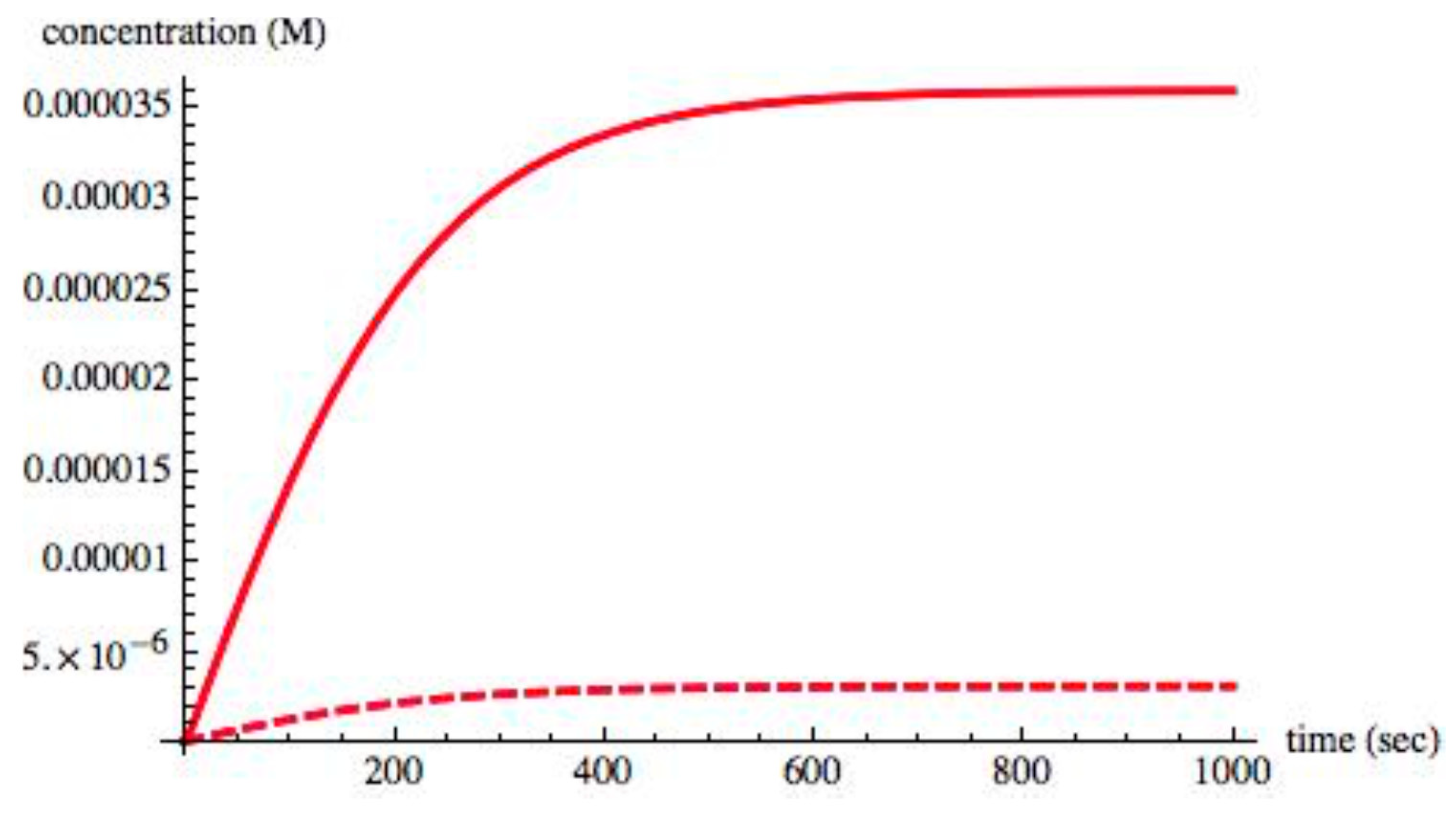Figure 2 shows the time evolution of the chiral species S_L, S_D, X_L, X_D from t = 0 s, to t = 1000 s. As the system evolved to its equilibrium state, the entropy production σ was monitored; initially, it took a nonzero value but, as expected, its value decreased to zero at the equilibrium state.

We then used these values for a symmetric equilibrium state as initial values for a system subject to a radiation input, i.e., II > 0. This radiation input serves as a means to push the system away from thermodynamic equilibrium. A very small excess, about 0.1% (3 × 10⁻⁸ M) of X_L was introduced into the system as a “random fluctuation”. If the system has the mechanism to break chiral symmetry, it will have a critical value II_C. At values of II < II_C, this excess 0.1% of X_L will decrease and the system will again evolve into a steady state where X_L = X_D; at values of II > II_C, the excess will increase and lead to a steady state in which X_L > X_D. In a real system, this slight perturbation may be due to a random fluctuation such as a local excess of one enantiomer that may then be amplified, resulting in a state of broken symmetry. The overall behavior of the system is summarized in Figure 3.

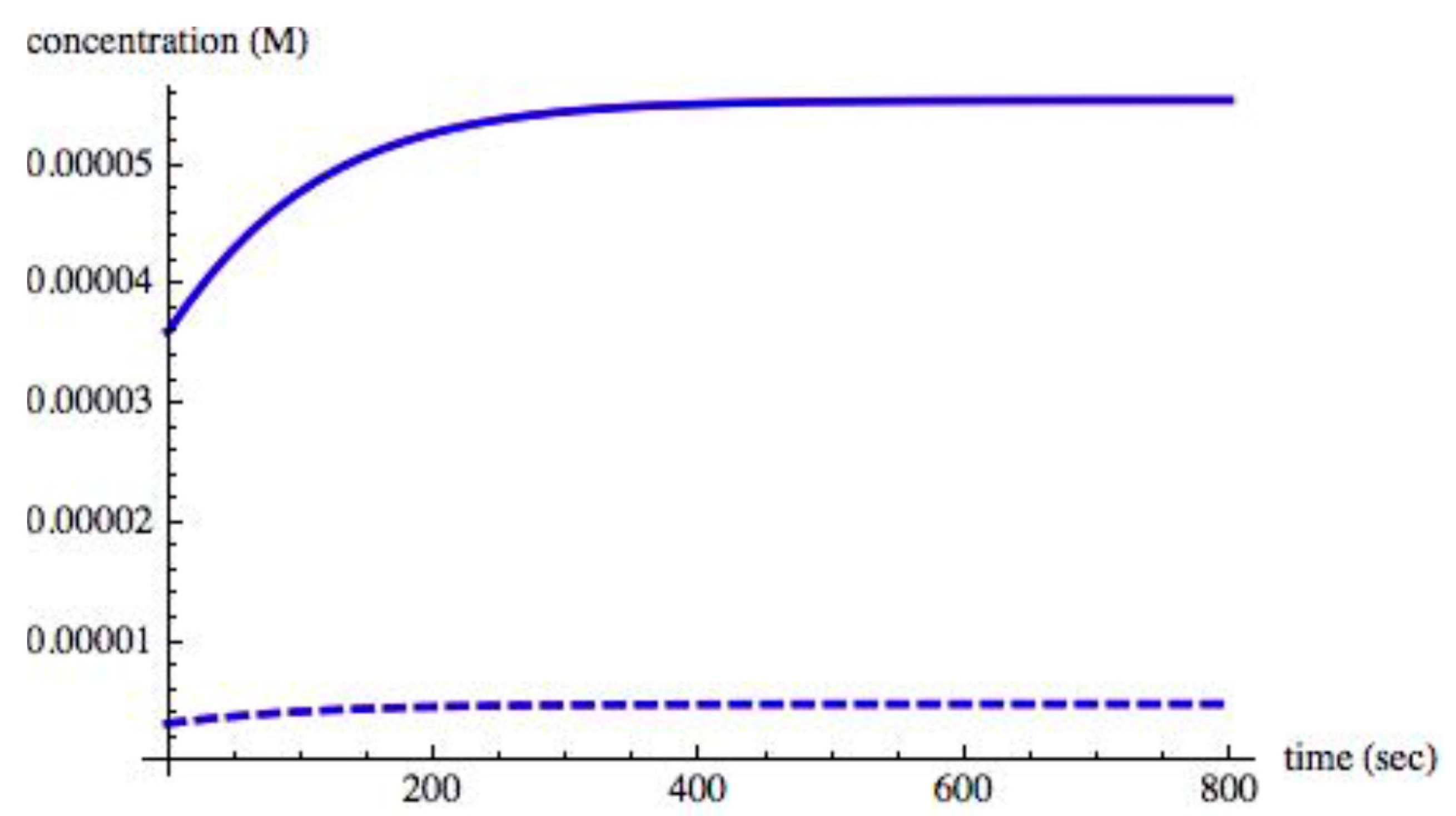
It was found that this system indeed has the mechanism needed for breaking chiral symmetry. At values of II < 0.004, the system evolved to a symmetric state corresponding to X_L = X_D and α = 0. Figure 4 shows the time evolution of the chiral species when II = 0.0030. A steady state is reached in approximately 600 s.

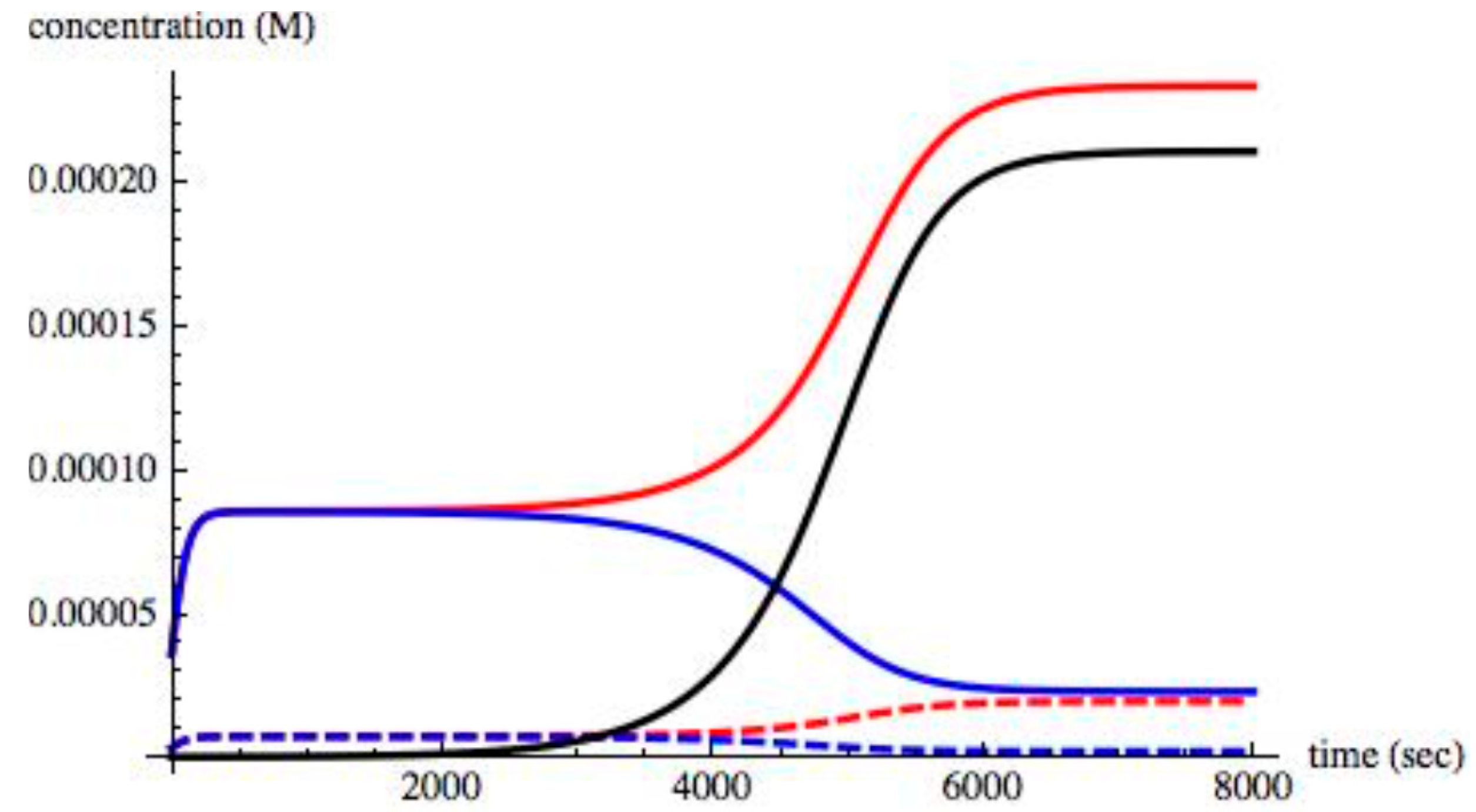
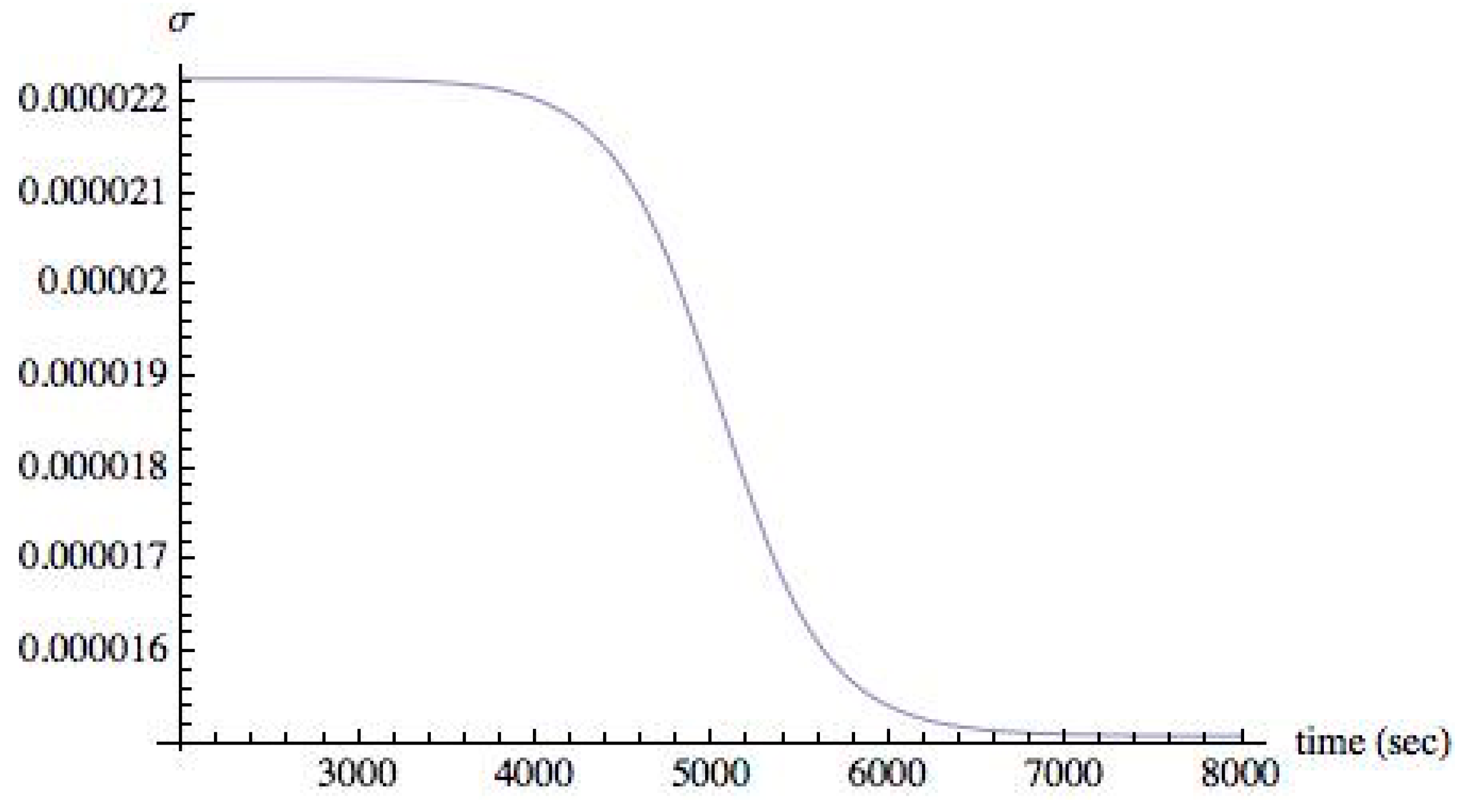
For values of II > 0.004, the small excess of 0.1% of XL in the initial concentration increased, thus driving all chiral species to an asymmetric state. A time evolution of the chiral species in an asymmetric state when II = 0.008 is shown in Figure 5.

As shown, steady state is reached about 7000 s. The time taken to reach steady state, the relaxation time, depends on the value of II and on the amount of initial excess (0.1% of X_L). As is well known in the study of stability of steady states [6,7,9], the initial exponential growth of the small enantiomeric excess depends on the eigenvalue of the unstable mode of the linearized equations derived from the set (14)−(22) around the initial state. These linearized equations are obtained by assuming a small perturbation of the concentrations, δC_k, from the initial steady state. This leads to a set of linear equations of the type dδC_k /dt = Σ_l L_klδC_l [6,7,9]. The eigenvalues of L_kl with positive real parts are the exponents that determine the initial rate of growth of the enantiomeric excess. However, the later growth and leveling off at the steady state depend on the kinetics and rate constants. In general, near the critical point II_C, the relaxation time is long, the so-called “critical slowing”, but as the value of II increases, the growth rate becomes faster and the relaxation time decreases.

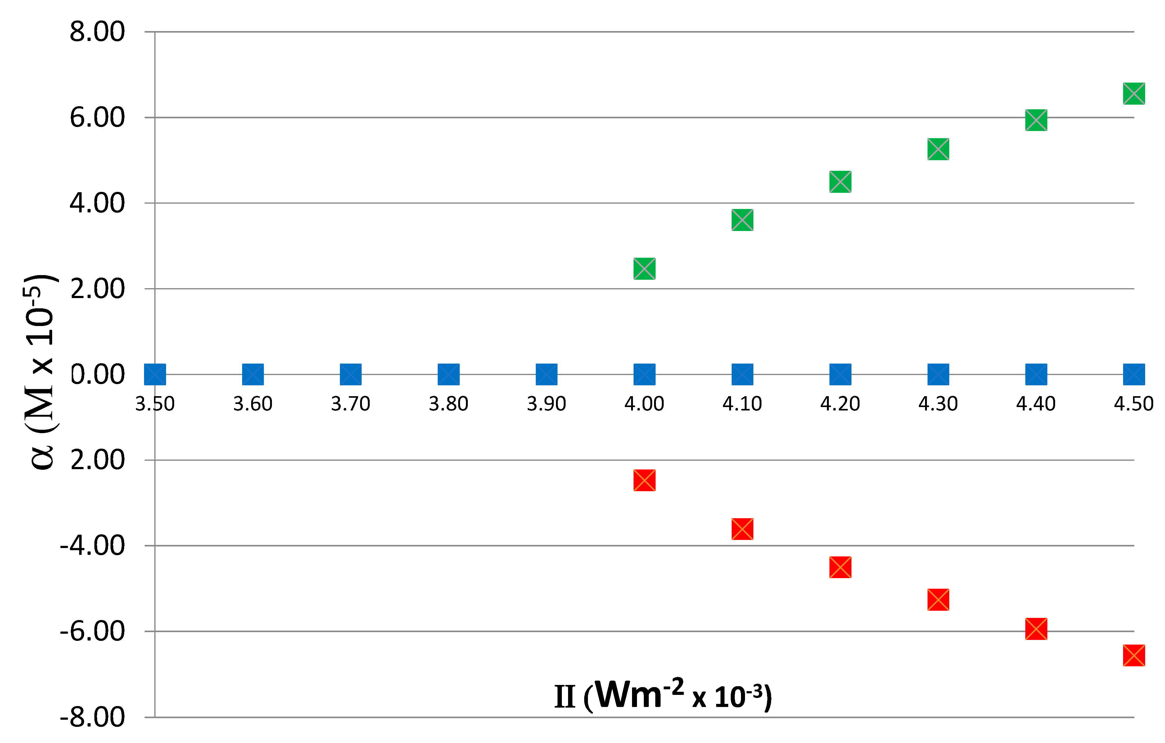
To determine the relation between the steady-state value of α on II, the reaction was run for various values of II, from 0.0035 to 0.0045, and the corresponding steady-state values of α were obtained. As noted above, the time it takes for the system to reach an asymmetric steady state depends on the value of II; close to the critical value II_C (0.004 in this case), the relaxation to asymmetric steady state is slower and it becomes faster as the value of II increases. The exact quantitative relationship between relaxation time and II depends on the kinetics and rate constants and not of significance to the current study. In these runs, to obtain both positive and negative branches of α, the initial condition with a 0.1% excess of X_D was also included. The dependence of α on II is shown in Figure 6, demonstrating the typical bifurcation of asymmetric states above the critical value II_C = 0.004. As is expected, in a chiral symmetry breaking transition, the values of α above the critical point are parabolic.

With these results, we now turn to the rate of entropy production σ. As stated above, initially the system is in the state of equilibrium, with the intensity of radiation II = 0 and σ = 0. Then the intensity of the radiation II is increased to a non-zero value and the rate of entropy production σ is monitored. Initially, σ sharply increases and, as the system reaches its steady-state, corresponding to the set value of II, the entropy production also reaches its steady state value. Figure 7 shows the evolution of σ from its value when t = 0, to its final steady-state value when II = 0.008. The final steady state value of σ is small compared to its initial value, but it is nonzero.

We would like to note that the results shown above do not depend crucially on the particular values assigned to rate constants. Whether symmetry breaking occurs or does not depends mostly on the mechanism of reactions in the model, not on a narrow range of values of rate constants. In general, qualitative properties change drastically due to small changes in rate constants only in singular cases. The presented model is not singular. In our study, we have tried a range of rate constants and observed symmetry breaking. A typical value is presented in this article.

Our objective is to study the behavior of σ as the intensity of radiation II moves form a value below to a value above the critical value II_C. In a previous study [18] of an open system, σ behaved as entropy does in a second order phase transition: its slope is discontinuous at the transition point. In addition, we noted that its slope increased above the critical point. This behavior was consistent with the Maximum Entropy Production (MEP) hypothesis [35,36,37,38,39,40] that states that non-equilibrium steady states maximize the rate of entropy production. In other words, the breaking of symmetry was a reflection of the general tendency of non-equilibrium systems and, from this point of view, it was only to be expected. This would imply that biochemical asymmetry is a consequence of MEP. To date, there is no general proof for MEP; indeed, in our own investigation we found that MEP was valid for some systems but not all. MEP, in general, is a controversial hypothesis and its applications to various complex systems have been questioned [41]. Hence, we investigated MEP in the context of chiral symmetry breaking.

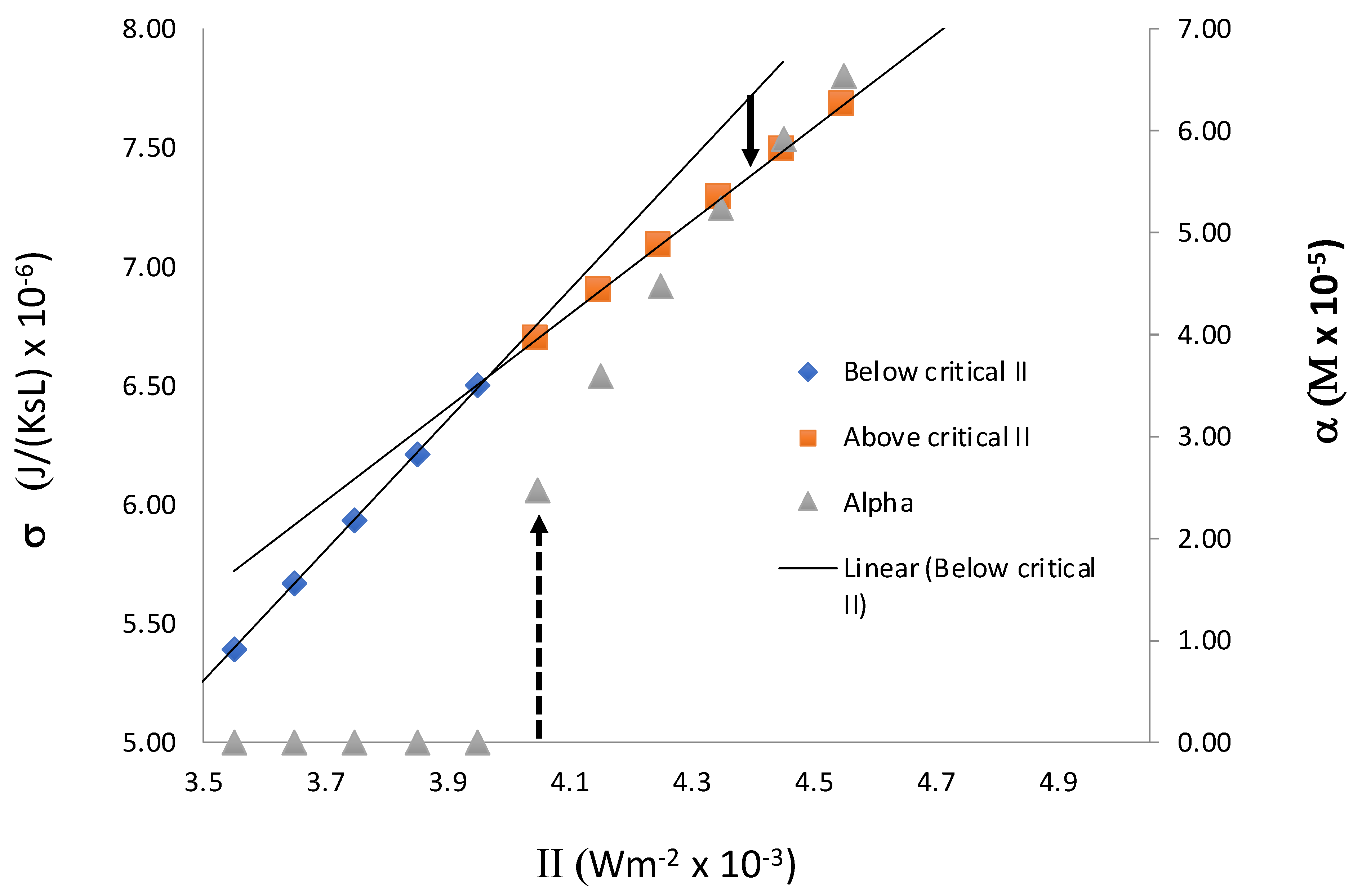
Figure 8 shows the behavior of entropy production in the closed system we present here. It shows a change in the slope at the transition point, IIC, as in our previous study. From the point of view of symmetry breaking transition, we see that entropy production behaves in a way that is similar to that of entropy in a second-order phase transition. However, unlike the previous result, the slope decreases above the critical point. As indicated in Figure 8, when II > II_C, if initially we set the system in a non-equilibrium symmetric state, which is an extrapolation of the symmetric state below II_C, the system evolves to an asymmetric state in which σ is lower. The extrapolation of the symmetric state beyond the critical value II_C is possible on a computer because, without a small perturbation in X_L or X_D, or other chiral species, the system stays in an unstable symmetric steady state. With a small perturbation, it evolves to the stable asymmetric state. The time evolution of the system from this initial state to its final asymmetric steady state results in the decrease in σ, thus indicating that the stable asymmetric state is associated with a lower value of σ compared with that of a symmetric state. Thus, we see that the entropy production in a closed system is not consistent with MEP, because MEP would predict higher values for σ in the asymmetric state.

4. Concluding Remarks

Our results show several aspects of chiral symmetry breaking. First, they show that Frank’s original model can be modified with several additional steps—all of which are possible elementary chemical reaction steps—to demonstrate that spontaneous chiral symmetry breaking can occur in a photochemically driven closed system. Our model is motivated by the fact that the earth is a essentially a closed system (except for a very small influx in interstellar matter such as meteorites) and the evolution of life was driven by incident solar radiation. The incident radiation drives a cycle of generation and decomposition of chiral compounds that, at a sufficiently high intensity of radiation, makes a transition to a state of broken chiral symmetry. This example demonstrates that life on earth could have evolved under such conditions of prebiotic molecular chiral asymmetry.

From a thermodynamic viewpoint, this study also confirms that chiral symmetry breaking transitions are similar to second-order phase transitions, with entropy production taking the place of entropy. We note that the general qualitative features of bifurcation of asymmetric states and change in the behavior entropy production at the critical point, shown in Figure 6 and Figure 8, are a consequence of the two-fold symmetry of the system, not the particularities of the chemical reactions in the model. In fact, using the system’s symmetry group, it is possible to derive the following generic equation for the evolution of α near the critical point: dα/dt = −Aα³ + Bα + C, in which A, B and C are functions of the kinetic constants of the chiral symmetry breaking chemical reactions [11,12,13,15]. Finally, we show that the behavior of entropy production in this chiral-symmetry-breaking system is not consistent with the MEP hypothesis, because MEP implies that the state of broken symmetry will have a higher rate of entropy production compared to a symmetric state, but we find the opposite to be the case in this model. In a system with an inflow of reactants and outflow of products, however, the entropy production was higher in the asymmetric state. This indicates that MEP is valid for a certain class of systems, but what this class is has not yet been clearly identified.