Abstract
Bi-level programming problem (BLPP) is an optimization problem consists of two interconnected hierarchical optimization problems. Solving BLPP is one of the hardest tasks facing the optimization community. This paper proposes a modified genetic algorithm and a chaotic search to solve BLPP. Firstly, the proposed algorithm solves the upper-level problem using a modified genetic algorithm. The genetic algorithm has modified with a new selection technique. The new selection technique helps the upper-level decision-maker to take an appropriate decision in anticipation of a lower level’s reaction. It distinguishes the proposed algorithm with a very small number of solving the lower-level problem, enhances the algorithm performance and fasts convergence to the solution. Secondly, a local search based on chaos theory has applied around the modified genetic algorithm solution. Chaotic local search enables the algorithm to escape from local solutions and increase convergence to the global solution. The proposed algorithm has evaluated on forty different test problems to show the proposed algorithm effectiveness. The results have analyzed to illustrate the new selection technique effect and the chaotic search effect on the algorithm performance. A comparison between the proposed algorithm results and other state-of-the-art algorithms results has introduced to show the proposed algorithm superiority.
1. Introduction
Optimization problems have classified into single-level optimization problems and multi-level optimization problems. In single-level optimization problems, there is just one decision-maker tries to find an optimal solution to an optimization problem [1,2]. In multi-level optimization problems, there are hierarchically nested optimization problems. Every optimization problem of these hierarchical nested systems has its decision-maker that tries to find his/her optimal solution [3,4]. Many applications appeared in the real-world in engineering design, traffic problems, problems, economic policy and so on are multi-level optimization problems [5,6,7,8,9]. Multi-level optimization problems consist of “N” optimization problems. The first problem is the upper-level problem. The leader is the upper-level decision-maker. The next problems are lower-level problems. The followers are the lower levels decision-makers. A leader knows the followers’ objective function and constraints while the followers may know or not leader’s objective functions and constraints. Leaders and followers are independent and often have conflicting objectives although their decisions affect each other. The hierarchical decision process starts when the leader takes his/her decisions. Then, the first follower takes his/her own decisions upon the leader’s decisions and so on for the remainder followers; every follower determines his/her own decisions upon his/her upper’s level decisions. The followers’ decisions affect the leader’s solution. Bi-level programming problems is a multi-level programming problem with two levels: upper-level programming problem and lower-level programming problem.
Researchers have given great attention to solving single-level optimization problems [10,11,12,13,14,15]. Bi-level programming problems haven’t gained the same attention. Small relatively studies shave proposed to handle bi-level programming problem (BLPP). The cause of the lack of studies is difficulties in solving such problems. Solving BLMPP needs to solve the lower-level programming problem to know the feasible space of the upper-level problem. Needing to solve the lower-level programming problem increases BLPP solution requirements. It produces difficulties in solving such as disconnectedness and non-convexity even to the simple problems. Such difficulties make BLPP is considered one of the strongly NP-hard problems [9]. BLPP solving techniques are divided into classical techniques and evolutionary techniques. Classical techniques are as descent direction method, best algorithm, exact penalty function etc. [10,11]. Classical techniques are limited to specified BLPP. It can treat only with convex differentiable problems. In [12] Liu et al. proposed a survey on multilevel optimization problems and its solution techniques. Lu et al. compare between different solution techniques and indicated that using classical techniques to solve BLPP isn’t available to various multilevel programming problems especially for large-scale problems and it can be used only to specified types of BLPP problems. Wang et al. introduced an evolutionary algorithm based on the classical technique for solving a special type of BLPP [13]. They present a genetic algorithm based on the simplex method for solving the linear-quadratic bilevel programming problem. Firstly, they apply Kuhn–Tucker conditions on the lower level programming to transform the problem a single level problem. Following this, they apply the genetic algorithm based on the simplex method on the single level problem. Their technique treats only with specified BLPP, linear-quadratic bi-level programming problem.
Evolutionary techniques are inspired by the natural behavior of molecular, biological, neurobiological systems and a swarm of insects, etc. Evolutionary techniques are as follows: simulated annealing, genetic algorithms, ant colony optimization, neural-network-based techniques and particle swarm optimization [14,15,16,17,18,19,20,21,22]. The evolutionary techniques have an advantage than classical methods that it can treat with a non-differentiable non-convex optimization problem. Sinha et al. in [23] illustrated that recently there has been an increasing interest in evolutionary algorithms in tackling BLPP. In [24], Zhang et al. solved a BLPP with bi-objective using an artificial neural network based on the scalarization method. Wang et al. used a fruit fly optimization algorithm to solve the hard type of BLPP, nonlinear bilevel programming problem [25]. Although evolutionary techniques can treat BLPP, the researchers still try to devise new methodologies that can handle the problem efficiently. Sinha et al. solved BLPP by an evolutionary algorithm with the approximated mapping of the lower level optimal solution in [26]. After that Sinha improved his work by using two mappings; lower level rational reaction mapping and the lower level optimal value function mapping with an evolutionary optimization technique tried to reduce the computational expense [27]. Recently, in [28] Sinha et al. have applied a local search based on meta-modeling of the upper-level and lower- level functions and constraints along with the two maps proposed in [27]. Hybridizing different search methods has been widely used to solve such hard optimization problems. Carrasqueira et al. presented a combination between genetic algorithm and a particle swarm optimization algorithm to solve the BLPP [29]. Lan et al. produced a hybrid algorithm between a neural network and tabu search for solving BLPP [30].
Chaos theory is a common nonlinear phenomenon in nature. It studies the behavior of systems that follow deterministic laws but appear random and unpredictable. Chaos theory was initially described by Hénon and was summarized by Lorenz [31]. It is represented as one of the new theories that have attracted much attention applied to many aspects of the optimization [32,33,34,35,36]. Chaos searching technique has an advantage of easier jumping of the local optimal solution and generating non repeated possible solutions in a certain range. In recent years, the mathematics of chaos theory has been applied to BLPP. Yousria et al. presented a hybrid algorithm by combining enhanced genetic algorithm and chaos searching technique for solving bilevel programming problems [37]. They state that using a chaos theory with a genetic algorithm helps to solve BLPP. In [38] Zhongping et al. hybridize particle swarm optimization with chaos searching technique for solving nonlinear bilevel programming problems. Zhao et al. establishes a chaotic search method to solve the bilevel programming problems directly in [39]. They stated that the ergodicity and the regularity of chaotic behavior lead the search to be asymptotical convergence search.
This paper proposes a new approach based on a genetic algorithm and a chaos theory to solve BLPP. The cause of choosing the genetic algorithm is that BLPP solution requirements produce difficulties in solving such as disconnectedness and non-convexity even to the simple problems. The genetic algorithm is presented as an efficient global method for optimization problems, especially for difficult optimization problems. In addition, we choose to use one of the recent theories, chaos theory, that has been applied for solving optimization problems. Using these two optimization techniques offers the advantages of both techniques, the genetic algorithm as a global search technique suitable for hard optimization problems and chaos searching techniques as an effective local search technique that can easily jump of locally optimal solutions. The difficulty in solving BLPP is the need to solve the lower level problem to know the feasible space of the upper-level problem. To reduce the number of solving a lower problem, a genetic algorithm has modified with a new selection technique named bi-level selection technique (BST). BST helps the upper-level decision-maker to take an appropriate decision in anticipation of the lower level’s decision. The proposed algorithm operates in two phases. In the first phase, the upper-level problem has solved using a modified genetic algorithm. In the second phase, a local search based on chaos theory is applied around the upper-level solution. BST doesn’t replace solving the lower-level problem to solve the BLPP. It only helps the algorithm to predict the lower-level decision on the upper-level decision. Therefore, the lower level problem is then solved using a genetic algorithm for two phase solutions. The two phase’s solutions are compared and the best solution for the bilevel problem is the algorithm solution. The proposed algorithm has been evaluated on three sets of test problems; a TP set [40], and a SMD set [27,41] and some chosen test problems from the literature. TP set is a relatively smaller number of variables constrained problems and SMD set are high-dimensional unconstrained problems. SMD problems are BLPP that contain problems with controllable complexities. The third set is nonlinear standard test problems collected from the literature [42]. The results of the proposed algorithm have been discussed and compared with other state-of-the-art algorithms results to show the proposed algorithm effectiveness and efficiency to solve BLLP.
2. Bi-Level Programming Problems
BLPP composed of two interacted optimization problems with two decision-makers; leader and follower. The leader knows the followers’ objective function and constrains while the follower may know or not the leader’s objective function and constraints. The leader needs to make a decision that leads the follower to take his/her decision that benefits the leader’s problem. Contrarily, the follower doesn’t care about the leader’s decision and takes his/her optimal decision upon the leader’s decision [5,43]. In BLPP, the lower-level problem appeared as a constraint to upper-level problem BLPP are formulated as follows:
Upper level
where, for each given obtained by the upper level, solves
Lower level
where are upper and lower level object functions. are the constraint functions. are upper and lower level decision variables. is the dimensional decision vectors for the upper problem and is the dimensional decision vectors for the lower problem. If vector satisfies both levels constrains and is an optimal point of the lower level problem solved for the upper level solution then is a feasible solution for the BLPP [44].
3. Proposed Algorithm (CGA-BS)
Our proposed algorithm for BLPP is based on genetic algorithm and chaos theory. In this section, we introduce basic concepts of genetic algorithm and chaos theory then we introduce our proposed algorithm CGA-BS in detail.
3.1. Basic Concepts of Genetic Algorithm
Genetic Algorithm (GA) is one of the powerful evolutionary algorithms proposed in the early 1970s [45]. GA mimics the theory of survival of the fittest. It is inspired by chromosomes and genes in nature. GA has been widely applied for solving different types of the optimization problem. It has an advantage over classical techniques that it can treat with a non-differentiable and non-convex optimization problem. GA algorithm represents optimization problems as a set of variables. Each solution for an optimization problem corresponds to a chromosome and each gene corresponds to a variable of the problem. The chromosomes improved by applying a genetic operator’s selection, crossover, and mutation. The selection operator works on determining better chromosomes to be the parents. There are several selection techniques as roulette wheel selection, rank selection, steady-state selection, stochastic universal sampling [46,47]. Parents then crossover to produce new chromosomes (children chromosomes). Children’s chromosomes are expected to be better than parents’ chromosomes. There are several crossover techniques as one-point crossover, two-point crossover, cut and splice, uniform crossover and half uniform crossover. Figure 1 illustrates the one-point crossover. As shown in the figure, two chromosomes are split and then combined one part of one with the other pair to produce new chromosomes.
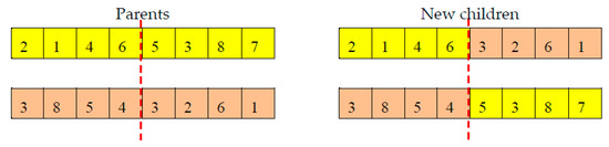
Figure 1.
One-point crossover.
Sometimes, the genetic algorithm produces very similar chromosomes. This problem is considered the symmetric problem in the genetic algorithm. Symmetric chromosomes weak the genetic algorithm and worse its performance. The symmetric problem occurs when highly fit parent chromosomes in the population breed in early evolution time. To overcome the symmetric problem, the mutation operator applied on a small part of parent chromosomes. Figure 2 illustrates the real value interchanging mutation. As shown in Figure 2, some of the genes in the chromosomes are randomly replaced. The new generation then is evaluated. New generations are still produced until the termination criterion is met, and the best-obtained chromosome is the solution [46,47]. Figure 3 proposes GA cycle to obtain the optimal solution.
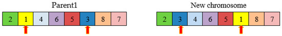
Figure 2.
Interchanging mutation.
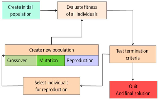
Figure 3.
Genetic algorithm cycle.
3.2. Chaos Theory for Optimization Problems
Chaos in common usage means “A condition or place of great disorder or confusion”. Chaos theory studies the behavior of systems that follow deterministic laws but appear random and unpredictable or we can say a dynamical system that has a sensitive dependence on its initial conditions; small changes in those conditions can lead to quite different outcomes [10]. This dependency of a dynamical system on its initial condition is popularly referred to as the butterfly effect. Henon initially described chaos theory in 1976 and Lorenz summarized it in 1993 [48,49]. Chaos theory could be introduced into the optimization strategy to accelerate the optimum seeking operation and find the global optimal solution. Chaos theory has an advantage more than other optimization techniques that it can efficiently search the space and escape from local optimal solutions. Chaotic maps are used to build up chaotic sequences. Different chaotic maps are proposed to describe distinct chaotic behaviors. Chaotic maps are divided to discrete-time parameterized and continuous- time parameterized. In this section, we offer some well-known chaotic maps found in the literature. Figure 4 proposes chaotic behavior produced using some chaotic maps.
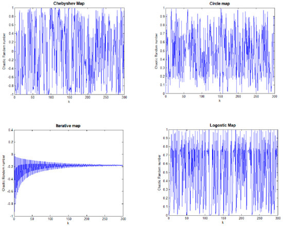
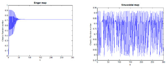
Figure 4.
Chaotic number produced using Chebyshev map, circle map, iterative map, logistic map, Singer map and Sinusoidal map.
The Chebyshev map is defined as follows:
The circle map is represented as follows:
where and .
The iterative chaotic map with infinite collapses is defined as follows:
where .
The logistic map demonstrates how complex behavior arises from a simple deterministic system without the need of any random sequence. It is based on a simple polynomial equation which describes the dynamics of biological population.
where and .
The Singer map is formulated as:
where .
The Sinusoidal map is generated by the following equation:
where .
The basic idea of applying chaos search for optimization problems is transforming problems variable to chaos space using one of the chaotic maps [47]. Followingly, chaotic variables are evaluated by the fitness function. The chaotic variables that achieve the best fitness function are the solution. Chaotic search is continued for a specified number of iterations or until obtaining a satisfied solution. Some researches compare different chaotic maps for optimization problems.
3.3. Modified Genetic Algorithm and Chaotic Search for BLPP (CGA-BS)
The proposed algorithm to solve the BLPP is a modified genetic algorithm by a new selection technique (BST) and chaos searching technique. The role of BST is that the selection of individuals for the next generation is according to individuals’ fitness to both upper and lower objective functions. BST distinguishes our proposed algorithm with a very small number of solving the lower level problem. We have solved lower level problem two times only and dispensing solving the lower level problem at every generation during solving the upper-level problem. This is not meaning that using BST replaces solving the lower level problem to have a solution of the BLPP. We solve lower level problem two times; one for the upper-level genetic algorithm based on BST solution and other for upper level chaotic local search solution. The steps of the proposed algorithm are listed as follows:
3.3.1. Genetic Algorithm Based on BST
In this Step, the upper- level problem is solved using a modified genetic algorithm. The modified genetic algorithm steps are:
- Constrains handling: before starting the algorithm, constraints of the lower level problem is added to the constraints of the upper-level problem. The feasible solutions for the upper-level problem must be feasible and optimal solutions for the lower level problem. Therefore, constrains of both levels are considered as upper level constrains to guarantee the feasibility of solutions.
- Initial population: variables are randomly initialized within the search space bounds of upper-level bounds and lower-level bounds [50].
- Reference point: the repairing process needs one feasible point considered as a reference point to be entered and the algorithm procedure is completed.
- Repairing process: for constrained problems, some generated solutions don’t satisfy constraints and need to be repaired. The repairing process transforms the infeasible solutions to be feasible solutions [51].
- Evaluation: both upper-level objective function and lower-level objective function are used for evaluation of individuals and for determining the fitness of each solution to both upper-level problem and lower-level problem.
- Producing a new population: new selection technique, crossover operator and mutation operator have applied to produce the new population.
Bilevel selection technique: The main role of BST is that the selected individuals for the next generation are more appropriate for both levels. BST starts by evaluating individuals using upper-level objective function and then are selected according to their fitness to upper-level objective function using a suitable selection technique. After that, these selected individuals are evaluated using lower-level problem objective function and are selected according to their fitness to lower-level objective function using a suitable selection technique. Bilevel selection technique can also select individuals according to upper-level objective function only or to lower-level objective function only choosing objective that increases the solution quality.
Crossover: crossover operation recombines pairs of individuals and returns the new individuals after mating two individuals. In the proposed algorithm, a one-point crossover as shown in Figure 1 which has applied [52].
Mutation: In the proposed algorithm, the real valued mutation has applied. Real valued mutation produces randomly created values and then these random values are added to the variables [53,54].
- 7.
- Migration: the parent population and child population are migrated to produce the new generation and the best individual is chosen as the solution [53,54,55].
- 8.
- GA termination: GA is terminated at the maximum number of generations or when population convergence occurs. If the termination condition doesn’t satisfy, return to 6.
3.3.2. Chaotic Local Search
In this step, a chaotic local search is proceeds around upper-level variables obtained in Section 3.3.1. The following is a description of a chaotic local search in details:
- Define a range of the upper-level variables for chaotic local search.
- Produce chaotic numbers using the logistic map: El-Shorbagy et al. in [46] presented a comparison between different chaotic maps for general nonlinear optimization problems and result that logistic map gives better performance than other chaotic maps and increase the solution quality rather than other chaotic maps. Therefore, in the proposed algorithm, we choose to apply the logistic map
- Generate the chaotic variables into the determined range.
- Find the best value: The produced chaotic variables are evaluated according to upper-level objective-function. The chaotic variables obtained best objective-function values are the best value.
- Update the local search boundary value for the best-obtained value.
- Stopping chaos search: chaotic local search is stopped at the specified iterations and put out the best solution as a local search solution.
3.3.3. Algorithm Termination
To terminate the algorithm and obtain the algorithm result, the lower level problem is solved for upper-level decision variables obtained in Section 3.3.1 and Section Section 3.3.2. The lower-level problem is solved using a genetic algorithm with the same steps as Section 3.3.2 except that selection is according to the lower level objective function only. The two phases’ results are compared, and the better result is the algorithm solution. Algorithm 1 illustrates pseudo code of the proposed algorithm. The flow chart of the proposed algorithm is shown in Figure 5.
| Algorithm 1 Modified Genetic algorithm with chaotic search for BLPP (CGA-BS) |
| 1: Modified Genetic algorithm for upper level problem 2: Begin 3: Generate an initial population with size ; 4: Check feasibility and repair out unfeasible individuals of the population ; 5: While Evaluate according to upper level objective function; Select from using selection operator; Evaluate according to lower level objective function; Select from using selection operator; Apply crossover operator with and mutation operators with on and produce children population ; |
| Evaluate the fitness of the children ; Select from using selection operator; Apply crossover operator with and mutation operators with on and produce children population ; Evaluate the fitness of the children ; Keep the best from to form Archive ; 6: End while 7: Return to the individual from with best fitness values and archive 8: Chaotic local search around modified genetic algorithm solution 9: Begin 10: While: Define range of chaotic local search Generate using different logistic ma If then and archive Else if continue, End if If termination criteria satisfied, Break End if 11: End while 12: Solve lower level problem using genetic algorithm for 13: Begin 14: Generate an initial population with size ; 15: Check feasibility and repair out unfeasible individuals of the population ; 16: While Evaluate according to lower level objective function; Select from using selection operator; Apply crossover operator with and mutation operators with on and produce children population |
| Evaluate the fitness of the children ; Keep the best from to form ; Archive ; 17: End while 18: Return to the individual from with best fitness values; 19: Evaluate the fitness of 20: Repeat from step 13 to step 18 for 21: Evaluate the fitness of 22: Return best evaluation in step 20 and 22 as algorithm solution |
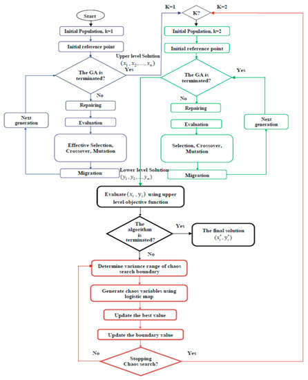
Figure 5.
The flow chart of the proposed algorithm CGA-BS.
4. Numerical Experiments
The proposed algorithm has been evaluated on three sets of well-known test problems including linear and nonlinear problems, constrained and unconstrained problems, low-dimensional and high-dimensional problems. The first set of problems is 10 constrained problems with a relatively smaller number of variables named TP problems [27]. TP problems have been extensively used test-suite for comparing different algorithms that have been solved BLPP. The second set is the SMD test set constructed in [41]. The used set of SMD problems are un-constrained high-dimensional problems that are recently proposed, which contains problems with controllable complexities. SMD test problems cover a wide range of difficulties associated with BLPP as non-linearity, multi-modality, and conflict in upper and lower level objectives. The third set is 24 nonlinear standard test problems collected from the literature [42].
For our study, the algorithm has been run 30 times for each test function. The results are median results from the runs. We use Matlab 7.8 to code the proposed algorithm CGA-BS. The simulations have been operated on an Intel Core (TM) i7-4510u CPU @2.00GHZ 2.60 GHz processor. The performance of our proposed algorithm has several parameters that affect it. The GA parameters applied on both upper and lower level problem are
- GA generation: 200–1000
- Generation gap: 0.9
- Selection operator: Stochastic universal sampling
- Crossover operator: Single point
- Mutation operator: Real-value
- Crossover rate: 0.9
- Mutation rate: 0.07
- Number of Chaotic iterations: 10,000
- Chaotic rang: 10−3
4.1. Test Problems
For our study, the algorithm has been run 30 times for each test function. The results are median results CGA-BS is tested by 40 test problems. In addition, 10 constrained test problems (TP1-TP10), 6 unconstrained high dimension test problems (SMD1-SMD6) and 24 nonlinear standard test problems collected from the literature (P1-P24). The dimension of TP problems and 24 nonlinear standard test problems is relatively small. The formulation for both TP problems and SMD problems can found at [27,41]. The formulation of standard test problems from P1 to P24 have introduced in Table A1 in Appendix A.
4.2. Results Analyses
In this section, we first compare CGA-BS results and other algorithms in the literature which solved the same chosen test set to show the effectiveness and efficiency of our algorithm. Following this, results for the TP test set have been compared with applying BST and without applying it to show how BST increases the algorithm’s performance quality. The results for the SMD test set before chaos search and after chaos search have been compared to show how chaos search increases the algorithm’s performance quality and accelerate reaching the optimal solution. In addition, proposed algorithm results and other compared algorithms results for the SMD test set have compared in terms of computational complexity to show the proposed algorithm computational time in reaching a solution.
4.2.1. TP Test Set Results Analyses
To demonstrate the effectiveness of CGA-BS, we compare CGA-BS results with results in references [27,36,42,56]. In [27] Sinha et al. presented an improved evolutionary algorithm based on quadratic approximations of lower level named it as BLEAQ. In [42], Wang et al. presented a new evolutionary algorithm based on a new constraint-handling scheme named it NEA. Wang et al. presented in [56] an evolutionary algorithm named it as NEA1. Their algorithm uses an effective crossover operator and they also propose a new mutation operator. They executed NEA1 for 50 independent runs on each of the test problems and recorded the best-obtained solutions and the worst obtained solution. To demonstrate the effectiveness of our proposed algorithm, we compare our results with the best-obtained solutions in [56]. In [36], Zhongpin et al. presented a combination between particle swarm optimization and chaos search technique PSO-CST. [36] named one of the compared results as the corresponding reference. Table 1 and Table 2 propose the values of the leader’s and the follower’s objective functions for CGA-BS and other algorithms. CGA-BS results are introduced in the second column. Third, fourth, fifth, sixth and seventh columns are the results of BLEAQ, NEA, NEA1, PSO-CST, and corresponding reference.

Table 1.
Upper level objective functions for CGA-ES, BLEAQ, NEA, NEA1, PSO-CST and BLEAQ and corresponding reference [36] in algorithms for TP1-TP10.
Table 2.
Lower level objective functions by CGA-ES, BLEAQ, NEA, NEA1, PSO-CST and BLEAQ and corresponding reference [36] algorithms for TP1-TP10.
Solving BLPP is executed by solving the lower level problem as a constraint to the upper-level problem. The main aim is to solve the upper-level problem. Therefore, in a comparison between CGA-BS and other algorithms, we are concerned about upper-level results. As Table 1 indicates, our proposed algorithm has the best results for the upper-level problem than other algorithms for six problems TP1, TP2, TP3, TP4, TP6, and TP9. The remainder of problems have also a small difference with the best solutions of compared algorithms. Figure 6 shows the difference between the upper-level objective-function result and the best upper-level objective-function result of the compared algorithms results for TP test problems. This difference is denoted by upper-level accuracy. From Figure 6, the proposed algorithm has the smallest upper-level accuracy which means that the proposed algorithm more converges to the optimal solution. We rank the different algorithms according to the best upper-level solution for all algorithms in Table A2 (see Appendix B). Figure 7 illustrates the ranks obtained with CGA-BS and other algorithms. From the tables and figures, the CGA-BS algorithm obtained the first rank for six problems and reach to the second rank for four problems. From results, we can consider CGA-BS performs well and finds good solutions to TP test problems.

Figure 6.
Upper-level accuracy obtained with CGA-ES and three well-known algorithms for TP test problems.

Figure 7.
Ranks obtained with CGA-BS and five well-known algorithms for TP test problems.
4.2.2. SMD Test Set Results Analyses
The results of SMD test problems are presented in Table 3. The second column presents the optimal solution for the upper level and lower-level problems. CGA-BS results for upper level and lower level problems are in the third columns. As indicated in Table 3, our proposed algorithm reaches optimal solutions for two problems SMD1, SMD3 and reaches near to optimal solutions for the remaining problems. To evaluate the CGA-BS algorithm for SMD problems, we compare CGA-BS results with the other four algorithms listed in [57] and three algorithms listed in [58]. Table 4 illustrates a comparison between CGA-BS and other algorithms. We have been compared algorithms with CGA-BS according to upper-level accuracy. Accuracy is the difference between the algorithm result and an optimal solution. Figure 8 illustrates the upper-level accuracy for compared results. From Figure 8, that proposed algorithm more converges to the optimal solution than other compared algorithms for SMD test problems. In addition, we rank the different algorithms and CGA-ES algorithm in Table A3 (see Appendix B). Figure 9 illustrates the ranks obtained with CGA-BS and other algorithms. From the tables and figures, the CGA-BS algorithm obtained the first rank for four problems from six problems. CGA-BS performs well for SMD test and more convergence to the optimal solution concerning to compared algorithms. It can be concluded that CGA-BS can manage the difficulties resulting from the increasing problem dimension. In addition, results show that algorithm FOA also performs well and more convergence to the optimal solution. FOA treat BLPP by combining two improved fruit fly optimization algorithms. Fruit fly algorithm is one of the powerful evolutionary algorithms. It has a huge advantage in that it has a very small control parameter. The results illustrated that CGA-BS and FOA algorithms is an effective technique to solve a large dimension BLPP.
Table 3.
CGA-BS results and optimal solutions for SMD1–SMD6.
Table 4.
CGA-BS, BLMA, NBLEA, BLEAQ, BIDE, FOA, PSO, LGMS-FOA upper level accuracy for SMD1–SMD6.
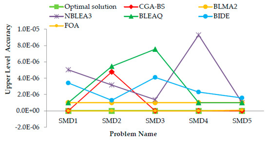
Figure 8.
Upper-level accuracy obtained with CGA-ES and five well-known algorithms for SMD1–SMD5 test problems.

Figure 9.
Ranks obtained with CGA-BS and five well-known algorithms for SMD test problem.
4.2.3. P1–P24 Test Set Results Analyses
Table 5 presents CGA-BS results for P1–P24 problems and the best-obtained solution of the upper level and lower level objective functions in references [36,56]. In Table 6, CGA-BS find solutions better than best-obtained solutions in [36] for all problems solved in it except P17. It can be considered that CGA-BS has superiority over the algorithm PSO-CST algorithm. Figure 10 illustrates the upper-level accuracy for CGA-BS, NEA1 and PSO-CST algorithms. It can be observed from Figure 10 that CGA-BS more converges to the optimal solution. Ranks CGA-ES, NEA1 algorithm in Table A4 (see Appendix B). Figure 11 illustrates the ranks obtained with CGA-BS and other algorithms. CGA-BS find solutions better than a best-obtained solution in [56] for eleven problems and reach to same upper-level solutions in [56] three problems from twenty-one problems has solved in [56]. CGA-ES obtained the first rank for fourteen problems from the twenty-one problem. It can be considered that CGA-BS performs well than the algorithm in [36,56] for P1–P24.
Table 5.
CGA-BS results and best obtained solutions in [35] for P1–P24.
Table 6.
The proposed algorithm results with and without bi-level selection technique.
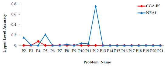
Figure 10.
Upper-level accuracy obtained with CGA-ES, NEA1 algorithms for P1–P21.
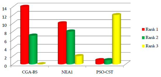
Figure 11.
Ranks obtained with CGA-BS, NEA1, and PSO-CST algorithms for P1–P24.
The proposed algorithm has evaluated 40 test problems. A total of 37 test problems weere solved with other algorithms. Our proposed algorithm obtained the best solutions compared to the mentioned references for nineteen problems and reach to same best solutions for five problems. The difference between our results and the best solutions for remaining problems ranges from 1E-1 to 1E-12 except for P4 and P8. Figure 12 indicates the difference between CGA-BS and best-compared solutions in the mentioned references for the upper-level results. The negative difference indicates to CGA-BS has better solutions than best-compared solutions. Figure 13 presents the statistics of the ranks of CGA-BS. Statistics of ranking in Table A5 (see Appendix B). Figure 14 presents the rank’s percentage for the proposed algorithm. As indicated in Figure 14, our proposed algorithm obtained first rank for about 65% of solved problems and obtained second rank for about 32.5% of solved problems.
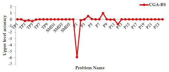
Figure 12.
Upper level accuracy for all solved problems.
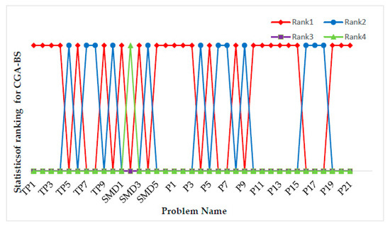
Figure 13.
Statistics of ranking obtained by the proposed algorithm (CGA-BS) for test problems.

Figure 14.
Rank’s percentages of the proposed algorithm (CGA-BS) for test problems.
The simulations results of various numerical studies have been demonstrated that CGA-BS effectively solves BLPP and it can manage the difficulties resulting from increasing dimension of the problem. In addition, results have been demonstrated the superiority of CGA-BS on compared algorithms solved the same test problems.
4.2.4. Algorithm Performance Analyses with Bilevel Selection Technique
The basic idea of the bi-level selection technique is selecting more appropriate solutions that can increase the solution quality. The individuals are selected for producing the new generation during solving upper-level problem according to both the upper and lower level. Table 6 illustrates the algorithm results for TP test problems with applying the bilevel selection technique (CGA-BS) and without applying it (CGA). Figure 15 illustrates the upper-level accuracy for TP set with and without the bilevel selection technique. The results illustrate that using an effective selection technique improve the solution quality for TP1, TP5, and TP6. We note from results BST does not improve results for all problems. That is due to the conflict between upper and lower level objectives. As a result, applying an effective selection technique enables the algorithm to increase its performance quality and accelerate reaching the optimal solution especially for not conflicted upper and lower objective functions.
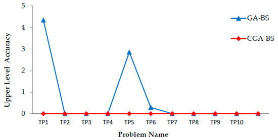
Figure 15.
Upper-level accuracy obtained by the proposed algorithm with and without algorithms bilevel selection technique for Tp1–Tp10.
4.2.5. Algorithm Performance Analyses with Chaos Search
To analyze our proposed algorithm performance, a comparison between algorithm results before chaos search (GA-BS) and after applying (CGA-BS). Table 7 illustrates algorithm results for SMD test set before applying chaos search and after applying it for both upper level and lower level problem. As illustrated in Table 7, the results after applying chaos search more converges to optimal solutions. Figure 16 illustrate the upper level accuracy for SMD set before applying chaos search and after applying it. The results reveal that applying chaos search helps to more converges to optimal solutions and the integrating between genetic algorithm and a chaos search accelerates the optimum seeking operation and helps to more converges to optimal solutions.
Table 7.
GA-BS and CGA-BS results for SMD1–SMD6.
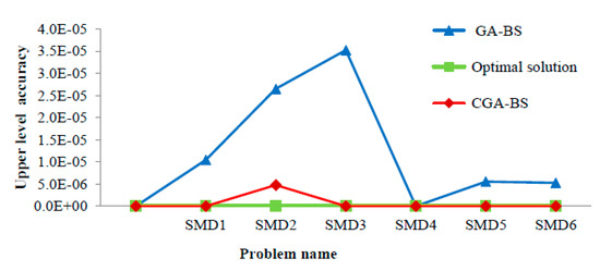
Figure 16.
Upper level accuracy for GA-BS and CGA-BS for SMD1–SMD6.
4.2.6. Computational Expense
In BLPP, the feasible space is very large. BLPP consists of two nested optimization problem. The upper-level problem feasible space is the optimal solution of lower-level problem. With another meaning, finding one feasible solution of the upper-level problem requires solving lower-level problem. This huge feasible space makes the computational complexity for BLPP is NP. To evaluate the computational complexity of BLPP, number of function evaluations is used as a measure of the computational time. CGA-BS functions evaluations and other algorithms function evaluations for SMD test set are compared to show proposed algorithm speed convergence to reach to the optimal solution. The upper-level function evaluations of proposed algorithm and BLMA, NBLE, BLEAQ, BIDE algorithms in [57] set are presented in Table 8. The lower-level function evaluations of proposed algorithm and BLMA, NBLE, BLEAQ, BIDE algorithms in [57] are presented in Table 9. The total function evaluations for both upper-level and lower-level of proposed algorithm and other compared algorithms are presented in Table 10. Figure 17 proposed the total function evaluations of proposed algorithm and compared algorithm. As illustrated, proposed algorithm needs a smaller number of total function evaluation than compared algorithms for three problems. In addition, the compared algorithms and CGA-ES algorithm are ranked according to total function evaluations in Table A6 (see Appendix B). Figure 18 illustrates the ranks percentage obtained with CGA-BS. CGA-BS reaches to first rank for fifty percent of SMD test problems with compared algorithms. From results, the proposed algorithm reaches to the best results in a much shorter time. It can be considered as an effective and comparable algorithm for BLPP.
Table 8.
Median upper level function evaluations for CGA-BS and four known algorithms for SMD test problem.
Table 9.
Median Lower level function evaluations for CGA-BS and four known algorithms for SMD test problem.
Table 10.
Median total function evaluations for CGA-BS and four known algorithms for SMD test problem.
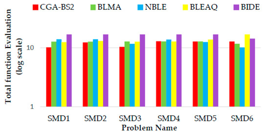
Figure 17.
Median total function evaluations for CGA-BS and four known algorithms for SMD test problem.
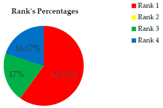
Figure 18.
Rank percentages of the proposed algorithm according total function evaluations for SMD test problems.
5. Conclusions
This paper proposed a genetic algorithm supported by new selection technique and chaos theory to solve bilevel programming problems. The combination between genetic algorithm and chaos search offer the advantages of both genetic algorithm as a powerful global searching technique and chaos search as an efficient and fast searching technique. The new effective selection technique increases algorithm performance quality and accelerate reaching to the optimal solution. Extensive numerical experiments for multimodal test functions including ten constrained problems with relatively smaller number of variables, six unconstrained high-dimensional problems and twenty-four nonlinear standard test problems are performed to verify the performance of CGA-BS. The CGA-BS results have analyzed and compared with other state-of-the-art algorithms to show demonstration and efficiency of our proposed algorithm. A careful observation of proposed algorithm results and other state-of-the-art results will reveal to the following benefits:
CGA-BS can be considered as a global powerful efficient technique to solve BLPP and can treat with the difficulties associated with BLPP as non-linearity, multi-modality and confliction between the upper and lower level objectives.
CGA-BS deals with several sets of problems including linear and nonlinear problems, constrained and unconstrained problems, low-dimensional and high-dimensional problems.
CGA-BS has better ability and precision than other proposed methods in literature and was demonstrated to be extremely efficient at locating optimal solutions.
The new selection technique helps the upper level decision maker to choose a solution appropriated to lower level problem and more convergence to the optimal solution by dispensing solving lower level problem for every generation during solving upper level problem.
The new effective selection technique enables the algorithm to increase its performance quality and accelerate reaching to the optimal solution.
The search using chaos theory enhances the search characteristics, helps in faster convergence of the algorithm.
CGA-BS not only reaches to good solution for BLPP. It can reach to it with acceptable running time.
In our future works, the following will be researched:
- (a)
- Adapting CGA-BS to solve multi-level programming problems
- (b)
- Updating CGA-BS to solve the multi-objective multi-level programming problems.
Author Contributions
Conceptualization, Y.A.-E. and S.N.; methodology Y.A.-E. and S.N.; software, Y.A.-E. and S.N.; validation, Y.A.-E. and S.N.; formal analysis, Y.A.-E. and S.N.; investigation, Y.A.-E. and S.N.; resources, Y.A.-E. and S.N.; data curation, Y.A.-E. and S.N.; writing—original draft preparation, Y.A.-E., S.N.; writing—review and editing, Y.A.-E. and S.N.; visualization, Y.A.-E. and S.N.; supervision, Y.A.-E.; project administration, Y.A.-E.; All authors have read and agreed to the published version of the manuscript.
Funding
This research received no external funding.
Conflicts of Interest
The authors declare no conflicts of interest.
Abbreviation
: Upper level Population size, : Lower level Population size,: Number of upper level generations, : Number of Lower level generations, : Crossover probability, : mutation probability, selection operator, crossover and mutation operators, : Chaotic size, Number of Chaotic iterations, : Chaotic range.
Appendix A
Table A1 proposes a formulation of standard test problem from P1 to P24. Problem dimensions is denoted by (n, m). Dimensions (n) denotes to the upper level dimensions. Dimensions (m) denotes to the lower level dimensions.
Table A1.
BLPP formulation for problems P1–P24.
Table A1.
BLPP formulation for problems P1–P24.
| Problem Formulation (n, m) | Problem Formulation (n, m) |
|---|---|
| P1 | P2 |
| P3 | P4 |
| P5 | P6 |
| P7 | P8 |
| P9 | P10 |
| P11 | P12 |
| P13 | P14 |
| P15 | P16 |
| P17 | P18 |
| P19 | P20 |
| P21 | P22 |
| P23 | P24 |
Appendix B
Table A2.
Ranks for CGA-BS, BLEAQ, NEA, NEA1, PSO-CST and BLEAQ and the corresponding reference in [36] according to upper level objective functions for TP1–TP10.
Table A2.
Ranks for CGA-BS, BLEAQ, NEA, NEA1, PSO-CST and BLEAQ and the corresponding reference in [36] according to upper level objective functions for TP1–TP10.
| Problem | Rank According to Upper Level | |||||
|---|---|---|---|---|---|---|
| CGA-BS | BLEAQ [27] | NEA [41] | NEA1 [56] | PSO-CST [36] | Cor. Ref. [36] | |
| TP1 | Rank1 | Rank1 | Rank1 | Rank1 | - | Rank1 |
| TP2 | Rank1 | Rank2 | Rank1 | Rank1 | - | Rank3 |
| TP3 | Rank1 | Rank2 | Rank4 | Rank4 | Rank3 | Rank4 |
| TP4 | Rank1 | Rank4 | Rank3 | Rank3 | Rank2 | Rank3 |
| TP5 | Rank2 | Rank3 | Rank1 | Rank1 | - | Rank4 |
| TP6 | Rank1 | Rank2 | Rank2 | Rank2 | Rank3 | Rank4 |
| TP7 | Rank2 | Rank3 | Rank1 | Rank1 | Rank1 | Rank1 |
| TP8 | Rank2 | Rank3 | Rank1 | Rank1 | - | Rank3 |
| TP9 | Rank1 | Rank2 | - | - | - | - |
| TP10 | Rank2 | Rank1 | - | - | - | - |
Table A3.
Ranks for CGA-BS, BLMA, NBLEA, BLEAQ, BIDE, FOA, PSO, LGMS-FOA algorithms according to upper level accuracy for SMD1–SMD6.
Table A3.
Ranks for CGA-BS, BLMA, NBLEA, BLEAQ, BIDE, FOA, PSO, LGMS-FOA algorithms according to upper level accuracy for SMD1–SMD6.
| Problem | Rank According to Upper Level | |||||||
|---|---|---|---|---|---|---|---|---|
| CGA-BS | BLMA [57] | NBLEA [57] | BLEAQ [57] | BIDE [57] | FOA [58] | PSO [58] | LGMS-FOA [58] | |
| SMD1 | Rank 1 | Rank 3 | Rank 5 | Rank 3 | Rank 4 | Rank 2 | Rank7 | Rank 6 |
| SMD2 | Rank 4 | Rank2 | Rank 5 | Rank 6 | Rank 3 | Rank 1 | Rank 8 | Rank7 |
| SMD3 | Rank 1 | Rank 3 | Rank 4 | Rank 6 | Rank 5 | Rank 2 | Rank 8 | Rank 7 |
| SMD4 | Rank 2 | Rank 3 | Rank 5 | Rank 3 | Rank 4 | Rank 1 | Rank 7 | Rank 6 |
| SMD5 | Rank 1 | Rank 3 | Rank 3 | Rank 3 | Rank 4 | Rank 2 | Rank 6 | Rank 5 |
| SMD6 | Rank 1 | Rank 2 | Rank 2 | Rank 2 | Rank 3 | - | - | - |
Table A4.
Ranks for CGA-BS, NEA1, PSO-CST algorithms according to upper level accuracy for SMD1–SMD6.
Table A4.
Ranks for CGA-BS, NEA1, PSO-CST algorithms according to upper level accuracy for SMD1–SMD6.
| Problem | Rank According to Upper Level | ||
|---|---|---|---|
| CGA-BS | NEA1 [56] | PSO-CST [36] | |
| P1 | Rank1 | Rank2 | Rank3 |
| P2 | Rank1 | Rank2 | Rank3 |
| P3 | Rank1 | Rank2 | - |
| P4 | Rank2 | Rank1 | - |
| P5 | Rank1 | Rank2 | - |
| P6 | Rank2 | Rank1 | - |
| P7 | Rank2 | Rank1 | - |
| P8 | Rank1 | Rank2 | Rank3 |
| P9 | Rank2 | Rank1 | Rank3 |
| P10 | Rank1 | Rank2 | Rank3 |
| P11 | Rank1 | Rank3 | Rank2 |
| P12 | Rank1 | Rank2 | - |
| P13 | Rank1 | Rank1 | - |
| P14 | Rank1 | Rank1 | Rank2 |
| P15 | Rank1 | Rank1 | Rank2 |
| P16 | Rank2 | Rank1 | Rank3 |
| P17 | Rank2 | Rank3 | Rank1 |
| P18 | Rank2 | Rank1 | Rank3 |
| P19 | Rank1 | Rank2 | Rank3 |
| P20 | Rank1 | Rank2 | Rank3 |
| P21 | Rank1 | Rank2 | Rank3 |
Table A5.
Statistics of ranks of CGA-BS for TP1–TP10, SMD1–SMD6, and P1–P21.
Table A5.
Statistics of ranks of CGA-BS for TP1–TP10, SMD1–SMD6, and P1–P21.
| Problem | Statistics of Ranks | |||
|---|---|---|---|---|
| Rank1 | Rank2 | Rank3 | Rank4 | |
| TP1 | 1 | 0 | 0 | 0 |
| TP2 | 1 | 0 | 0 | 0 |
| TP3 | 1 | 0 | 0 | 0 |
| TP4 | 1 | 0 | 0 | 0 |
| TP5 | 0 | 1 | 0 | 0 |
| TP6 | 1 | 0 | 0 | 0 |
| TP7 | 0 | 1 | 0 | 0 |
| TP8 | 0 | 1 | 0 | 0 |
| TP9 | 1 | 0 | 0 | 0 |
| TP10 | 0 | 1 | 0 | 0 |
| SMD1 | 1 | 0 | 0 | 0 |
| SMD2 | 0 | 0 | 0 | 1 |
| SMD3 | 1 | 0 | 0 | 0 |
| SMD4 | 0 | 1 | 0 | 0 |
| SMD5 | 1 | 0 | 0 | 0 |
| SMD6 | 1 | 0 | 0 | 0 |
| P1 | 1 | 0 | 0 | 0 |
| P2 | 1 | 0 | 0 | 0 |
| P3 | 1 | 0 | 0 | 0 |
| P4 | 0 | 1 | 0 | 0 |
| P5 | 1 | 0 | 0 | 0 |
| P6 | 0 | 1 | 0 | 0 |
| P7 | 0 | 1 | 0 | 0 |
| P8 | 1 | 0 | 0 | 0 |
| P9 | 0 | 1 | 0 | 0 |
| P10 | 1 | 0 | 0 | 0 |
| P11 | 1 | 0 | 0 | 0 |
| P12 | 1 | 0 | 0 | 0 |
| P13 | 1 | 0 | 0 | 0 |
| P14 | 1 | 0 | 0 | 0 |
| P15 | 1 | 0 | 0 | 0 |
| P16 | 0 | 1 | 0 | 0 |
| P17 | 0 | 1 | 0 | 0 |
| P18 | 0 | 1 | 0 | 0 |
| P19 | 1 | 0 | 0 | 0 |
| P20 | 1 | 0 | 0 | 0 |
| P21 | 1 | 0 | 0 | 0 |
Table A6.
Ranks for CGA-BS, BLMA, NBLEA, BLEAQ, BIDE algorithms according to total function evaluations for SMD1–SMD6.
Table A6.
Ranks for CGA-BS, BLMA, NBLEA, BLEAQ, BIDE algorithms according to total function evaluations for SMD1–SMD6.
| Problem | Rank According to Total of Function Evaluations | ||||
|---|---|---|---|---|---|
| CGA-BS | BLMA [57] | NBLEA [57] | BLEAQ [57] | BIDE [57] | |
| SMD1 | Rank 1 | Rank 3 | Rank 4 | Rank 2 | Rank 5 |
| SMD2 | Rank 1 | Rank2 | Rank 4 | Rank 3 | Rank 5 |
| SMD3 | Rank 1 | Rank 3 | Rank 4 | Rank 2 | Rank 5 |
| SMD4 | Rank 3 | Rank 2 | Rank 4 | Rank 1 | Rank 5 |
| SMD5 | Rank 1 | Rank 2 | Rank 4 | Rank 3 | Rank 5 |
| SMD6 | Rank 4 | Rank 3 | Rank 2 | Rank 1 | Rank 5 |
References
- Kalashnikov, V.; Dempe, S.; Pérez-Valdés, A.; Kalashnykova, I.; Camacho-Vallejo, J. Bilevel programming and applications. Math. Probl. Eng. 2015, 2015, 1–16. [Google Scholar] [CrossRef]
- Ruusk, S.; Miettinen, K.; Wiecek, M. Connections between single-level and bilevel multiobjective optimization. J. Optimiz. Theory App. 2012, 153, 60–74. [Google Scholar] [CrossRef][Green Version]
- Shuang, M. A nonlinear bi-level programming approach for product portfolio management. SpringerPlus 2016, 5, 1–18. [Google Scholar]
- Gaspar, I.; Benavente, J.; Bordagaray, M.; Alonso, B.; Moura, J.L.; Ibeas, Á. A bilevel mathematical programming model to optimize the design of cycle paths. Transp. Res. Procedia 2015, 10, 423–443. [Google Scholar] [CrossRef]
- Aihong, R.; Yuping, W.; Xingsi, X. A novel approach based on preference-based index for interval bilevel linear programming problem. J. Inequal. Appl. 2017, 2017, 1–16. [Google Scholar]
- Birla, R.; Agarwal, V.; Khan, I.; Mishra, V. An alternative approach for solving bilevel programming problems. Am. J. Oper. Res. 2017, 7, 239–247. [Google Scholar]
- Osman, M.; Emam, M.; Elsayed, M. Interactive approach for multi-level multi-objective fractional programming problems with fuzzy parameters. J. Basic Appl. Sci. 2018, 7, 139–149. [Google Scholar] [CrossRef]
- Dempe, S.B. Bilevel Optimization: Theory, Algorithms and Applications; Fakultät für Mathematik und Informatik: Freiberg, Germany, 2018. [Google Scholar]
- Borowska, B.B. Social Strategy of Particles in Optimization Problems; Springer: Cham, Switzerland, 2020; pp. 537–546. [Google Scholar]
- Zhan, Y.; Zheng, Q. A multistage decision-dependent stochastic bilevel programming approach for power generation investment expansion 525 planning. IISE Trans. 2018, 50, 720–734. [Google Scholar] [CrossRef]
- Migdalas, A.; Pardalos, M.; Värbrand, P. Multilevel Optimization: Algorithms and Applications; Springer Science & Business Media: Berlin, Germany, 2013. [Google Scholar]
- Jie, L.; Jialin, H.; Yaoguang, H.; Guangquan, Z. Multilevel decision-making: A survey. Inf. Sci. 2016, 346, 463–487. [Google Scholar]
- Wang, G.; Wan, Z.; Wang, X.; Yibing, L. Genetic algorithm based on simplex method for solving linear-quadratic bilevel programming problem. Comput. Math. Appl. 2008, 56, 2550–2555. [Google Scholar] [CrossRef]
- El-Desoky, I.; El-Shorbagy, M.; Nasr, S.; Hendawy, Z.; Mousa, A. A Hybrid Genetic Algorithm for Job Shop Scheduling Problem. Int. J. Adv. Eng. Technol. Comput. Sci. 2016, 3, 6–17. [Google Scholar]
- Hosseini, E. Solving linear tri-level programming problem using heuristic method based on bi-section algorithm. Asian J. Sci. Res. 2017, 10, 227–235. [Google Scholar] [CrossRef]
- Dempe, S.; Kue, F. Solving discrete linear bilevel optimization problems using the optimal value reformulation. Glob. Optim. 2017, 68, 255–277. [Google Scholar] [CrossRef]
- Zhenyuan, L.; Zaisheng, L.; Zhipeng, Z.; Shen, Y.; Dong, J. Simulated annealing for a multi-level nurse rostering problem in hemodialysis service. Appl. Soft Comput. 2017, 64, 148–160. [Google Scholar]
- Jialin, H.; Guangquan, Z.; Yaoguang, H.; Jie, L. Solving tri-level programming problems using a particle swarm optimization algorithm. In Proceedings of the Conference on Industrial Electronics and Applications, Auckland, New Zealand, 15–17 June 2015. [Google Scholar]
- Lachhwani, K.; Dwivedi, A.; Goyal, D. Feasibility of lingo software for bi-Level programming problems (BLPPs): A study. In Proceedings of the Sixth International Conference on Soft Computing for Problem Solving, Patiala, India, 23–24 December 2016. [Google Scholar]
- Yabo, L.; Yongo, P. The improved ant colony optimization algorithm for mlp considering the advantage from relationship. Math. Probl. Eng. 2017, 2017, 1–11. [Google Scholar]
- Khan, S.; Baig, A. Ant colony optimization based hierarchical multi-label classification algorithm. Appl. Soft Comput. 2017, 55, 462–479. [Google Scholar] [CrossRef]
- Shiha, H.; Wen, U.; Lee, S.; Lan, K.; Hsiao, H. A neural network approach to multiobjective and multilevel programming problems. Comput. Math. Appl. 2004, 48, 95–108. [Google Scholar] [CrossRef]
- Sinha, A.; Malo, P.; Deb, K. A Review on bilevel optimization: From classical to evolutionary approaches and applications. IEEE Trans. Evolut. Comput. 2017, 22, 276–295. [Google Scholar] [CrossRef]
- Zhang, T.; Chen, Z.; June, L.; Xiong, L. The artificial neural networks based on scalarization method for a class of bilevel biobjective programming problem. Comput. Intell. Neurosci. 2017, 2017, 1–14. [Google Scholar] [CrossRef]
- Bard, J.; Moore, J. A branch and bound algorithm for the bilevel programming problem. Siam J. Sci. Stat. Comp. 1990, 11, 281–292. [Google Scholar] [CrossRef]
- Sinha, A.; Malo, P.; Deb, K. An improved bilevel evolutionary algorithm based on quadratic approximations. In Proceedings of the 2014 IEEE Congress on Evolutionary Computation, Beijing, China, 6–11 July 2014. [Google Scholar]
- Sinha, A.; Malo, P.; Deb, K. Evolutionary algorithm for bilevel optimization using approximations of the lower level optimal solution mapping. Eur. J. Oper. Res. 2016, 275, 395–411. [Google Scholar] [CrossRef]
- Sinha, A.; Lu, Z.; Deb, K.; Malo, P. Bilevel optimization based on iterative approximation of multiple mappings. J. Heuristics 2020, 26, 151–185. [Google Scholar] [CrossRef]
- Carrasqueira, P.; Alves, M.; Antunes, C. Bi-level particle swarm optimization and evolutionary algorithm approaches for residential demand response with different user profiles. Inf. Sci. 2017, 418, 405–420. [Google Scholar] [CrossRef]
- Lan, K.; Wen, U.; Shih, H.; Stanley Lee, E. A hybrid neural network approach to bilevel programming problems. Appl. Math. Lett. 2007, 20, 880–884. [Google Scholar] [CrossRef]
- Anter, A.; Ali, M. Feature selection strategy based on hybrid crow search optimization algorithm integrated with chaos theory and fuzzy c-means algorithm for medical diagnosis problems. Soft Comput. 2020, 24, 1565–1584. [Google Scholar] [CrossRef]
- Jampour, M. Chaotic genetic algorithm based on lorenz chaotic system for optimization problems. Intell. Syst. Appl. 2013, 5, 19–24. [Google Scholar]
- Liu, B.; Wang, L.; Jin, Y.; Tang, F.; Huang, D. Improved particle swarm optimization combined with chaos. Chaos Solitons Fract. 2005, 25, 1261–1271. [Google Scholar] [CrossRef]
- Xiang, T.; Liao, X.; Wong, K. An improved particle swarm optimization algorithm combined with piecewise linear chaotic map. Appl. Math. Comput. 2007, 190, 1637–1645. [Google Scholar] [CrossRef]
- Gue, S.; Wang, J.; Ma, X. Improved Bat Algorithm Based on Multipopulation Strategy of Island Model for Solving Global Function Optimization Problem. Comput. Intell. Neurosc. 2019, 2019, 1–12. [Google Scholar] [CrossRef]
- Alatas, B.; Akin, E.; Ozer, A. Chaos embedded particle swarm optimization algorithms. Chaos Soliton Fract. 2009, 40, 1715–1734. [Google Scholar] [CrossRef]
- Yousria, A.; Nasr, S.; El-Desoky, I.; Hendawy, Z.; Mousa, A. Enhanced Genetic Algorithm and Chaos Search for Bilevel Programming Problems. In Advances in Intelligent Systems and Computing; Hassanien, A., Ed.; Springer: Cham, Switzerland, 2019; pp. 478–487. [Google Scholar]
- Zhongping, W.; Guangmin, W.; Bin, S. A hybrid intelligent algorithm by combining particle swarm optimization with chaos searching technique for solving nonlinear bilevel programming problems. Swarm Evol. Comput. 2013, 8, 26–32. [Google Scholar]
- Zhao, H.; Gao, Z. Chaos Search Method for Bilevl Programming. J. Syst. Sci. Inf. 2005, 3, 553–560. [Google Scholar]
- Sinha, A.; Malo, P.; Kalyanmoy, D. Test problem construction for single-objective bilevel optimization. Evol. Comput. 2014, 22, 439–477. [Google Scholar] [CrossRef] [PubMed]
- Sinha, A.; Malo, P.; Deb, K. Unconstrained scalable test problems for Single-objective bilevel optimization. In Proceedings of the 2012 IEEE Congress on Evolutionary Computation, Brisbane, QLD, Australia, 10–15 June 2012. [Google Scholar]
- Wang, Y.; Jiao, Y.; Li, H. An evolutionary algorithm for solving nonlinear bilevel programming based on a new constraint-handling scheme. IEEE Transp. Syst. Man Cybern. Part C 2005, 35, 221–232. [Google Scholar] [CrossRef]
- Colson, B.; Marcotte, P.; Savard, G. An overview of bilevel optimization. Ann. Oper. Res. 2007, 153, 235–256. [Google Scholar] [CrossRef]
- Nasr, S.; El-Shorbagy, M.; El-Desoky, I.; Hendawy, Z.; Mousa, A. Hybrid genetic algorithm for constrained nonlinear optimization problems. Brit. J. Math. Comput. Sci. 2015, 7, 466–480. [Google Scholar] [CrossRef]
- Abd-El-Wahed, W.; Mousa, A.; El-Shorbagy, M. Integrating particle swarm optimization with genetic algorithms for solving nonlinear optimization problems. J. Comput. Appl. Math. 2011, 235, 1446–1453. [Google Scholar] [CrossRef]
- El-Shorbagy, M.; Mousa, A.; Nasr, S. A chaos-based evolutionary algorithm for general nonlinear programming problems. Chaos Soliton Fract. 2016, 85, 8–21. [Google Scholar] [CrossRef]
- Tavazoei, M.; Haeri, M. Comparison of different one-dimensional maps as chaotic search pattern in chaos optimization algorithms. Appl. Math. Comput. 2007, 187, 76–85. [Google Scholar] [CrossRef]
- Hilborn, R.B. Chaos and Nonlinear Dynamics: An Introduction for Scientists and Engineers, 2nd ed.; Oxford University Press: Oxford, UK, 2004. [Google Scholar]
- Lu, P.; Zhou, J.; Zhang, H.; Zhang, R.; Wang, C. Chaotic differential bee colony optimization algorithm for dynamic economic dispatch problem with valve-point effects. Int. J. Electr. Power 2014, 62, 130–143. [Google Scholar] [CrossRef]
- Mousa, A.; El-Shorbagy, M.; Abd-El-Wahed, W. Local search-based hybrid particle swarm optimization algorithm for multiobjective optimization. Swarm Evol. Comput. 2012, 3, 1–14. [Google Scholar] [CrossRef]
- Mousa, A.A.; El-Wahed, W.F.A.; Rizk-Allah, R.M. A hybrid ant optimization approach based local search scheme for multiobjective design optimizations. Electr. Power Syst. Res. 2011, 81, 1014–1023. [Google Scholar] [CrossRef]
- Mousa, A. Hybrid ant optimization system for multiobjective economic emission load dispatch problem under fuzziness. Swarm Evol. Comput. 2014, 81, 11–21. [Google Scholar] [CrossRef]
- Genlin, J. Survey on genetic algorithm. Comput. Appl. Soft 2004, 2, 69–73. [Google Scholar]
- Osman, M.; Abo-Sinna, M.; Mousa, A. A solution to the optimal power flow using genetic algorithm. Appl. Math. Comput. 2004, 155, 391–405. [Google Scholar] [CrossRef]
- Mirjalili, S.; Dong, J.; Sadiq, A.; Faris, H.B. Genetic Algorithm: Theory, Literature Review, and Application in Image Reconstruction. In Studies in Computational Intelligence; Springer: Cham, Switzerland, 2019; pp. 69–85. [Google Scholar]
- Wang, Y.; Li, H.; Dang, C. A new evolutionary algorithm for a class of nonlinear bilevel programming problems and its global convergence. Inf. J. Comput. 2011, 23, 618–629. [Google Scholar] [CrossRef]
- Islam, M.; Singh, H.; Ray, T.; Sinha, A. An enhanced memetic algorithm for single-objective bilevel optimization problem. Evol. Comput. 2016, 25, 607–642. [Google Scholar] [CrossRef]
- Wang, G.; Ma, L.; Chen, J. A bilevel improved fruit fly optimization algorithm for the nonlinear bilevel programming problem. Knowl.-Based Syst. 2017, 138, 113–123. [Google Scholar] [CrossRef]
© 2020 by the authors. Licensee MDPI, Basel, Switzerland. This article is an open access article distributed under the terms and conditions of the Creative Commons Attribution (CC BY) license (http://creativecommons.org/licenses/by/4.0/).