Image Zooming Based on Two Classes of C¹-Continuous Coons Patches Construction with Shape Parameters over Triangular Domain

Abstract

Image interpolation is important in image zooming. To improve the quality of image zooming, in this work, we proposed a class of rational quadratic trigonometric Hermite functions with two shape parameters and two classes of $C^1$-continuous Coons patches constructions over a triangular domain by improved side–side method and side–vertex method. Altering the values of shape parameters can adjust the interior shape of the triangular Coons patch without influencing the function values and partial derivatives of the boundaries. In order to deal with the problem of well-posedness in image zooming, we discussed symmetrical sufficient conditions for region control of shape parameters in the improved side–side method and side–vertex method. Some examples demonstrate the proposed methods are effective in surface design and digital image zooming. $C^1$-continuous Coons patches constructed by the proposed methods can interpolate to scattered 3D data. By up-sampling to the constructed interpolation surface, high-resolution images can be obtained. Image zooming experiment and analysis show that compared to bilinear, bicubic, iterative curvature-based interpolation (ICBI), novel edge orientation adaptive interpolation scheme for resolution enhancement of still images (NEDI), super-resolution using iterative Wiener filter based on nonlocal means (SR-NLM) and rational ball cubic B-spline (RBC), the proposed method can improve peak signal to noise ratio (PSNR) and structural similarity index (SSIM). Edge detection using Prewitt operator shows that the proposed method can better preserve sharp edges and textures in image zooming. The proposed methods can also improve the visual effect of the image, therefore it is efficient in computation for image zooming.

1. Introduction

Image zooming refers to constructing a high resolution (HR) image from a low resolution (LR) image, which is to estimate unknown pixels from known pixels in essence. Image interpolation technology can preserve rich texture information and sharp edges under certain conditions. Image interpolation technology plays an important role in the field of image processing and is widely used in various fields, such as aerospace, military, communications, remote sensing satellites, television and film production.

The earliest interpolation methods consist of nearest-neighbor interpolation, bilinear interpolation [1], bicubic interpolation [2,3] and so on. These methods work well in smooth areas, with obvious alias and ringing in edge texture areas. Lehmann et al. [4] discussed the image magnification method based on B-spline interpolation. Muresan et al. [5] proposed a novel interpolation method based on optimal recovery and adaptively determining the quadratic signal class from the local image behavior. Han et al. [6] first constructed piecewise bicubic polynomial Coons surface on the digital image with shape control parameters and then resampled the interpolation surface to match the edge characteristics of the image. The above methods can reflect the gradual change of the data, but cannot reflect the abrupt change of the data. Therefore the above methods have difficulty in dealing with edge areas of the images, especially when processing the area with more texture details, for it will generate noise and cause the texture to be distorted or deformed. Li et al. [7] used piecewise bicubic rational Coons interpolation patches with shape parameters to achieve image zooming, preserving clear borders of original images. However, Coons patches of this method is constructed over the rectangular domain, therefore it has difficulty in scattered data interpolation.

In computer-aided design (CAD), surfaces are often constructed over the rectangular domain, for CAD is originally applied to the design of objects with rectangular structures such as cars and aircraft fuselages. However, with the development of surface geometric modeling technology, and the increase of the complexity of the shape, non-rectangular surface constructions appear to have huge needs. Many scholars have begun to study surface patches of non-rectangular topologies, such as triangular surface patches. One of the important surface construction methods is the construction of Coons surface patch over the triangular domain, called transfinite interpolation. Over the triangle domain, the method of constructing triangular surface patches by interpolating to boundary curves was first proposed by Barnhill, Birkhoff and Gordon [8]. This method uses Boolean sum to construct triangular surface patches, and it requires the given interpolation conditions that satisfy compatibility. If the given interpolation conditions do not satisfy compatibility, a correction term needs to be added to the constructed triangular surface patch to remove the incompatibility [9,10]. Gregory [11,12,13] used the method of convex combination to construct a triangular surface patch. The constructed triangular surface patch is composed of convex combinations of three interpolation operators, and each interpolation operator satisfies the interpolation conditions on two sides of the triangle. The side–vertex method proposed by Nielson [14] also uses a convex combination of three interpolation operators to construct a triangular surface patch, each of which satisfies a vertex and the interpolation condition on its corresponding side. Hagen [15] further developed the side–vertex method and used it to construct geometric triangular surface patches. The results of these studies have been generalized as methods for constructing triangular patches with $C^1$ or $C^2$ continuity [16,17]. Further, Tang et al. [18] proposed $C^1$-continuous H-type Coons patches over the triangle domain while Wu et al. [19,20,21] proposed $C^1$-continuous $\lambda$-type, C-type, and T-type Coons patches over triangle domain. These four types of Coons patches are promotions of the side–side method and side–vertex method, which can adjust the interior shape by shape parameters without influencing the boundary shape.

At present, some effective methods of image zooming have been proposed. Giachetti et al. [22] proposed a new image zooming method called iterative curvature-based interpolation (ICBI) based on a two-step grid filling and an iterative correction of the interpolated pixels obtained by minimizing an objective function depending on the second-order directional derivatives of the image intensity. Li et al. [23] proposed a novel edge orientation adaptive interpolation scheme for resolution enhancement of still images (NEDI). NEDI can generate images with dramatically higher visual quality than linear interpolation techniques while keeping the computational complexity still modest. The purpose of this paper is to improve the quality of image zooming and improve side–side method and side–vertex method for interpolation. This paper proposed a new class of rational quadratic trigonometric Hermite functions with two shape parameters. Based on the proposed functions, two classes of $C^1$-continuous Coons patches construction over the triangular domain are proposed by improved side–side method and side–vertex method. Interior shape of constructed patches can be adjusted by altering the shape parameter values without influencing the boundary shape. Region control of shape parameters in the proposed methods is discussed. Besides, for the complex surfaces and scattered data, $C^1$-continuous splice of the proposed Coons patches with shape parameters are discussed, and the effectiveness of the proposed methods is demonstrated by some examples. Finally, some experiments on image zooming show that compared to bilinear, bicubic, iterative curvature-based interpolation (ICBI) [22], novel edge orientation adaptive interpolation scheme for resolution enhancement of still images (NEDI) [23], super-resolution using iterative Wiener filter based on nonlocal means (SR-NLM) [24] and rational ball cubic B-spline (RBC) [25] , the proposed methods can improve the peak signal to noise ratio (PSNR) and structural similarity index (SSIM). Edge detection using the Prewitt operator shows that compared to these six methods, the proposed methods can better keep the image edges sharp and preserve textures, thus improving the visual effect of the image.

The rest of this paper is organized as follows. In Section 2.1, a class of rational quadratic trigonometric Hermite functions with shape parameters is proposed and its properties is discussed. In Section 2.2, we proposed two classes of Coons patches constructions based on the improved side–side method and side–vertex for interpolation. In Section 2.3, we discussed the region control of the shape parameters in the proposed methods. In Section 2.4, we applied Coons patches construction into image zooming. Section 3 shows Coons patches constructions, image zooming experiments and sensitivity analysis. Section 4 discussed the results of the experiments and gave a summary of this work.

2. Materials and Methods

2.1. Rational Quadratic Trigonometric Hermite Functions with Shape Parameters

Firstly, we give the definition of rational quadratic trigonometric Hermite functions as follows.

Definition 1.

For $t\in \left[0,1\right]$, the following four functions are defined as rational quadratic trigonometric Hermite functions with shape parameters,

$$\begin{array}{c}\hfill \left\{\begin{array}{c}{T}_0\left(t\right)=\frac{\alpha C^2}{\alpha C^2+\beta S^2},\hfill \\ T_1\left(t\right)=\frac{\beta S^2}{\alpha C^2+\beta S^2},\hfill \\ T_2\left(t\right)=\frac{2}{\pi }\frac{\alpha S\left(1-S\right)}{\alpha C^2+\beta S^2},\hfill \\ T_3\left(t\right)=\frac{2}{\pi }\frac{-\beta C\left(1-C\right)}{\alpha C^2+\beta S^2},\hfill \end{array}\right.\end{array}$$

(1)

where $S=S\left(t\right)=sin\left(\frac{\pi }{2}t\right),C=C\left(t\right)=cos\left(\frac{\pi }{2}t\right)$, $\alpha ,\beta$ are shape parameters and $\alpha ,\beta >0$.

Remark 1.

For $\alpha =\beta =1$, the rational quadratic trigonometric Hermite functions given in (1) will return to quadratic trigonometric Hermite functions, which have been used for constructing Coons surface over rectangular domain by the famous pioneer Coons in [26].

Remark 2.

For $\alpha =\beta$, we have

$$\begin{array}{c}\hfill T_0\left(t\right)=\frac{C^2\left(t\right)}{C^2\left(t\right)+S^2\left(t\right)}=\frac{S^2\left(1-t\right)}{S^2\left(1-t\right)+C^2\left(1-t\right)}=T_1\left(1-t\right),\end{array}$$

(2)

$$\begin{array}{c}\hfill T_2\left(t\right)=\frac{2}{\pi }\frac{S\left(t\right)\left(1-S\left(t\right)\right)}{C^2\left(t\right)+S^2\left(t\right)}=\frac{2}{\pi }\frac{C\left(1-t\right)\left(1-C\left(1-t\right)\right)}{S^2\left(1-t\right)+C^2\left(1-t\right)}=-T_3\left(1-t\right).\end{array}$$

(3)

It is easy to check that $T_0\left(t\right)+T_1\left(t\right)\equiv 1$. The rational quadratic trigonometric Hermite functions have the following properties:

• $T_i\left(t\right)\ge 0,\left(i=0,1,2\right)$ and $T_3\left(t\right)\le 0$,
• Monotonicity: For fixed $t\in \left[0,1\right]$, $T_0\left(t\right)$, $T_2\left(t\right)$, and $T_3\left(t\right)$, are monotonically increasing for $\frac{\alpha }{\beta }$; $T_1\left(t\right)$ is monotonically decreasing for $\frac{\alpha }{\beta }$,
• End-point properties:

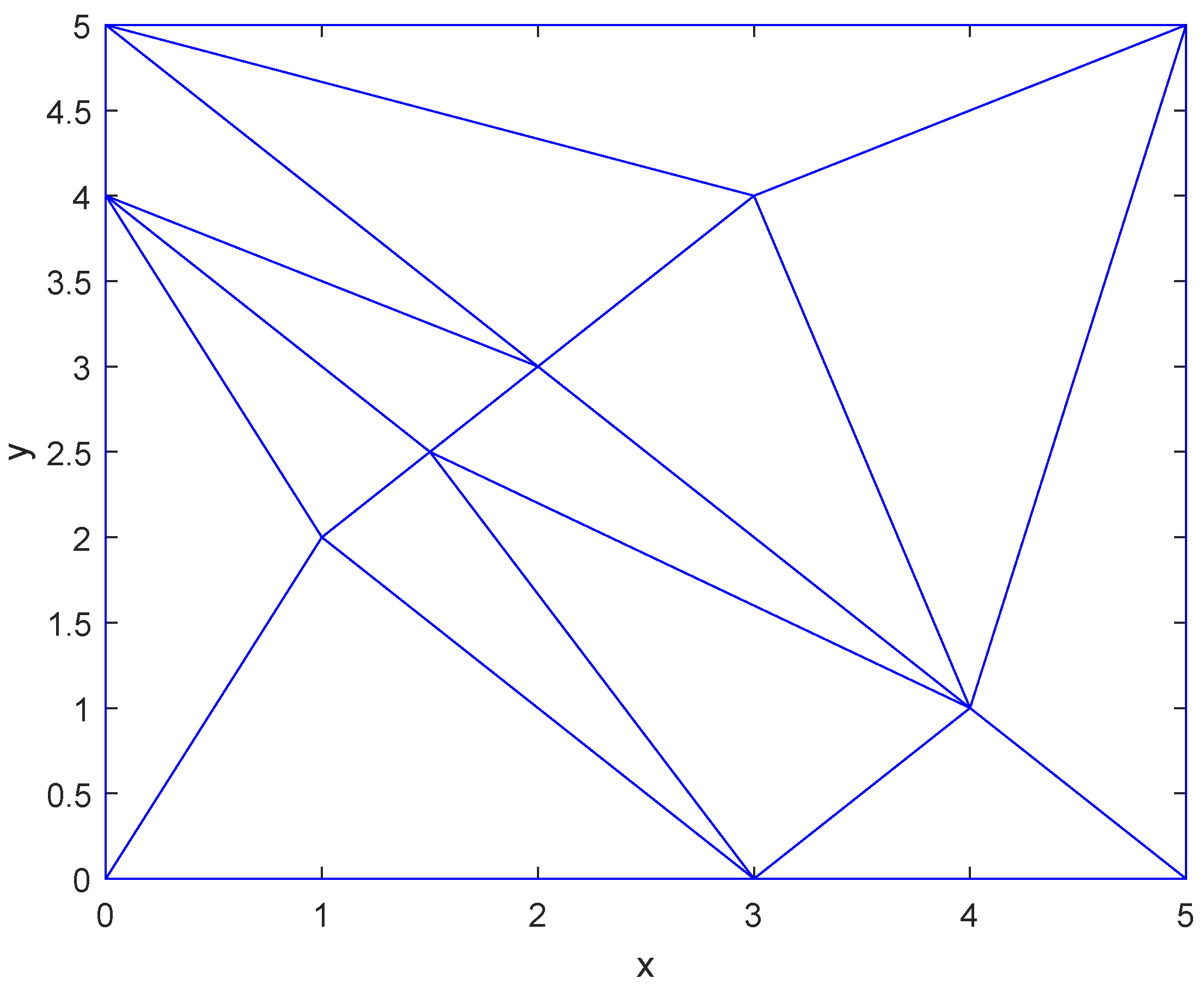
  $$T_0(0)=1,T_1(0)=0,T_2(0)=0,T_3(0)=0,$$

  $$T_0(1)=0,T_1(1)=1,T_2(1)=0,T_3(1)=0,$$

  $$T_0{}^{\prime }(0)=0,T_1{}^{\prime }(0)=0,T_2{}^{\prime }(0)=1,T_3{}^{\prime }(0)=0,$$

  $$T_0{}^{\prime }(1)=0,T_1{}^{\prime }(1)=0,T_2{}^{\prime }(1)=0,T_3{}^{\prime }(1)=1.$$

2.2. Two Classes of $C^1$ Coons Patches Constructions over Triangular Domain

There have been two classic methods for transfinite interpolation over triangular domain: side–side method proposed by BBG [8], also called parallel projection, and the side–vertex method proposed by Nielson [14], also called radial projection. For convenience, let $i,j,k=1,2,3,i\ne j\ne k\ne i$ in the rest of this paper.

2.2.1. Relationship between Barycentric Coordinates and Cartesian Coordinates

Let $\Delta T$ be a non-degenerate triangle with vertexes $V_i\left(x_i,y_i\right)\left(i=1,2,3\right)$. The vectors of three boundaries are marked as $e_1=V_3-V_2,e_2=V_1-V_3,e_3=V_2-V_1$. The side corresponding to the vertex $V_i$ is marked as $S_i$. The boundary of $\Delta T$ is marked as $\partial T$. The closure of $\Delta T$ is marked as $\overline{\mathrm{T}}$. For any point P inside $\Delta T$, mark the barycentric coordinates of P as $\left(b_1,b_2,b_3\right)$, where $b_i=\frac{A_i}{A}$, A is area of $\Delta T$, and $A_i$ is area of $\Delta P{V}_j{V}_k$. Mark cartesian coordinates of P as $(x,y)$. The relationships between the barycentric coordinates $\left(b_1,b_2,b_3\right)$ and the cartesian coordinates $(x,y)$ of P are as follows

$$\begin{array}{c}\hfill \left\{\begin{array}{c}x=b_1{x}_1+b_2{x}_2+b_3{x}_3,\hfill \\ y=b_1{y}_1+b_2{y}_2+b_3{y}_3,\hfill \\ 1=b_1+b_2+b_3,\hfill \end{array}\right.\end{array}$$

(4)

and

$$\begin{array}{c}\hfill {\mathrm{b}}_{\mathrm{i}}={\mathrm{b}}_{\mathrm{i}}\left(x,y\right)=\frac{\left|\begin{array}{cc}x-x_j& x-x_k\\ y-y_j& y-y_k\end{array}\right|}{\left|\begin{array}{cc}{x}_i-x_j& x_i-x_k\\ y_i-y_j& y_i-y_k\end{array}\right|}.\end{array}$$

(5)

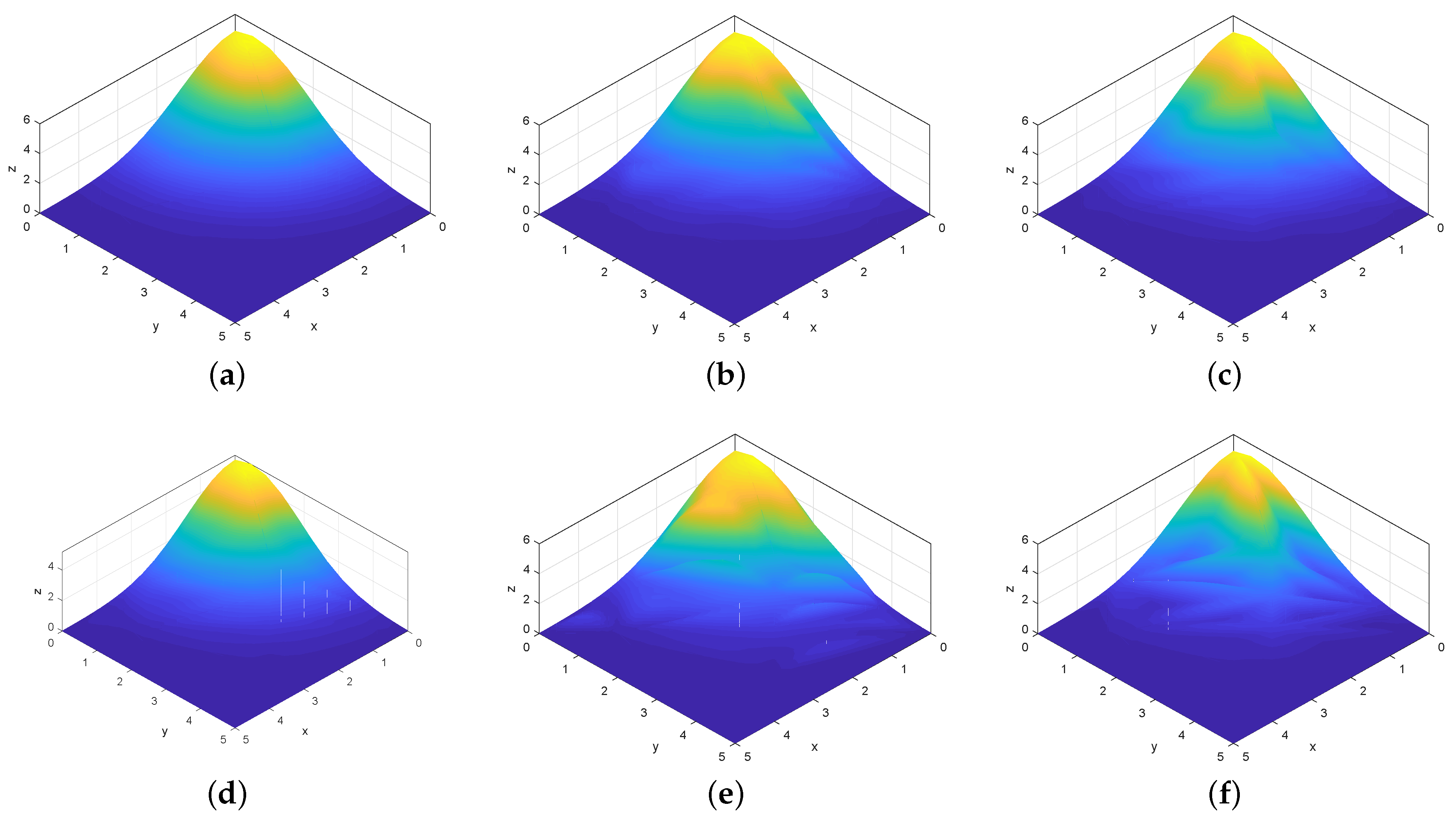
2.2.2. Coons Patch Construction Based on Side–Side Method

Given a function $F\left(x,y\right)$ over triangular domain $\Delta T$, side–side interpolant $P_i$ can be obtained by altering Hermite polynomial in BBG parallel projection method with the rational quadratic trigonometric Hermite functions in (1) as follows

$$\begin{array}{cc}\hfill P_1\left[F\right]& =T_0(\frac{b_3}{1-b_1})F\left(M_1\right)+T_1(\frac{b_3}{1-b_1})F\left(N_1\right)\hfill \\ \hfill & +T_2(\frac{b_3}{1-b_1})\left(1-b_1\right)\frac{\partial F}{\partial e_1}\left(M_1\right)+T_3(\frac{b_3}{1-b_1})\left(1-b_1\right)\frac{\partial F}{\partial e_1}\left(N_1\right),\hfill \end{array}$$

(6)

where $M_1=b_1{V}_1+\left(1-b_1\right)V_2,N_1=b_1{V}_1+\left(1-b_1\right)V_3,\frac{\partial F}{\partial e_1}\left(Q\right)$ is the partial derivative of F along the direction of $e_1$ at point Q. ${\alpha }_1$ and ${\beta }_1$ are shape parameters of $P_1\left[F\right]$.

$$\begin{array}{cc}\hfill P_2\left[F\right]& =T_0(\frac{b_1}{1-b_2})F\left(M_2\right)+T_1(\frac{b_1}{1-b_2})F\left(N_2\right)\hfill \\ \hfill & +T_2(\frac{b_1}{1-b_2})\left(1-b_2\right)\frac{\partial F}{\partial e_2}\left(M_2\right)+T_3(\frac{b_1}{1-b_2})\left(1-b_2\right)\frac{\partial F}{\partial e_2}\left(N_2\right),\hfill \end{array}$$

(7)

where $M_2=b_2{V}_2+\left(1-b_2\right)V_3,N_2=b_2{V}_2+\left(1-b_2\right)V_1,\frac{\partial F}{\partial e_2}\left(Q\right)$ is the partial derivative of F along the direction of $e_2$ at point Q. ${\alpha }_2$ and ${\beta }_2$ are shape parameters of $P_2\left[F\right]$.

$$\begin{array}{cc}\hfill P_3\left[F\right]& =T_0(\frac{b_2}{1-b_3})F\left(M_3\right)+T_1(\frac{b_2}{1-b_3})F\left(N_3\right)\hfill \\ \hfill & +T_2(\frac{b_2}{1-b_3})\left(1-b_3\right)\frac{\partial F}{\partial e_3}\left(M_3\right)+T_3(\frac{b_2}{1-b_3})\left(1-b_3\right)\frac{\partial F}{\partial e_3}\left(N_3\right),\hfill \end{array}$$

(8)

where $M_3=b_3{V}_3+\left(1-b_2\right)V_1,N_3=b_3{V}_3+\left(1-b_3\right)V_2,\frac{\partial F}{\partial e_3}\left(Q\right)$ is the partial derivative of F along the direction of $e_3$ at point Q. ${\alpha }_3$ and ${\beta }_3$ are shape parameters of $P_3\left[F\right]$.

The Coons patch is defined by the Boolean sum of $P_i\left[F\right](i=1,2,3)$ as follows

$$\begin{array}{c}\hfill P\left[F\right]={\omega }_1{P}_1\left[F\right]+{\omega }_2{P}_2\left[F\right]+{\omega }_3{P}_3\left[F\right],\end{array}$$

(9)

where ${\omega }_i\left(i=1,2,3\right)$ is called weight function and

$$\begin{array}{c}\hfill {\omega }_i={b_i}^2\left(3-2b_i+6b_j{b}_k\right),\end{array}$$

(10)

or

$$\begin{array}{c}\hfill {\omega }_i=\frac{{b_i}^2}{\sum _{n=1}^3{b_n}^2}.\end{array}$$

(11)

The weight function in (10) and (11) has the properties as follows

$$\begin{array}{c}\hfill \left\{\begin{array}{c}{\omega }_1+{\omega }_2+{\omega }_3=1,\\ {\omega }_i{|}_{e_i}=0,\\ \frac{\partial {\omega }_i}{\partial e_i}=0.\end{array}\right.\end{array}$$

(12)

Theorem 1.

Let $F\left(x,y\right)\in C^1(\partial T)$, when $\left(x,y\right)\in \partial T$, $P\left[F\right]$ in (9) interpolates to $F\left(x,y\right)$ and its first-order partial derivatives.

Proof of Theorem 1.

Consider any point on the side $S_i$, $i,j,k=1,2,3,i\ne j\ne k\ne i$, simple calculation gives that $b_1=0,b_2=1-b_3,$ and

$$\begin{array}{c}\hfill P\left[F\right]=\frac{{b_2}^2}{\sum _{n=1}^3{b_n}^2}{P}_2\left[F\right]+\frac{{b_3}^2}{\sum _{n=1}^3{b_n}^2}{P}_3\left[F\right].\end{array}$$

(13)

Direct computation gives that ${\left.P_j\left[F\right]\right|}_{e_i}=F\left(M_j\right),{\left.P_k\left[F\right]\right|}_{e_i}=F\left(N_k\right).$ It is easy to check that $M_j$ and $N_k$ are points on the side $S_i$, thus

$$\begin{array}{c}\hfill P\left[F\right]=\frac{{b_2}^2}{\sum _{n=1}^3{b_n}^2}F\left(M_j\right)+\frac{{b_3}^2}{\sum _{n=1}^3{b_n}^2}F\left(N_k\right)=F\left(S_i\right).\end{array}$$

(14)

Therefore,

$$\begin{array}{c}\hfill {\left.P\left[F\right]\right|}_{\partial T}={\left.F\right|}_{\partial T}.\end{array}$$

(15)

According to (12), we have

$$\begin{array}{cc}\hfill {\left.\partial P\left[F\right]\right|}_{e_i}& =\partial {\left.\left({\omega }_i{P}_i\left[F\right]\right)\right|}_{e_i}+\partial {\left.\left({\omega }_j{P}_j\left[F\right]\right)\right|}_{e_i}+\partial {\left.\left({\omega }_k{P}_k\left[F\right]\right)\right|}_{e_i}\hfill \\ \hfill & ={\left.\partial {\omega }_j{P}_j\left[F\right]\right|}_{e_i}+{\left.{\omega }_j\partial P_j\left[F\right]\right|}_{e_i}+{\left.\partial {\omega }_k{P}_k\left[F\right]\right|}_{e_i}+{\left.{\omega }_k\partial P_k\left[F\right]\right|}_{e_i}\hfill \\ \hfill & =\partial F\left(S_i\right).\hfill \end{array}$$

(16)

Therefore, we have

$$\begin{array}{c}\hfill {\left.\partial P\left[F\right]\right|}_{\partial T}={\left.\partial F\right|}_{\partial T}.\end{array}$$

(17)

These imply the theorem. □

Detailed proof can be referenced from [11]. We call the interpolation method of (9) as the side–side method for interpolation based on the rational quadratic trigonometric Hermite functions (SS).

2.2.3. Coons Patch Construction Based on Side–Vertex Method

Consider the point on the side $S_i$ corresponding to the vertex $V_i$, and the coordinates of $S_i$ are follows

$$\begin{array}{c}\hfill S_i=S_i(x,y)=(\frac{x-b_i{x}_i}{1-b_i},\frac{y-b_i{y}_i}{1-b_i})=(\frac{b_j{x}_j-b_k{x}_k}{b_j+b_k},\frac{b_j{y}_j-b_k{y}_k}{b_j+b_k}).\end{array}$$

(18)

Now, alter the cubic Hermite polynomial of the interpolants in radial projection method by the following interpolants,

$$\begin{array}{c}\hfill D_i\left[F\right]=T_1(1-b_i)F(S_i)+T_3(1-b_i)R_i{}^{\prime }(1)+T_1(b_i)F(V_i)-T_3(b_i)R_i{}^{\prime }(0),\end{array}$$

(19)

where $(i=1,2,3)$, ${\alpha }_i$ and ${\beta }_i$$(i=1,2,3)$ are shape parameters of $D_i\left[F\right]$, and

$$\begin{array}{c}\hfill \left\{\begin{array}{c}{R_i}^{\prime }(1)=\frac{(x-x_i)F_x(S_i)+(y-y_i)F_y(S_i)}{1-b_i},\hfill \\ {R_i}^{\prime }(0)=\frac{(x-x_i)F_x(V_i)+(y-y_i)F_y(V_i)}{1-b_i}..\hfill \end{array}\right.\end{array}$$

(20)

The Coons patch is defined by the Boolean sum of $D_i\left[F\right](i=1,2,3)$ as follows

$$\begin{array}{c}\hfill D\left[F\right]={\overline{\omega }}_1{D}_1\left[F\right]+{\overline{\omega }}_2{D}_2\left[F\right]+{\overline{\omega }}_3{D}_3\left[F\right],\end{array}$$

(21)

where ${\omega }_i\left(i=1,2,3\right)$ is called weight function and

$$\begin{array}{c}\hfill {\overline{\omega }}_i=\frac{1/{b_i}^2}{1/{b_1}^2+1/{b_2}^2+1/{b_3}^2},\end{array}$$

(22)

or

$$\begin{array}{c}\hfill {\overline{\omega }}_i=\frac{{b_j}^2{b_k}^2}{{b_2}^2{b_3}^2+{b_1}^2{b_3}^2+{b_2}^2{b_1}^2}.\end{array}$$

(23)

The above weight function has the properties as follows

$$\begin{array}{c}\hfill \left\{\begin{array}{c}{\overline{\omega }}_1+{\overline{\omega }}_2+{\overline{\omega }}_3=1,\\ {\overline{\omega }}_i{{|}_e}_{{}_i}={\delta }_{ij},\\ \frac{\partial {\overline{\omega }}_i}{\partial e_i}=0.\end{array}\right.\end{array}$$

(24)

Theorem 2.

Let $F\left(x,y\right)\in C^1(\partial T)$, when $\left(x,y\right)\in \partial T$, $D\left[F\right]$ in (21) interpolates $F\left(x,y\right)$ and its first-order partial derivatives.

Proof of Theorem 2.

The proof of Theorem 2 is analogy to Theorem 1. Detailed proof can be referenced from [14]. □

We call the interpolation method of (21) as side–vertex method for interpolation based on the rational quadratic trigonometric Hermite functions (SV).

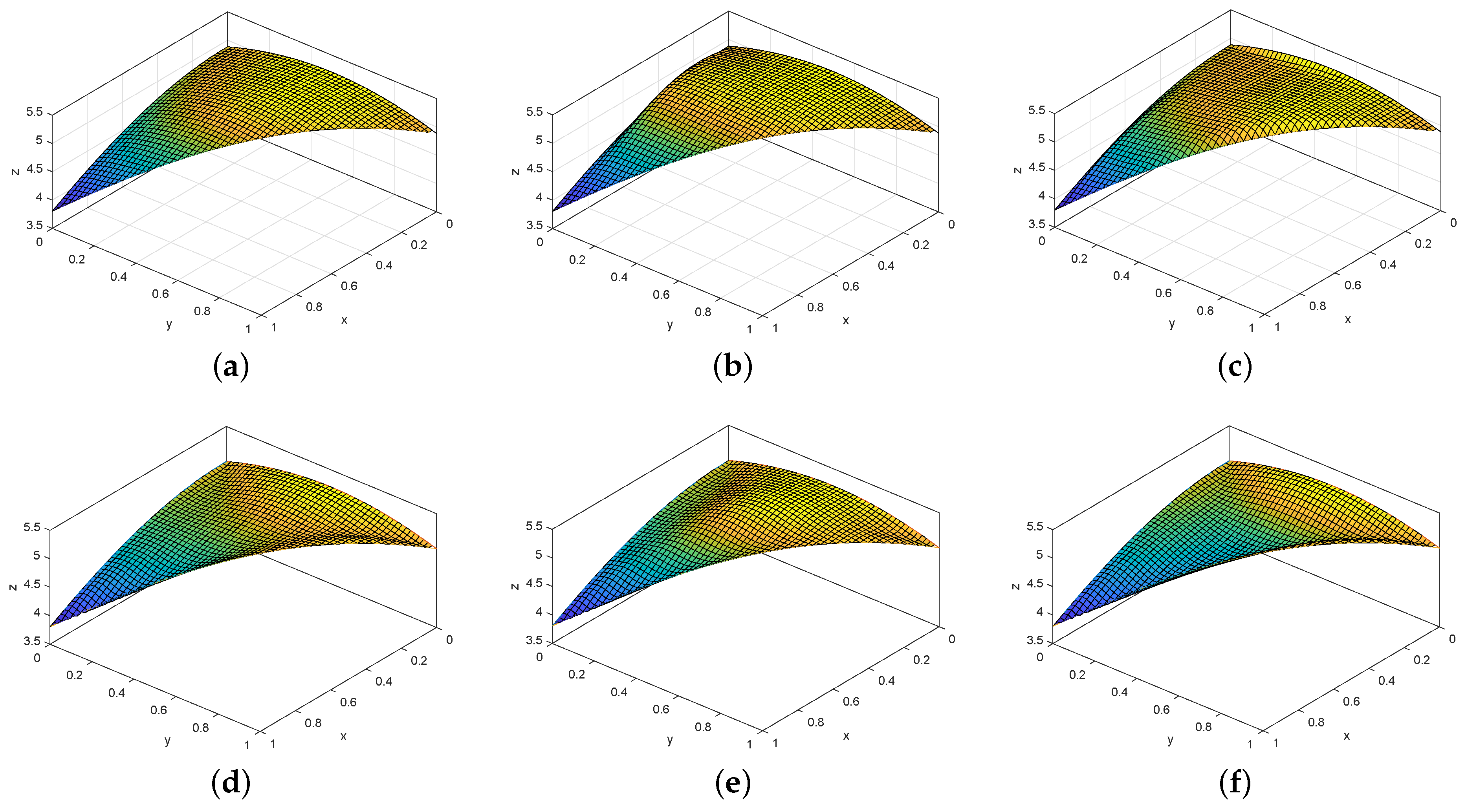
2.3. Region Control of Shape Parameters

In order to deal with the problem of well-posedness in image zooming, we give the region control of the shape parameters using the method proposed in [27]. For the gray-scale values of the new pixels should be bounded between 0 and 255 for eight-bit images, we constrain the interpolants $P_i\left[F\right]$ and $D_i\left[F\right]$ to lie between the two given piecewise step functions. For any $x\in \left[x_r,x_{r+1}\right],t=\left(x-x_r\right)/h_r,r=1,2,\dots ,n-1$, we alter the piecewise interpolation curves given in [27] with $g\left(x\right)=g_r$ and $g^{\ast }\left(x\right)=g_r^{\ast }$, where $g_r<F<g_r^{\ast }$, $S=S\left(t\right)=sin\left(\frac{\pi }{2}t\right)$ and $C=C\left(t\right)=cos\left(\frac{\pi }{2}t\right)$. For SS, if the interpolant $P_i\left[F\right],i=1,2,3,$ satisfies

$$\begin{array}{c}\hfill g\left(x\right)<P_i\left[F\right]<g^{\ast }\left(x\right),\end{array}$$

(25)

for any $x\in \left[x_1,x_n\right]$, then $P_i\left[F\right]$ is called the constrained interpolant lying strictly between the two given piecewise step functions $g\left(x\right)$ and $g^{\ast }\left(x\right)$.

For $x\in \left[x_r,x_{r+1}\right],1\le r\le n-1$, $P_i\left[F\right]$ lies strictly above the piecewise step function $g\left(x\right)=g_r$, if $P_i\left[F\right]>g_r$, which is equivalent to

$$\begin{array}{cc}\hfill P_i\left[F\right]-g_r& =T_0(t)F\left(M_i\right)+T_1(t)F\left(N_i\right)+T_2(t)\left(1-b_i\right)\frac{\partial F}{\partial e_i}\left(M_i\right)+T_3(t)\left(1-b_i\right)\frac{\partial F}{\partial e_i}\left(N_i\right)-g_r\hfill \\ \hfill & =\left[\begin{array}{c}{\alpha }_{i}F\left(M_i\right)C^2+{\beta }_{i}F\left(N_i\right)S^2\hfill \\ +\frac{\pi }{2}{\alpha }_i\left(1-b_i\right)\frac{\partial F\left(M_i\right)}{\partial e_i}S\left(1-S\right)\hfill \\ \begin{array}{c}-\frac{\pi }{2}{\beta }_i\left(1-b_i\right)\frac{\partial F\left(N_i\right)}{\partial e_i}C\left(1-C\right)\hfill \\ -\left({\alpha }_i{C}^2+{\beta }_i{S}^2\right)g_r\hfill \end{array}\hfill \end{array}\right]\frac{1}{{\alpha }_i{C}^2+{\beta }_i{S}^2}\hfill \\ \hfill & \ge \left[\begin{array}{c}\begin{array}{c}{\alpha }_{i}F\left(M_i\right)C^2+{\beta }_{i}F\left(N_i\right)S^2\hfill \\ -\frac{\pi }{2}{\alpha }_i\left|\frac{\partial F\left(M_i\right)}{\partial e_i}\right|S\left(1-S\right)\hfill \\ -\frac{\pi }{2}{\beta }_i\left|\frac{\partial F\left(N_i\right)}{\partial e_i}\right|C\left(1-C\right)\hfill \end{array}\hfill \\ -\left({\alpha }_i{C}^2+{\beta }_i{S}^2\right)g_r\hfill \end{array}\right]\frac{1}{{\alpha }_i{C}^2+{\beta }_i{S}^2}\hfill \\ \hfill & =\left\{\begin{array}{c}\begin{array}{c}{\alpha }_{i}F\left(M_i\right)C^2+{\beta }_{i}F\left(N_i\right)S^2\hfill \\ +\frac{1}{\pi }{\alpha }_i\left|\frac{\partial F\left(M_i\right)}{\partial e_i}\right|{\left(S-1\right)}^2-\frac{1}{\pi }{\alpha }_i\left|\frac{\partial F\left(M_i\right)}{\partial e_i}\right|S^2-\frac{1}{\pi }{\alpha }_i\left|\frac{\partial F\left(M_i\right)}{\partial e_i}\right|\left(S^2+C^2\right)\hfill \\ +\frac{1}{\pi }{\beta }_i\left|\frac{\partial F\left(N_i\right)}{\partial e_i}\right|{\left(C-1\right)}^2-\frac{1}{\pi }{\beta }_i\left|\frac{\partial F\left(N_i\right)}{\partial e_i}\right|C^2-\frac{1}{\pi }{\beta }_i\left|\frac{\partial F\left(N_i\right)}{\partial e_i}\right|\left(S^2+C^2\right)\hfill \end{array}\hfill \\ -{\alpha }_i{C}^2{g}_r-{\beta }_i{S}^2{g}_r\hfill \end{array}\right\}\frac{1}{{\alpha }_i{C}^2+{\beta }_i{S}^2}\hfill \\ \hfill & =\left\{\begin{array}{c}\frac{1}{\pi }{\alpha }_i\left|\frac{\partial F\left(M_i\right)}{\partial e_i}\right|{\left(S-1\right)}^2+\frac{1}{\pi }{\beta }_i\left|\frac{\partial F\left(N_i\right)}{\partial e_i}\right|{\left(C-1\right)}^2\hfill \\ +C^2\left[{\alpha }_{i}F\left(M_i\right)-\frac{1}{\pi }{\alpha }_i\left|\frac{\partial F\left(M_i\right)}{\partial e_i}\right|-\frac{2}{\pi }{\beta }_i\left|\frac{\partial F\left(N_i\right)}{\partial e_i}\right|-{\alpha }_i{g}_r\right]\hfill \\ +S^2\left[{\beta }_{i}F\left(N_i\right)-\frac{2}{\pi }{\alpha }_i\left|\frac{\partial F\left(M_i\right)}{\partial e_i}\right|-\frac{1}{\pi }{\beta }_i\left|\frac{\partial F\left(N_i\right)}{\partial e_i}\right|-{\beta }_i{g}_r\right]\hfill \end{array}\right\}\frac{1}{{\alpha }_i{C}^2+{\beta }_i{S}^2}.\hfill \\ \hfill \end{array}$$

We can obtain the following sufficient conditions for $P_i\left[F\right]>g_r,\forall x\in \left[x_r,x_{r+1}\right]$

$$\begin{array}{c}\hfill \left\{\begin{array}{c}0<{\alpha }_i<\frac{\pi }{2}\frac{F\left(N_i\right)-\frac{1}{\pi }\left|\frac{\partial F\left(N_i\right)}{\partial e_i}\right|-g_r}{\left|\frac{\partial F\left(M_i\right)}{\partial e_i}\right|}{\beta }_i,\\ 0<{\beta }_i<\frac{\pi }{2}\frac{F\left(M_i\right)-\frac{1}{\pi }\left|\frac{\partial F\left(M_i\right)}{\partial e_i}\right|-g_r}{\left|\frac{\partial F\left(N_i\right)}{\partial e_i}\right|}{\alpha }_i.\end{array}\right.\end{array}$$

(26)

Similarly, for $x\in \left[x_r,x_{r+1}\right],1\le r\le n-1$, the interpolant $P_i\left[F\right]$ lies strictly below the piecewise step function $g^{\ast }\left(x\right)=g_r^{\ast }$, if $P_i\left[F\right]<g_r^{\ast }$, which is equivalent to

$$\begin{array}{cc}\hfill g_r^{\ast }-P_i\left[F\right]& =g_r^{\ast }-T_0(t)F\left(M_i\right)-T_1(t)F\left(N_i\right)-T_2(t)\left(1-b_i\right)\frac{\partial F}{\partial e_i}\left(M_i\right)-T_3(t)\left(1-b_i\right)\frac{\partial F}{\partial e_i}\left(N_i\right)\hfill \\ \hfill & \ge \left[\begin{array}{c}\begin{array}{c}\left({\alpha }_i{C}^2+{\beta }_i{S}^2\right)g_r^{\ast }\hfill \\ -{\alpha }_{i}F\left(M_i\right)C^2-{\beta }_{i}F\left(N_i\right)S^2\hfill \end{array}\hfill \\ -\frac{\pi }{2}{\alpha }_i\left|\frac{\partial F\left(M_i\right)}{\partial e_i}\right|S\left(1-S\right)\hfill \\ -\frac{\pi }{2}{\beta }_i\left|\frac{\partial F\left(N_i\right)}{\partial e_i}\right|C\left(1-C\right)\hfill \end{array}\right]\frac{1}{{\alpha }_i{C}^2+{\beta }_i{S}^2}\hfill \\ \hfill & =\left\{\begin{array}{c}\frac{1}{\pi }{\alpha }_i\left|\frac{\partial F\left(M_i\right)}{\partial e_i}\right|{\left(S-1\right)}^2+\frac{1}{\pi }{\beta }_i\left|\frac{\partial F\left(N_i\right)}{\partial e_i}\right|{\left(C-1\right)}^2\hfill \\ +C^2\left[-{\alpha }_{i}F\left(M_i\right)-\frac{1}{\pi }{\alpha }_i\left|\frac{\partial F\left(M_i\right)}{\partial e_i}\right|-\frac{2}{\pi }{\beta }_i\left|\frac{\partial F\left(N_i\right)}{\partial e_i}\right|+{\alpha }_i{g}_r^{\ast }\right]\hfill \\ +S^2\left[-{\beta }_{i}F\left(N_i\right)-\frac{2}{\pi }{\alpha }_i\left|\frac{\partial F\left(M_i\right)}{\partial e_i}\right|-\frac{1}{\pi }{\beta }_i\left|\frac{\partial F\left(N_i\right)}{\partial e_i}\right|+{\beta }_i{g}_r^{\ast }\right]\hfill \end{array}\right\}\frac{1}{{\alpha }_i{C}^2+{\beta }_i{S}^2}.\hfill \end{array}$$

We can obtain the following sufficient conditions for $g_r^{\ast }-P_i\left[F\right]>0,\forall x\in \left[x_r,x_{r+1}\right]$

$$\begin{array}{c}\hfill \left\{\begin{array}{c}0<{\alpha }_i<\frac{\pi }{2}\frac{g_r^{\ast }-F\left(N_i\right)-\frac{1}{\pi }\left|\frac{\partial F\left(N_i\right)}{\partial e_i}\right|}{\left|\frac{\partial F\left(M_i\right)}{\partial e_i}\right|}{\beta }_i,\\ 0<{\beta }_i<\frac{\pi }{2}\frac{g_r^{\ast }-F\left(M_i\right)-\frac{1}{\pi }\left|\frac{\partial F\left(M_i\right)}{\partial e_i}\right|}{\left|\frac{\partial F\left(N_i\right)}{\partial e_i}\right|}{\alpha }_i.\end{array}\right.\end{array}$$

(27)

Therefore, (26)–(27) are the sufficient conditions to ensure $g\left(x\right)<P_i\left[F\right]<g^{\ast }\left(x\right)$.

For SV, if the interpolant $D_i\left[F\right],i=1,2,3,$ satisfies

$$\begin{array}{c}\hfill g\left(x\right)<D_i\left[F\right]<g^{\ast }\left(x\right),\end{array}$$

(28)

for any $x\in \left[x_1,x_n\right]$, then $D_i\left[F\right]$ is called the constrained interpolant lying strictly between the two given piecewise step functions $g\left(x\right)$ and $g^{\ast }\left(x\right)$.

For $x\in \left[x_r,x_{r+1}\right],1\le r\le n-1$, $D_i\left[F\right]$ lies strictly above the piecewise step function $g(x)=g_r$, if $D_i\left[F\right]>g_r$, which is equivalent to

$$\begin{array}{cc}\hfill D_i\left[F\right]-g_r& =T_1(1-t)F\left(S_i\right)+T_3(1-t){R_i}^{\prime }\left(1\right)+T_1(t)F\left(V_i\right)-T_3(t){R_i}^{\prime }\left(0\right)-g_r\hfill \\ \hfill & =\frac{{\beta }_i{C}^2}{{\alpha }_i{S}^2+{\beta }_i{C}^2}F\left(S_i\right)-\frac{2}{\pi }\frac{{\beta }_{i}S\left(1-S\right)}{{\alpha }_i{S}^2+{\beta }_i{C}^2}{R_i}^{\prime }\left(1\right)+\frac{{\beta }_i{S}^2}{{\alpha }_i{C}^2+{\beta }_i{S}^2}F\left(V_i\right)\hfill \\ \hfill & +\frac{2}{\pi }\frac{{\beta }_{i}C\left(1-C\right)}{{\alpha }_i{C}^2+{\beta }_i{S}^2}{R_i}^{\prime }\left(0\right)-g_r\left(S^2+C^2\right)\hfill \\ \hfill & =\left[\begin{array}{c}{\beta }_{i}F\left(S_i\right)C^2\hfill \\ -\frac{2}{\pi }{\beta }_i{R_i}^{\prime }\left(1\right)S\left(1-S\right)\hfill \\ -C^2{g}_r\left({\alpha }_i{S}^2+{\beta }_i{C}^2\right)\hfill \end{array}\right]\frac{1}{{\alpha }_i{S}^2+{\beta }_i{C}^2}\hfill \\ \hfill & +\left[\begin{array}{c}{\beta }_{i}F\left(V_i\right)S^2\hfill \\ +\frac{2}{\pi }{\beta }_i{R_i}^{\prime }\left(0\right)C\left(1-C\right)\hfill \\ -S^2{g}_r\left({\alpha }_i{C}^2+{\beta }_i{S}^2\right)\hfill \end{array}\right]\frac{1}{{\alpha }_i{C}^2+{\beta }_i{S}^2}\hfill \\ \hfill & \ge \left[\begin{array}{c}{\beta }_{i}F\left(S_i\right)C^2\hfill \\ -\frac{2}{\pi }{\beta }_i\left|{R_i}^{\prime }\left(1\right)\right|S\left(1-S\right)\hfill \\ -C^2{g}_r\left({\alpha }_i{S}^2+{\beta }_i{C}^2\right)\hfill \end{array}\right]\frac{1}{{\alpha }_i{S}^2+{\beta }_i{C}^2}\hfill \\ \hfill & +\left[\begin{array}{c}{\beta }_{i}F\left(V_i\right)S^2\hfill \\ -\frac{2}{\pi }{\beta }_i\left|{R_i}^{\prime }\left(0\right)\right|C\left(1-C\right)\hfill \\ -S^2{g}_r\left({\alpha }_i{C}^2+{\beta }_i{S}^2\right)\hfill \end{array}\right]\frac{1}{{\alpha }_i{C}^2+{\beta }_i{S}^2}\hfill \\ \hfill & =\left\{\begin{array}{c}\frac{1}{\pi }{\beta }_i\left|{R_i}^{\prime }\left(1\right)\right|{\left(S-1\right)}^2\hfill \\ +C^2\left[-\frac{1}{\pi }{\beta }_i\left|{R_i}^{\prime }\left(1\right)\right|+{\beta }_{i}F\left(S_i\right)-{\alpha }_i{g}_r+\left({\alpha }_i-{\beta }_i\right)g_r{C}^2\right]\hfill \end{array}\right\}\frac{1}{{\alpha }_i{S}^2+{\beta }_i{C}^2}\hfill \\ \hfill & +\left\{\begin{array}{c}\frac{1}{\pi }{\beta }_i\left|{R_i}^{\prime }\left(0\right)\right|{\left(C-1\right)}^2\hfill \\ +S^2\left[-\frac{1}{\pi }{\beta }_i\left|{R_i}^{\prime }\left(0\right)\right|+{\beta }_{i}F\left(V_i\right)-{\alpha }_i{g}_r+\left({\alpha }_i-{\beta }_i\right)g_r{S}^2\right]\hfill \end{array}\right\}\frac{1}{{\alpha }_i{C}^2+{\beta }_i{S}^2}\hfill \\ \hfill & \ge \left\{\begin{array}{c}\frac{1}{\pi }{\beta }_i\left|{R_i}^{\prime }\left(1\right)\right|{\left(S-1\right)}^2\hfill \\ +C^2\left[-\frac{1}{\pi }{\beta }_i\left|{R_i}^{\prime }\left(1\right)\right|+{\beta }_{i}F\left(S_i\right)-g_r\left(2{\alpha }_i-{\beta }_i\right)\right]\hfill \end{array}\right\}\frac{1}{{\alpha }_i{S}^2+{\beta }_i{C}^2}\hfill \\ \hfill & +\left\{\begin{array}{c}\frac{1}{\pi }{\beta }_i\left|{R_i}^{\prime }\left(0\right)\right|{\left(C-1\right)}^2\hfill \\ +S^2\left[-\frac{1}{\pi }{\beta }_i\left|{R_i}^{\prime }\left(0\right)\right|+{\beta }_{i}F\left(V_i\right)-g_r\left(2{\alpha }_i-{\beta }_i\right)\right]\hfill \end{array}\right\}\frac{1}{{\alpha }_i{C}^2+{\beta }_i{S}^2}.\hfill \end{array}$$

We can obtain the following sufficient conditions for $D_i\left[F\right]-g_r>0,\forall x\in \left[x_r,x_{r+1}\right]$

$$\begin{array}{c}\hfill \left\{\begin{array}{c}{\beta }_i>0,\\ 0<{\alpha }_i<min\left\{\frac{g_r+F\left(S_i\right)-\frac{1}{\pi }\left|{R_i}^{\prime }\left(1\right)\right|}{2g_r}{\beta }_i,\frac{g_r+F\left(V_i\right)-\frac{1}{\pi }\left|{R_i}^{\prime }\left(0\right)\right|}{2g_r}{\beta }_i\right\}.\end{array}\right.\end{array}$$

(29)

Similarly, $D_i\left[F\right]$ lies strictly below the piecewise step function $g^{\ast }\left(x\right)=g_r^{\ast }$, if $g_r^{\ast }-D_i\left[F\right]>0,$ which is equivalent to

$$\begin{array}{cc}\hfill g_r^{\ast }-D_i\left[F\right]& =g_r^{\ast }-T_1(1-t)F\left(S_i\right)-T_3(1-t){R_i}^{\prime }\left(1\right)-T_1(t)F\left(V_i\right)+T_3(t){R_i}^{\prime }\left(0\right)\hfill \\ \hfill & =g_r^{\ast }\left(S^2+C^2\right)-\frac{{\beta }_i{C}^2}{{\alpha }_i{S}^2+{\beta }_i{C}^2}F\left(S_i\right)+\frac{2}{\pi }\frac{{\beta }_{i}S\left(1-S\right)}{{\alpha }_i{S}^2+{\beta }_i{C}^2}{R_i}^{\prime }\left(1\right)\hfill \\ \hfill & -\frac{{\beta }_i{S}^2}{{\alpha }_i{C}^2+{\beta }_i{S}^2}F\left(V_i\right)-\frac{2}{\pi }\frac{{\beta }_{i}C\left(1-C\right)}{{\alpha }_i{C}^2+{\beta }_i{S}^2}{R_i}^{\prime }\left(0\right)\hfill \\ \hfill & =\left[\begin{array}{c}-{\beta }_{i}F\left(S_i\right)C^2\hfill \\ +\frac{2}{\pi }{\beta }_i{R_i}^{\prime }\left(1\right)S\left(1-S\right)\hfill \\ +C^2{g}_r^{\ast }\left({\alpha }_i{S}^2+{\beta }_i{C}^2\right)\hfill \end{array}\right]\frac{1}{{\alpha }_i{S}^2+{\beta }_i{C}^2}\hfill \\ \hfill & +\left[\begin{array}{c}-{\beta }_{i}F\left(V_i\right)S^2\hfill \\ -\frac{2}{\pi }{\beta }_i{R_i}^{\prime }\left(0\right)C\left(1-C\right)\hfill \\ +S^2{g}_r^{\ast }\left({\alpha }_i{C}^2+{\beta }_i{S}^2\right)\hfill \end{array}\right]\frac{1}{{\alpha }_i{C}^2+{\beta }_i{S}^2}\hfill \\ \hfill & \ge \left[\begin{array}{c}-{\beta }_{i}F\left(S_i\right)C^2\hfill \\ -\frac{2}{\pi }{\beta }_i\left|{R_i}^{\prime }\left(1\right)\right|S\left(1-S\right)\hfill \\ +C^2{g}_r^{\ast }\left({\alpha }_i{S}^2+{\beta }_i{C}^2\right)\hfill \end{array}\right]\frac{1}{{\alpha }_i{S}^2+{\beta }_i{C}^2}\hfill \\ \hfill & +\left[\begin{array}{c}-{\beta }_{i}F\left(V_i\right)S^2\hfill \\ -\frac{2}{\pi }{\beta }_i\left|{R_i}^{\prime }\left(0\right)\right|C\left(1-C\right)\hfill \\ +S^2{g}_r^{\ast }\left({\alpha }_i{C}^2+{\beta }_i{S}^2\right)\hfill \end{array}\right]\frac{1}{{\alpha }_i{C}^2+{\beta }_i{S}^2}\hfill \\ \hfill & =\left\{\begin{array}{c}\frac{1}{\pi }{\beta }_i\left|{R_i}^{\prime }\left(1\right)\right|{\left(S-1\right)}^2+g_r^{\ast }\left[\left({\alpha }_i-{\beta }_i\right)C^2+{\alpha }_i\right]\hfill \\ +C^2\left[-\frac{1}{\pi }{\beta }_i\left|{R_i}^{\prime }\left(1\right)\right|+{\beta }_{i}F\left(S_i\right)+g_r^{\ast }\left[-2{\alpha }_i+{\beta }_i-\left({\alpha }_i-{\beta }_i\right)S^2\right]\right]\hfill \end{array}\right\}\frac{1}{{\alpha }_i{S}^2+{\beta }_i{C}^2}\hfill \\ \hfill & +\left\{\begin{array}{c}\frac{1}{\pi }{\beta }_i\left|{R_i}^{\prime }\left(0\right)\right|{\left(C-1\right)}^2+g_r^{\ast }\left[\left({\alpha }_i-{\beta }_i\right)S^2+{\alpha }_i\right]\hfill \\ +S^2\left[-\frac{1}{\pi }{\beta }_i\left|{R_i}^{\prime }\left(0\right)\right|+{\beta }_{i}F\left(V_i\right)+g_r^{\ast }\left[-2{\alpha }_i+{\beta }_i-\left({\alpha }_i-{\beta }_i\right)C^2\right]\right]\hfill \end{array}\right\}\frac{1}{{\alpha }_i{C}^2+{\beta }_i{S}^2}\hfill \\ \hfill & \ge \left\{\begin{array}{c}\frac{1}{\pi }{\beta }_i\left|{R_i}^{\prime }\left(1\right)\right|{\left(S-1\right)}^2+{\beta }_i{g}_r^{\ast }\hfill \\ +C^2\left[-\frac{1}{\pi }{\beta }_i\left|{R_i}^{\prime }\left(1\right)\right|+{\beta }_{i}F\left(S_i\right)+g_r^{\ast }\left[-3{\alpha }_i+2{\beta }_i\right]\right]\hfill \end{array}\right\}\frac{1}{{\alpha }_i{S}^2+{\beta }_i{C}^2}\hfill \\ \hfill & +\left\{\begin{array}{c}\frac{1}{\pi }{\beta }_i\left|{R_i}^{\prime }\left(0\right)\right|{\left(C-1\right)}^2+{\beta }_i{g}_r^{\ast }\hfill \\ +S^2\left[-\frac{1}{\pi }{\beta }_i\left|{R_i}^{\prime }\left(0\right)\right|+{\beta }_{i}F\left(V_i\right)+g_r^{\ast }\left[-3{\alpha }_i+2{\beta }_i\right]\right]\hfill \end{array}\right\}\frac{1}{{\alpha }_i{C}^2+{\beta }_i{S}^2}.\hfill \end{array}$$

We can obtain the following sufficient conditions for $g_r^{\ast }-D_i\left[F\right]>0,\forall x\in \left[x_r,x_{r+1}\right]$

$$\begin{array}{c}\hfill \left\{\begin{array}{c}{\beta }_i>0,\\ 0<{\alpha }_i<min\left\{\frac{2g_r^{\ast }+F\left(S_i\right)-\frac{1}{\pi }\left|{R_i}^{\prime }\left(1\right)\right|}{3g_r^{\ast }}{\beta }_i,\frac{2g_r^{\ast }+F\left(V_i\right)-\frac{1}{\pi }\left|{R_i}^{\prime }\left(0\right)\right|}{3g_r^{\ast }}{\beta }_i\right\}.\end{array}\right.\end{array}$$

(30)

Therefore, (29)–(30) are the sufficient conditions to ensure $g\left(x\right)<D_i\left[F\right]<g^{\ast }\left(x\right)$.

2.4. Image Zooming Based on Two Classes of Coons Patches Construction over Triangular Domain

Coons patches constructed by the proposed method can be also applied in image interpolation and image zooming. This work mainly discusses the problem of gray-scale images zooming.

Image zooming results using different methods will be compared by the visual quality, edge detection by Prewitt operator and calculating peak signal to noise ratio (PSNR), structural similarity index (SSIM), feature similarity (FSIM) [28], multiscale structural similarity (MS-SSIM) [29].

PSNR is a full reference image quality evaluation index, which is defined as follows

$$\begin{array}{c}\hfill \mathrm{MSE}=\frac{1}{H\times W}\sum _{i=1}^H\sum _{j=1}^W{(X(i,j)-Y(i,j))}^2,\end{array}$$

(31)

$$\begin{array}{c}\hfill PSNR=10{log}_{10}(\frac{{(2^n-1)}^2}{MSE}),\end{array}$$

(32)

where MSE is the square error between the magnified HR image and the original image. H and W is the height and the width of the image; X is the magnified HR image; Y is the original image; n is the bit num of pixel.

SSIM measures the image similarity from brightness l, contrast c and structure s, which are defined as follows

$$\begin{array}{c}\hfill l(X,Y)=\frac{2{\mu }_X{\mu }_Y+C_1}{{\mu }_X^2+{\mu }_Y^2+C_1},\end{array}$$

(33)

$$\begin{array}{c}\hfill c(X,Y)=\frac{2{\mu }_X{\mu }_Y+C_2}{{\mu }_X^2+{\mu }_Y^2+C_2},\end{array}$$

(34)

$$\begin{array}{c}\hfill s(X,Y)=\frac{{\sigma }_{XY}+C_3}{{\sigma }_X{\sigma }_Y+C_3},\end{array}$$

(35)

where $\mu x$ and $\mu y$ are mean of X and Y respectively; $\sigma X$ and $\sigma Y$ are variance of X and Y respectively; $\sigma XY$ is covariance of X and Y; $C_1={\left(k_1\ast L\right)}^2$, $C_2={\left(k_2\ast L\right)}^2$ and $C_3=C_2/2$, where $k_1=0.01$, $k_2=0.03$ and $L=225$. Therefore SSIM is defined as follows

$$\begin{array}{c}\hfill SSIM=l\left(X,Y\right)\ast c\left(X,Y\right)\ast s\left(X,Y\right).\end{array}$$

(36)

Higher PSNR and SSIM means a better quality image.

To further demonstrate the proposed method can preserve image edge details, we use a Prewitt operator to detect the edges of the image zooming results. The Prewitt operator is used in image processing, particularly within edge detection algorithms. Technically, it is a discrete differentiation operator, computing an approximation of the gradient of the image intensity function. At each point in the image, the result of the Prewitt operator is either the corresponding gradient vector or the norm of this vector. More edge details that Prewitt operator can detect means more edge details preserved.

Method of Image Zooming by Coons Patch Construction

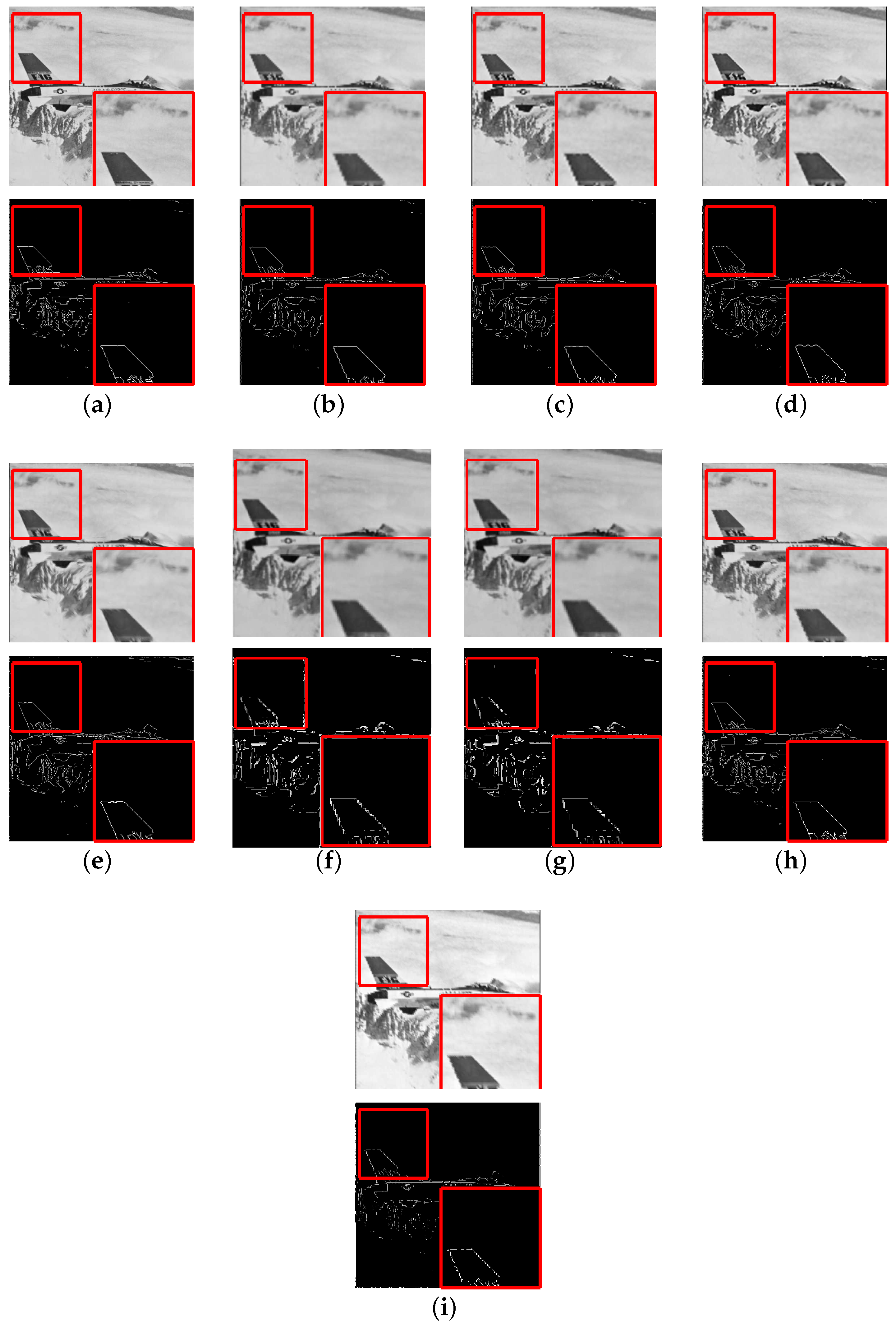
Given a digital gray-scale original image $G(x,y)$ of size $M\times N$, $g_{i,j}(i=0,1,\dots ,M-1;j=0,1,\dots ,N-1)$ is the gray-scale value of the pixel at row i and column j. Any three adjacent pixels of the original image, for example, $g_{i+1,j},g_{i+1,j+1},g_{i,j}$ or $g_{i,+1j},g_{i,j},g_{i+1,j+1},$ constitute a triangular interpolation domain T, marked as $\Delta V_1{V}_2{V}_3$. Note

$$\begin{array}{cc}\hfill \Omega & =\left\{\left(g_{i+1,j},g_{i+1,j+1},g_{i,j}\right)\right|0\le i\le M-1,0\le j\le N-1\}\hfill \\ \hfill & \cup \left\{\left(g_{i,j+1},g_{i,j},g_{i+1,j+1}\right)\right|0\le i\le M-1,0\le j\le N-1\}.\hfill \end{array}$$

(37)

Consider area $\left\{\left.\left(x,y\right)\right|\left(x,y\right)\in \Delta V_1{V}_2{V}_3\right\}$ where $\left(V_1,V_2,V_3\right)\in \Omega$. $V_i$ locates at row $x_i$ and column $y_i$.

According to the side–side method, the constructed Coons patch on $\Delta V_1{V}_2{V}_3$ where $\left(V_1,V_2,V_3\right)\in \Omega$ can be written as follows

$$\begin{array}{c}\hfill f_{\Delta V_1{V}_2{V}_3}\left(\mathrm{x},y\right)={\omega }_1{P}_1\left[F\right]+{\omega }_2{P}_2\left[F\right]+{\omega }_3{P}_3\left[F\right],\end{array}$$

(38)

where $P_i\left[F\right]$ is the same as (6)–(8), $F\left(Q\right)$ is the value of linear interpolation to the original image I at the point Q, $\frac{\partial F}{\partial e_i}(Q)=(x_j-x_k)F_x(e_i)+(y_j-y_k)F_y(e_i),e_i=V_k-V_j$, and alter the first-order partial derivative with difference quotient as follows

$$\begin{array}{c}\hfill F_x(e_i)=\left\{\begin{array}{c}\frac{g_k-g_j}{x_k-x_j},x_k\ne x_j,\\ 0,x_k=x_j,\end{array}\right.\end{array}$$

(39)

$$\begin{array}{c}\hfill F_y(e_i)=\left\{\begin{array}{c}\frac{g_k-g_j}{y_k-y_j},y_k\ne y_j,\\ 0,y_k=y_j.\end{array}\right.\end{array}$$

(40)

According to the side–vertex method, the constructed Coons patch on $\Delta V_1{V}_2{V}_3$ where $\left(V_1,V_2,V_3\right)\in \Omega$ can be written as follows

$$\begin{array}{c}\hfill f_{\Delta V_1{V}_2{V}_3}\left(\mathrm{x},y\right)={\overline{\omega }}_1{D}_1\left[F\right]+{\overline{\omega }}_2{D}_2\left[F\right]+{\overline{\omega }}_3{D}_3\left[F\right],\end{array}$$

(41)

where $D_i\left[F\right]$ is the same as (19), $F\left(Q\right)$ is the value of linear interpolation to the original image I at the point Q, $\frac{\partial F}{\partial e_i}(S_i)=0$, $\frac{\partial F}{\partial e_i}(S_i)=(x_j-x_k)F_x(e_i)+(y_j-y_k)F_y(e_i),e_i=V_k-V_j$ and, alter the partial derivative with difference quotient as (39) and (40).

In fact, (38) and (41) is to obtain linear interpolation function $F(x,y)$ to the input image I, and then construct Coons patch interpolating to $F(x,y)$. The above construction progress shows that the whole interpolated surface $f\left(x,y\right)(0\le x\le M-1,0\le y\le N-1)$ is spliced by $2\times \left(M-1\right)\times \left(N-1\right)$ piecewise Coons patches $f_{\Delta V_1{V}_2{V}_3}\left(\mathrm{x},y\right)$. The interpolation surface $f\left(x,y\right)$ can be written as follows

$$\begin{array}{c}\hfill f(x,y)=f_{\Delta V_1{V}_2{V}_3}\left(\mathrm{x},y\right),when\left(x,y\right)\in \Delta V_1{V}_2{V}_3,\end{array}$$

(42)

where $\left(V_1,V_2,V_3\right)\in \Omega$.

By up-sampling to the constructed interpolation surface $f(x,y)$, a high-resolution image can be obtained.

3. Results

Let $\Delta T$ be the triangle with vertexes $V_1(0,0),V_2(1,0),V_3(0,1)$. Construct Coons patches by SS and SV interpolating to the following function over the triangular domain $\Delta T$, which are shown in Figure 1.

$$\begin{array}{c}\hfill F(x,y)=5.2exp(\frac{-x^2-{(y-0.5)}^2}{4}),\end{array}$$

(43)

Given scattered data generated from (43) on $[0,5]\times [0,5]$, and Delaunay triangulation is shown in Figure 2. Construct two classes of Coons patches over the Delaunay triangulation by SS and SV, which are shown in Figure 3. Theorems 1 and 2 prove that two classes of Coons patches satisfy $C^1$-continuous splice.

To compare the proposed method with bilinear, bicubic, ICBI [22], NEDI [23], SR-NLM [24] and RBC [25], we tested three standard gray-scale images (8-bits, $512\times 512$): ‘pepper’, ‘plane’ and ‘flower’ from BSD200 [30]. The image zooming factor is 4. First, we obtain the low-resolution images down-sampled by the original images with factor 1/4 and then up-sample using SS and SV methods based on the proposed rational quadratic trigonometric Hermite functions with factor 4. The values of shape parameters are listed in

Table 1. Values of shape parameters.

Parameter	${\mathit{\alpha }}_1$	${\mathit{\beta }}_1$	${\mathit{\alpha }}_2$	${\mathit{\beta }}_2$	${\mathit{\alpha }}_3$	${\mathit{\beta }}_3$
$S{S}_1$	1	1	1	1	1	1
$S{V}_1$	1	1	1	1	1	1
$S{S}_2$	0.9	1	2	3	1	4
$S{V}_2$	1	1.01	1	1.06	1	1.05

.

Experimental outcomes are assessed by the well-known state-of-the-art image quality assessment metrics: PSNR, SSIM, FSIM [28] and MS-SSIM [29], which are listed in

Table 2. Comparison of different image zooming methods in terms of peak signal to noise ratio (PSNR).

Image	Bilinear	Bicubic	ICBI	NEDI	SR-NLM	RBC	${\mathit{SS}}_1$	${\mathit{SS}}_2$	${\mathit{SV}}_1$	${\mathit{SV}}_2$
Pepper	$23.06$	$22.70$	$26.82$	$22.69$	$22.79$	$22.98$	$26.75$	$27.05$	$26.24$	$26.25$
Plane	$22.23$	$21.88$	$25.05$	$24.88$	$25.29$	$25.79$	$25.58$	$25.76$	$24.34$	$24.35$
Flower	$25.55$	$25.22$	$29.84$	$28.59$	$28.97$	$29.64$	$29.59$	$29.72$	$28.45$	$28.46$
Average	$23.62$	$23.27$	$27.23$	$25.39$	$25.68$	$26.13$	$27.30$	$27.51$	$26.34$	$26.35$

,

Table 3. Comparison of different image zooming methods in terms of Structural similarity index (SSIM).

Image	Bilinear	Bicubic	ICBI	NEDI	SR-NLM	RBC	${\mathit{SS}}_1$	${\mathit{SS}}_2$	${\mathit{SV}}_1$	${\mathit{SV}}_2$
Pepper	$0.717$	$0.705$	$0.784$	$0.669$	$0.666$	$0.699$	$0.780$	$0.784$	$0.780$	$0.781$
Plane	$0.734$	$0.731$	$0.812$	$0.806$	$0.810$	$0.823$	$0.821$	$0.824$	$0.837$	$0.837$
Flower	$0.806$	$0.801$	$0.884$	$0.789$	$0.797$	$0.812$	$0.891$	$0.892$	$0.864$	$0.864$
Average	$0.752$	$0.746$	$0.827$	$0.803$	$0.806$	$0.829$	$0.831$	$0.833$	$0.827$	$0.827$

,

Table 4. Comparison of different image zooming methods in terms of feature similarity (FSIM).

Image	Bilinear	Bicubic	ICBI	NEDI	SR-NLM	RBC	${\mathit{SS}}_1$	${\mathit{SS}}_2$	${\mathit{SV}}_1$	${\mathit{SV}}_2$
Pepper	$0.875$	$0.876$	$0.932$	$0.958$	$0.963$	$0.970$	$0.934$	$0.935$	$0.937$	$0.937$
Plane	$0.734$	$0.731$	$0.906$	$0.943$	$0.946$	$0.952$	$0.910$	$0.911$	$0.914$	$0.914$
Flower	$0.897$	$0.897$	$0.952$	$0.936$	$0.944$	$0.954$	$0.952$	$0.953$	$0.942$	$0.940$
Average	$0.871$	$0.871$	$0.930$	$0.956$	$0.951$	$0.959$	$0.932$	$0.933$	$0.931$	$0.931$

and

Table 5. Comparison of different image zooming methods in terms of multiscale structural similarity (MS-SSIM).

Image	Bilinear	Bicubic	ICBI	NEDI	SR-NLM	RBC	${\mathit{SS}}_1$	${\mathit{SS}}_2$	${\mathit{SV}}_1$	${\mathit{SV}}_2$
Pepper	$0.836$	$0.836$	$0.899$	$0.869$	$0.876$	$0.881$	$0.903$	$0.905$	$0.908$	$0.908$
Plane	$0.813$	$0.813$	$0.892$	$0.718$	$0.930$	$0.940$	$0.894$	$0.900$	$0.904$	$0.905$
Flower	$0.844$	$0.844$	$0.931$	$0.915$	$0.919$	$0.926$	$0.931$	$0.932$	$0.923$	$0.924$
Average	$0.831$	$0.831$	$0.909$	$0.834$	$0.908$	$0.916$	$0.909$	$0.912$	$0.912$	$0.912$

. The values of PSNR, SSIM, FSIM and MS-SSIM of NEDI, SR-NLM and RBC are referenced from [25].

For visual quality assessment and edge detection, Figure 4 and Figure 5 show the pepper and plane images up-scaled by eight methods: bilinear, bicubic, ICBI, NEDI, SR-NLM, RBC and the proposed SS and SV methods. The image zooming results of SR-NLM and RBC are downloaded from [25]. For sensitivity analysis of SS and SV, Figure 6 and Figure 7 show PSNR, SSIM, FSIM and MS-SSIM tested on the image zooming results with $r=\frac{{\alpha }_1}{{\beta }_1}=\frac{{\alpha }_2}{{\beta }_2}=\frac{{\alpha }_3}{{\beta }_3},r\in \left(0,4\right]$.

4. Discussion

In Figure 1, for SS and SV, both the interior Coons patches shows convex shape when $\alpha <\beta$ and concave shape when $\alpha >\beta$. When $\alpha =\beta$, it shows convex interior shape in the middle for SS and concave interior shape for SV. However, Coons patches constructed by the proposed methods always interpolate to function value and the first partial derivative on the boundary.

In Figure 3, it is shown that when changing the values of shape parameters, Coons patches splice shows piecewise convex or concave, so as to achieve the complex surface design. Splice of Coons patches constructed by the proposed methods always keep $C^1$-continuity at the boundary of the piecewise Coons patch.

In Table 2, Table 3, Table 4 and Table 5, $S{S}_1$ and $S{S}_2$ has the highest PSNR values on aveage, and have slightly lower FSIM and MS-SSIM values than SR-NLM and RBC. $S{S}_2$ has the highest SSIM values on average. $S{S}_2$ have higher PSNR, SSIM and FSIM values than $S{S}_1$, which demonstrates that we can acquire higher quality images by adjusting values of shape parameters. $S{V}_1$ and $S{V}_2$ have similar indexes, for values of shape parameters are close. $S{V}_1$ and $S{V}_2$ have higher MS-SSIM values than bilinear, bicubic, ICBI, NEDI, SR-NLM, $S{S}_1$ and $S{S}_2$ on average. Therefore, our methods still give pleasing results overall.

For visual quality assessment, in Figure 4, we find that SR-NLM and RBC lose edge details, while bilinear, bicubic, ICBI, NEDI, SS and SV preserve clear edges. In Figure 5, we find that bilinear, SR-NLM, RBC, SS and SV preserve sharp and straight edges in the highlighted area, while deformed edges are detected in bicubic, ICBI and NEDI. Bilinear, bicubic and ICBI show the problem of damaging the texture on other areas (e.g., The mountain of the plane image), where the edge detections show circle textures instead of complex textures. Compared to SR-NLM and RBC, SS and SV have sharper edges in the highlighted area and clearer texture details in another area (e.g., The mountain of the plane image). More texture details were detected in SS than SV.

Through computation, we find that SS with ${\alpha }_1=0.9,{\beta }_1=1,{\alpha }_2=2,{\beta }_2=3,{\alpha }_3=1,{\beta }_3=4$ ($S{S}_2$) and SV with ${\alpha }_1=1,{\beta }_1=1.01,{\alpha }_2=1,{\beta }_2=1.06,{\alpha }_3=1,{\beta }_3=1.05$ ($S{V}_2$) will give best image zooming results.

For sensitivity analysis, from Figure 6 and Figure 7, we find that for SS, indexes values of image zooming quality are sensitive to values of shape parameters when $r=\frac{{\alpha }_1}{{\beta }_1}=\frac{{\alpha }_2}{{\beta }_2}=\frac{{\alpha }_3}{{\beta }_3}\in \left(0,1\right]$, and indexes values maintain high when $r\in \left[1,4\right]$. For SV, indexes values are sensitive to values of shape parameters, and it achieve the highest quality when r is around 1.

In conclusion, in order to improve the quality of image zooming, we proposed a class of rational quadratic trigonometric Hermite functions with two shape parameters. Based on the proposed functions, using the improved side–side method and side–vertex method for interpolation, we proposed two classes of $C^1$-continuous Coons patches constructions over the triangular domain. Coons patches constructed by the proposed methods always interpolate to the function values and the first-order partial derivatives on the boundary. We can adjust the interior shape of Coons patches by altering the values of shape parameters without influencing the boundary shape. Splice of $C^1$-continuous Coons patches constructed by the proposed methods can interpolate to complex surface. Since the Coons patches are constructed over the triangular domain, they can interpolate to scattered data through the Delaunay triangulation.

Applying the proposed Coons patches construction to image zooming, we give region control of shape parameters to deal with the problem of well-posedness. We also give sensitivity analysis on values of shape parameters. Compared to bilinear, bicubic, ICBI, NEDI, SR-NLM and RBC, the proposed methods improve PSNR and SSIM. Through edge detection analysis by Prewitt operator, compared to these six methods, the proposed methods can better preserve sharp edges and textures. Therefore the proposed Coons patch construction can improve the visual effect of the image and it is effective in computation for image zooming. Our future work will be $C^2$-continuous Coons surfaces over the triangular domain with shape parameters.

References

1. Gonzalez, R.C.; Woods, R.E. Image Enhancement in the spatial Domain. In Digital Image Processing; Dworkin, A., Ed.; Prentice Hall: New York, NY, USA, 2002; pp. 76–142. [Google Scholar]
2. Keys, R.G. Cubic convolution interpolation for digitalimage processing. IEEE Trans. Acoust. Speech Signal Process. 1981, 29, 1153–1160. [Google Scholar] [CrossRef] [Green Version]
3. Park, S.K.; Schowengerdt, R.A. Image reconstruction by parametric cubic convolution. Comput. Vis. Graph. Image Process. 1983, 23, 258–272. [Google Scholar] [CrossRef]
4. Lehmann, T.M.; Gonner, C.; Spitzer, K. Survey: Interpolation methods in medical image processing. IEEE Trans. Med. Imaging 2000, 18, 1049–1075. [Google Scholar] [CrossRef] [PubMed] [Green Version]
5. Muresan, D.D.; Parks, T.W. Adaptively quadratic (AQua) image interpolation. IEEE Trans. Image Process. 2004, 13, 690–698. [Google Scholar] [CrossRef]
6. Han, P.; Su, Z.; Liu, X. Image interpolation using Coons surface patch with shape control parameters. J. Comput.-Aided Des. Comput. Graph. 2005, 17, 976–980. [Google Scholar]
7. Li, J.; Zhao, D.; Lu, Y. Image Zooming Using Rational Coons Interpolation patch with shape Parameters. J. Comput.-Aided Des. Comput. Graph. 2011, 23, 1853–1859. [Google Scholar]
8. Barnhill, R.E.; Birkhoff, G.; Gordon, W.J. Smooth interpolation in triangles. J. Approx. Theory 1973, 8, 114–128. [Google Scholar] [CrossRef] [Green Version]
9. Barnhill, R.E.; Gregory, J.A. Compatible smooth interpolation in triangles. J. Approx. Theory 1975, 15, 214–225. [Google Scholar] [CrossRef] [Green Version]
10. Barnhill, R.E.; Gregory, J.A. Polynomial interpolation to boundary data on triangle. Math. Comput. 1975, 29, 726–735. [Google Scholar] [CrossRef]
11. Gregory, J.A. Smooth interpolation without twist constraints. In Computer Aided Geometric Design; Barnhill, R.E., Resenfeld, R.F., Eds.; Academic Press: New York, NY, USA, 1974; pp. 71–88. [Google Scholar]
12. Gregory, J.A. A blending function interpolant for triangles. In Multivariate Approximation; Handscomb, D.C., Ed.; Academic Press: New York, NY, USA, 1978; pp. 279–287. [Google Scholar]
13. Gregory, J.A. C1 rectangular and nonrectangular surface patches. In Surfaces in Computer Aided Geometric Design; Barnhill, R.E., Boehm, W., Eds.; North-Holland: Amsterdam, The Netherlands, 1983; pp. 25–33. [Google Scholar]
14. Nielson, G.M. The side vertex method for interpolation in triangles. J. Approx. Theory 1979, 25, 318–336. [Google Scholar] [CrossRef] [Green Version]
15. Hagen, H. Geometric surface patches without twist constraints. Comput. Aided Geom. Des. 1986, 3, 179–184. [Google Scholar] [CrossRef]
16. Hagen, H. Curvature continuous triangular interpolants. In Methods in CAGD; Lyche, T., Schumaker, L., Eds.; Academic Press: Oslo, Norway, 1989; pp. 373–384. [Google Scholar]
17. Nielson, G.M. A transfinite, visually continuous, triangular interpolant. In Geometric Modeling, Applications and New Trends; Farin, G., Ed.; SIAM: Philadelphia, PA, USA, 1987; pp. 235–246. [Google Scholar]
18. Tang, Y.; Wu, X.; Han, X. C1-Continuous H-Type Coons Patches on Triangles. J. Eng. Graph. 2010, 31, 97–103. [Google Scholar]
19. Wu, X.; Han, X.; Luo, S. C1-Continuous triangular Coons Patches with shape parameters. Comput. Appl. 2008, 28, 3123–3125. [Google Scholar]
20. Wu, X.; Han, X.; Luo, S.; Wang, J. C1-Continuous C-Type Coons Patches on Triangles. Appl. Res. Comput. 2009, 26, 1538–1540. [Google Scholar]
21. Wu, X.; Han, X.; Tang, Y. C1-Continuous T-Type Coons Patches on Triangles. Comput. Eng. Appl. 2010, 46, 173–176. [Google Scholar]
22. Giachetti, A.; Asuni, N. Real-time artifact-free image upscaling. IEEE Trans. Image Process. 2011, 20, 1538–1540. [Google Scholar] [CrossRef]
23. Li, X.; Orchard, M.T. New edge-directed interpolation. IEEE Trans Image Process. 2001, 10, 1521–1527. [Google Scholar]
24. Hung, K.W.; Siu, W.C. Single-image super-resolution using iterative Wiener filter based on nonlocal means. Signal Process. Image Commun. 2015, 39, 26–45. [Google Scholar] [CrossRef]
25. Abbas, S.; Hussain, M.Z.; Irshad, M. Image interpolation by rational ball cubic B-spline representation and genetic algorithm. Alex. Eng. J. 2017, 57, 931–937. [Google Scholar] [CrossRef]
26. Coons, S.A. Surfaces in Computer-Aided Design of Space Forms; Technical report MAC-TR-41; MIT: Cambridge, MA, USA, 1967. [Google Scholar]
27. Zhu, Y.P. C2 positivity-preserving rational interpolation splines in one and two dimensions. Appl. Math. Comput. 2018, 316, 186–204. [Google Scholar] [CrossRef]
28. Zhang, L.; Zhang, L.; Mou, X.Q.; Zhang, D. FSIM: A Feature Similarity Index for Image Quality Assessment. IEEE Trans. Image Process. 2011, 20, 2378–2386. [Google Scholar] [CrossRef] [PubMed] [Green Version]
29. Wang, Z.; Simoncelli, E.; Bovik, A. Multiscale structural similarity for image quality assessment. In Proceedings of the Thrity-Seventh Asilomar Conference on Signals, Systems & Computers, Pacific Grove, CA, USA, 9–12 November 2003; Volume 2, pp. 1398–1402. [Google Scholar]
30. Martin, D.; Fowlkes, C.; Tal, D.; Malik, J. A Database of Human Segmented Natural Images and its Application to Evaluating Segmentation Algorithms and Measuring Ecological Statistics. In Proceedings of the Eighth IEEE International Conference on Computer Vision (ICCV 2001), Vancouver, BC, Canada, 7–14 July 2001; Volume 2, pp. 416–423. [Google Scholar]
Figure 1. Coons patches constructed by SS and SV. (a) SS with α 1 = β 1 = α 2 = β 2 = α 3 = β 3 = 1 . (b) SS with α 1 = α 2 = α 3 = 1 , β 1 = 10 , β 2 = 15 , β 3 = 20 . (c) SS with α 1 = 10 , α 2 = 15 , α 3 = 20 , β 1 = β 2 = β 3 = 1 . (d) SV with α 1 = β 1 = α 2 = β 2 = α 3 = β 3 = 1 . (e) SV with α 1 = α 2 = α 3 = 1 , β 1 = 1 . 1 , β 2 = 1 . 2 , β 3 = 1 . 3 . (f) S with α 1 = 1 . 1 , α 2 = 1 . 2 , α 3 = 1 . 3 , β 1 = β 2 = β 3 = 1 .
Symmetry 12 00661 g001
Figure 2. Delaunay triangulation of the scattered data.
Symmetry 12 00661 g002
Figure 3. Splice of Coons patches constructed by side–side (SS) and side–vertex (SV). (a) SS with α 1 = β 1 = α 2 = β 2 = α 3 = β 3 = 1 . (b) SS with α 1 = α 2 = α 3 = 1 , β 1 = 10 , β 2 = 15 , β 3 = 20 . (c) SS with α 1 = 10 , α 2 = 15 , α 3 = 20 , β 1 = β 2 = β 3 = 1 . (d) SV with α 1 = β 1 = α 2 = β 2 = α 3 = β 3 = 1 . (e) SV with α 1 = α 2 = α 3 = 1 , β 1 = 10 , β 2 = 13 , β 3 = 1 . 2 . (f) SV with α 1 = 10 , α 2 = 13 , α 3 = 1 . 2 , β 1 = β 2 = β 3 = 1 .
Symmetry 12 00661 g003
Figure 4. Image zooming and edge detection results on image ‘pepper’ by different algorithm (Factor 4). (a) Original. (b) Bilinear. (c) Bicubic. (d) Iterative curvature-based interpolation (ICBI). (e) Novel edge orientation adaptive interpolation scheme for resolution enhancement of still images (NEDI). (f) Super-resolution using iterative Wiener filter based on nonlocal means (SR-NLM). (g) Rational ball cubic B-spline (RBC). (h) SS with α 1 = 0 . 9 , β 1 = 1 , α 2 = 2 , β 2 = 3 , α 3 = 1 , β 3 = 4 . (i) SV with α 1 = 1 , β 1 = 1 . 01 , α 2 = 1 , β 2 = 1 . 06 , α 3 = 1 , β 3 = 1 . 05 .
Symmetry 12 00661 g004
Figure 5. Image zooming and edge detection results on image ‘plane’ by different algorithm (Factor 4). (a) Original. (b) Bilinear. (c) Bicubic. (d) ICBI. (e) NEDI. (f) SR-NLM. (g) RBC. (h) SS with α 1 = 0 . 9 , β 1 = 1 , α 2 = 2 , β 2 = 3 , α 3 = 1 , β 3 = 4 . (i) SV with α 1 = 1 , β 1 = 1 . 01 , α 2 = 1 , β 2 = 1 . 06 , α 3 = 1 , β 3 = 1 . 05 .
Symmetry 12 00661 g005
Figure 6. Sensitivity analysis of SS with r = α 1 β 1 = α 2 β 2 = α 3 β 3 (Factor 4). (a) Peak signal to noise ratio (PSNR). (b) Structural similarity (SSIM). (c) Feature similarity (FSIM). (d) Multiscale structural similarity (MS-SSIM).
Symmetry 12 00661 g006
Figure 7. Sensitivity analysis of SV with r = α 1 β 1 = α 2 β 2 = α 3 β 3 (Factor 4). (a) PSNR. (b) SSIM. (c) FSIM. (d) MS-SSIM.
Symmetry 12 00661 g007