A Fast UTD-Based Method for the Analysis of Multiple Acoustic Diffraction over a Series of Obstacles with Arbitrary Modeling, Height and Spacing

Abstract

A uniform theory of diffraction (UTD)-based method for analysis of the multiple diffraction of acoustic waves when considering a series of symmetric obstacles with arbitrary modeling, height and spacing is hereby presented. The method, which makes use of graph theory, funicular polygons and Fresnel ellipsoids, proposes a novel approach by which only the relevant obstacles and paths of the scenario under study are considered, therefore simultaneously providing fast and accurate prediction of sound attenuation. The obstacles can be modeled either as knife edges, wedges, wide barriers or cylinders, with some other polygonal diffracting elements, such as doubly inclined, T- or Y-shaped barriers, also considered. In view of the obtained results, this method shows good agreement with previously published formulations and measurements whilst offering better computational efficiency, thus allowing for the consideration of a large number of obstacles.

1. Introduction

Different approaches have been carried out for the analysis of the acoustic wave diffraction caused by multiple obstacles. These approaches are typically based on boundary element methods (BEMs) [1], parabolic equation methods [2], the geometrical/uniform theory of diffraction (GTD/UTD) [3,4,5,6,7,8] or empirical formulae [9]. Among such methods, the GTD/UTD offers reduced mathematical complexity by entirely explaining the problem of wave diffraction in terms of rays, thereby considerably shortening the computation time.

Keller published the GTD [10] about 60 years ago and it is accurate for most practical cases providing that the sound wavelength is smaller than the obstacle dimensions. However, this theory fails in the vicinity of shadow boundaries (e.g., when the source, obstacle and receiver lie within a straight line). This shortcoming was later solved by Kouyoumjian and Pathak [11] by the proposal of the UTD, whose formulation is also applicable at shadow and reflection boundaries. This formulation allows for the multiple diffraction of acoustic waves in such environments where a set of identical diffracting obstacles are evenly spaced and can be of special relevance (e.g., the rows of seats in common auditoriums or concert halls). In this sense, some of the authors of this study have recently published works [7,8] where two-dimensional (2D) UTD formulations for such types of environments have been presented.

On the other hand, the analysis of the acoustic diffraction caused by obstacles of arbitrary height and spacing can also be of great importance in many practical applications. In this sense, Pierce developed an asymptotic solution to solve the diffraction around a wedge or a wide barrier, which is based on the concepts of GTD [3], as well as an exact formulation together with Hadden for sound diffraction over screens and wedges [12]. Later, Kawai proposed a GTD/UTD solution based on Pierce’s formulation for the analysis of sound diffraction by a many-sided barrier or pillar [4]. Kim et al. presented a GTD-based solution for the study of multiple acoustic diffraction caused by multiple wedges, barriers and polygonal-like shapes [5]. Finally, Min and Qiu proposed a GTD method for analyzing sound diffraction around rigid, parallel, wide barriers [6].

Nevertheless, the main limitation of the above-mentioned works lies in the highly demanding computing requirements when a large number of obstacles is to be analyzed. Moreover, despite the widely different approaches and studies on multiple acoustic diffraction, to the best of the authors’ knowledge, there is not yet an accurate and general solution for multiple sound diffraction that can take into consideration obstacles with arbitrary modeling, height and spacing.

In this paper, contrary to previous works of the authors [7,8] where only acoustic multiple-diffraction over obstacles of equal shape, height and spacing was analyzed, an innovative UTD-based method for the analysis of the multiple diffraction of acoustic waves when considering a series of symmetric obstacles with arbitrary modeling, height and spacing is presented. This way, the scenario considered in previous studies published by the authors not only is extended in terms of the possible shape, height and location of the obstacles (that is, in this work, those parameters can vary from one obstacle to another within the same array) but also the analysis is carried out from a fully different approach. In this sense, the formulations presented in [7] and [8] were based on radio wave recursive relations emerging from the application of both UTD and physical optics (PO) theories. However, the method hereby presented is a pure-UTD acoustic approach which makes use of graph theory, funicular polygons and Fresnel ellipsoids, so that only the relevant obstacles and paths of a complex scenario are considered, therefore providing a fast, computationally efficient—while at the same time accurate—prediction of sound attenuation. On this basis, a great number of obstacles (including neighboring ones of equal height) can be analyzed in an acceptable time and such obstacles can be modeled either as knife edges, wedges, wide barriers or cylinders, as well as some other polygonal diffracting elements, such as T- or Y-shaped barriers.

2. Theoretical Method

The theoretical method proposed in this work is a UTD ray-based solution developed to analyze multiple acoustic diffraction (and also reflections) of spherical waves in scenarios, which can include parallel wide barriers, screens (knife edges), wedges, cylinders and polygonal shapes, such as T or Y barriers. An example of such a configuration can be observed in Figure 1.

The method is 2D, for which all these obstacles are assumed to be infinitely long. Moreover, the first-order diffracted field of the rays will be considered, as well as perfectly reflecting (ρ = 1) (acoustically hard) materials. However, the proposed method can be easily extended for specific input impedances, since the reflection coefficients as a function of the frequency are well known.

As a result, the total diffracted (and reflected on the floor/ground) complex pressure field at the receiver R from a source S will be the summation of the overall rays impinging on R and coming from all the possible paths [10,11]:

$${\varphi }_t{}_{Rx}={\displaystyle {\displaystyle \sum }_{i=1}^n}{\varphi }_i\left(S,R\right)$$

(1)

where ${\varphi }_i\left(S,R\right)$ is the complex received field of an individual ray from the source S to the receiver R following one of the selected n possible paths. S is assumed as a point source which generates a spherical wave front within an ideal isotropic (uniform) medium such as air, whereas the receiver (R) of the acoustic field would be a listener with an isotropic pattern having unity gain. The phase is taken into consideration for each signal traversing each path, taking advantage of the GTD/UTD theory that combines the representation of rays with the diffraction phenomenon, thereby allowing the calculation of the field at the receiver as the vector resulting from the addition of the fields corresponding to each ray.

2.1. Selection of Nodes of the Scenario

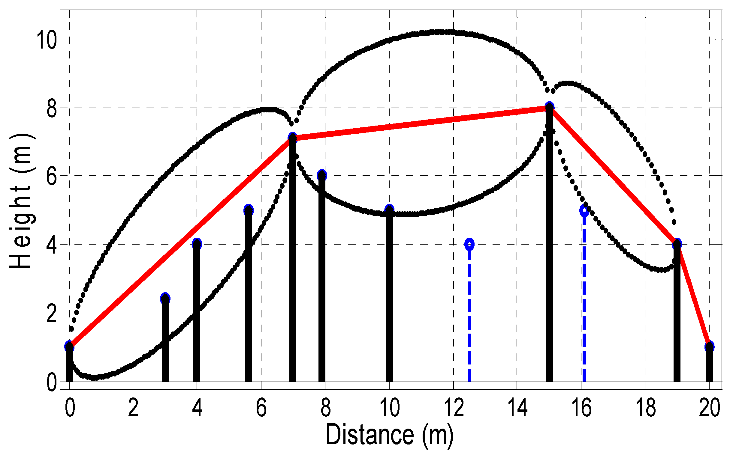
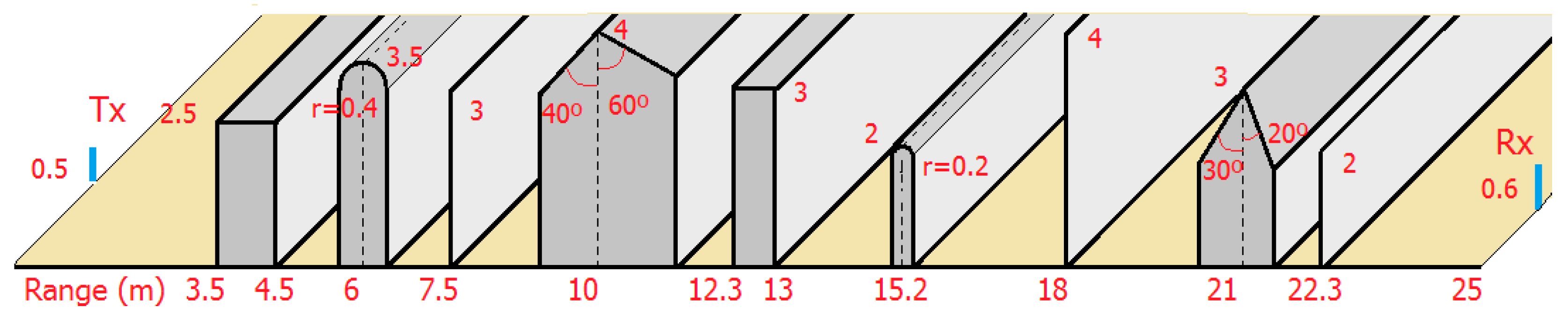
In the first stage of the method, the profile under research is entered by defining the heights, spacing, type or shape of each obstacle (e.g., knife edge, wedge, cylinder, wide-barrier or polygonal element) as well as the parameters corresponding to the type of obstacle, if applicable (e.g., interior angles for wedges, radii for cylinders or widths for wide barriers).

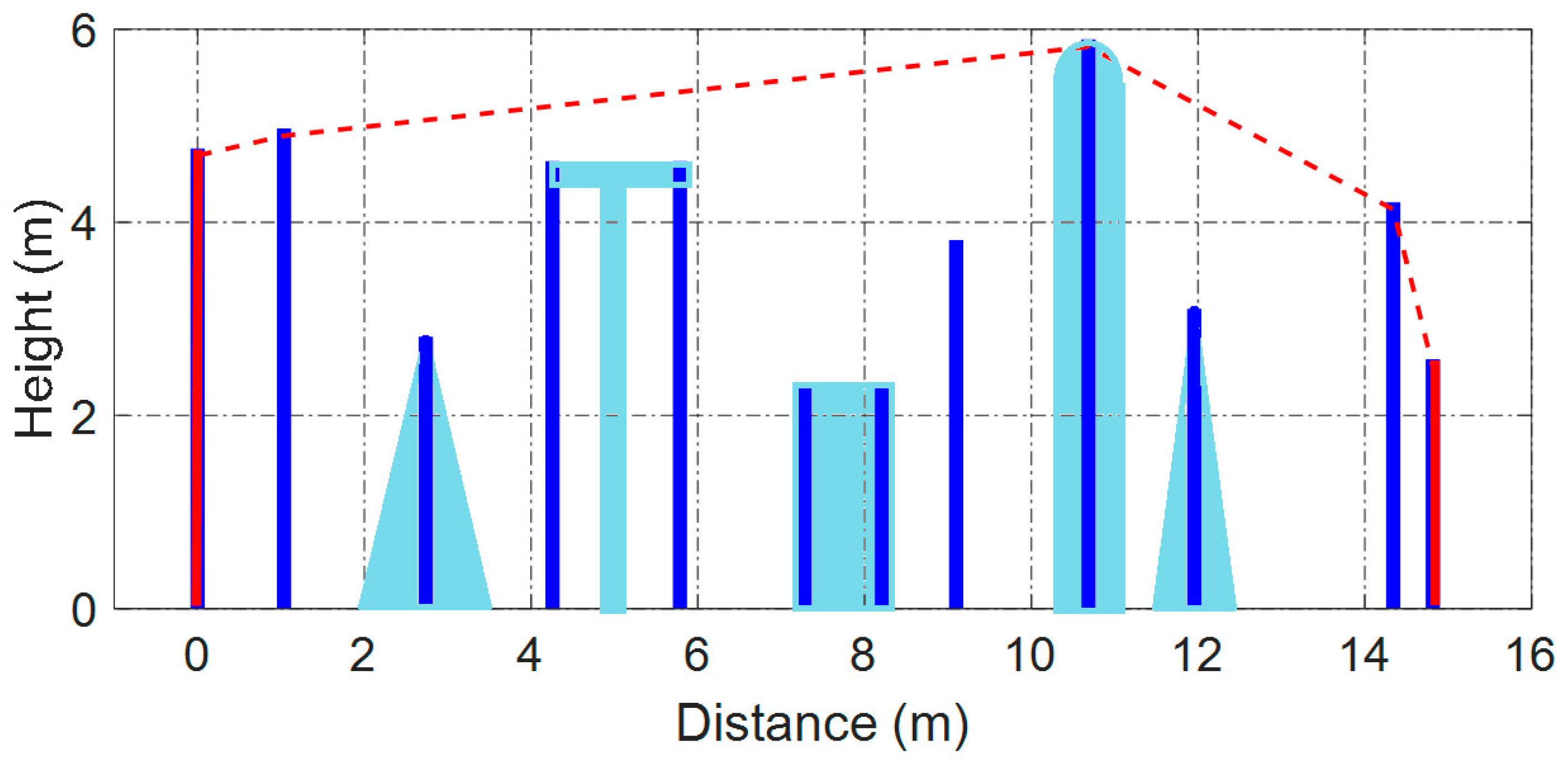
For this purpose, firstly, it is then required to identify the initial ‘nodes’ taking part of the arbitrary profile, starting from the source up to the receiver. This task is undertaken from the definition of the scenario itself due to the fact that each obstacle can be really composed by either single (knife edges, wedges, cylinders) or connected nodes (wide barriers, T- and Y-shaped, doubly inclined). In order to illustrate the theoretical method, the example shown in Figure 2 will be considered, where a series of different obstacles are present. Specifically, three knife edges, one T-shaped obstacle, one wide barrier, two wedges and one cylinder. The interior angles of the wedges are 20° (wedge on the left) and 10° (wedge on the right). The radius of the cylinder is 0.2 m. The source and the receiver appear in red in the profile.

The same process could be followed with any other scenario, either simpler or more complex. The difference would be the processing time required to get the global complex pressure field received by the listener, which is further discussed in Section 3. What is more, even complex, irregular obstacles could be built by a combination of the said basic shapes within a certain frequency range, although this will not be addressed in the present work.

2.1.1. Case of Knife Edges and Wide Barriers

Most of the typical obstacles that can be present in acoustic applications can be built by properly combining the basic shapes referred to above (wedges or cylinders) and by applying the right diffraction coefficients at both sides of the barrier. By considering this premise, other more complex structures, such as polygonal barriers, were also considered in this work, such as doubly inclined, Y- or T-shaped barriers.

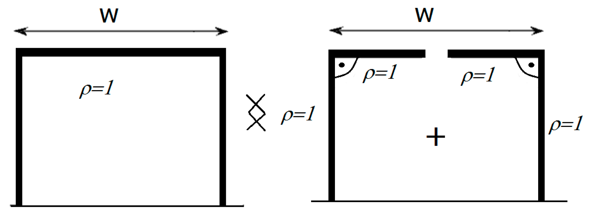
On this basis, wide barriers can be just considered as two joined (interconnected) wedges of interior angle π/2 rad (Figure 3). To take into account the two aligned interconnected edges, a factor of 0.5 in the diffraction coefficient will be applied, as later explained in Section 2.1.2.

Moreover, it should be noted that a knife edge is only a specific case of wedge where the inner angle between the two faces is 0°.

2.1.2. Case of Polygonal T-Shaped Barriers

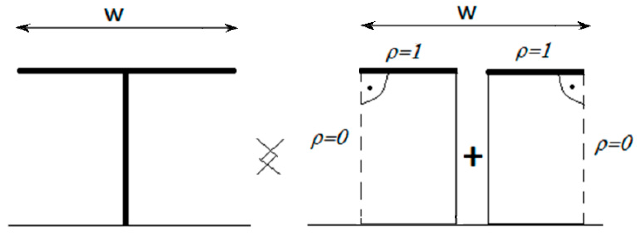
A T-shaped barrier can be successfully constructed by joining two wedges of interior angle π/2 rad with a virtual perfectly absorbing face (ρ = 0) interlaced by a thin screen, as shown in Figure 4, and by applying a factor of 0.5 to account for the two aligned interconnected edges.

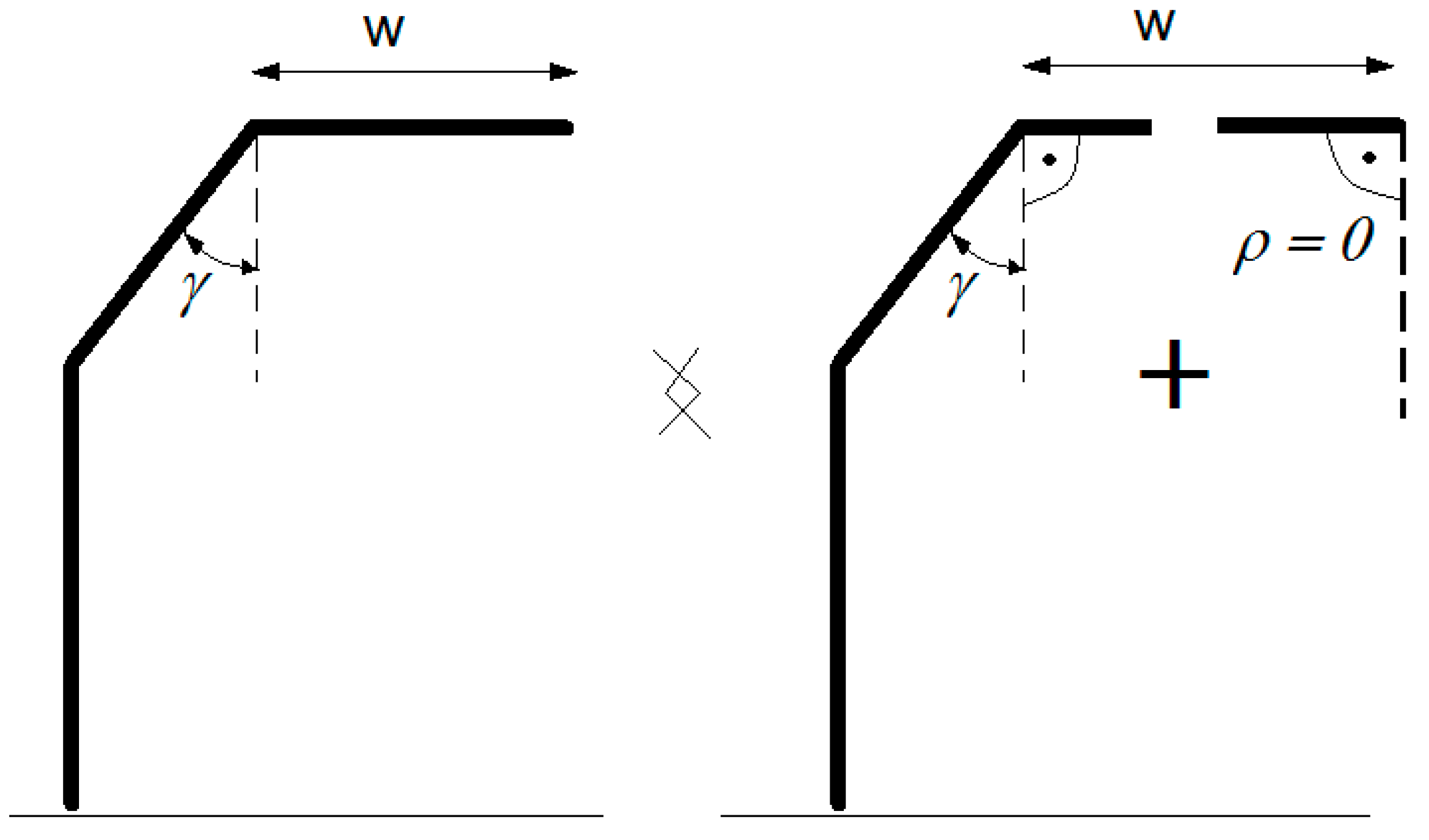
2.1.3. Case of Y-Shaped Barriers

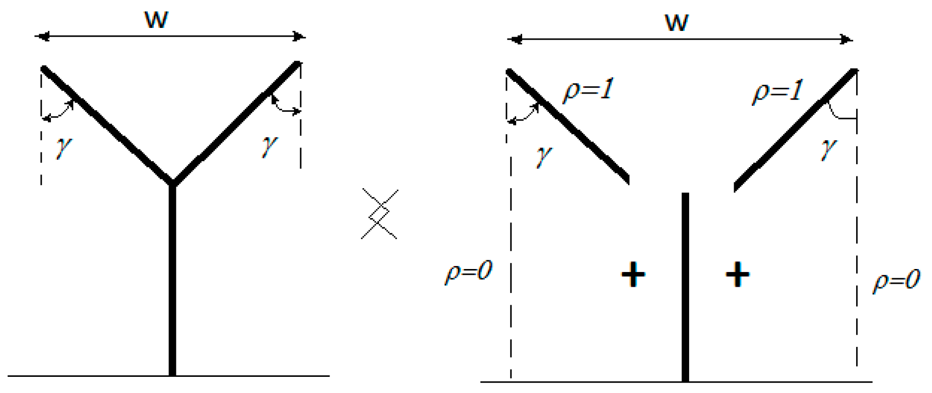
In a similar manner, the Y-shaped barrier can also be modeled, as shown in Figure 5.

The barrier can be seen as two wedges of interior angle γ rad with a perfectly absorbing face (ρ = 0) interlaced by a thin screen.

2.1.4. Case of Doubly Inclined Barriers

Doubly inclined barriers can also be formally considered like wide barriers where their faces can have a certain angle higher than the right-angled one. For the barrier of Figure 6, the face on the right would be equivalent to a perfectly absorbing face (ρ = 0), as previously done for T- or Y-shaped barriers:

2.2. Selection of Relevant Paths and Obstacles

2.2.1. Funicular Profiles

It is then essential, once the extraction of nodes has concluded, to analyze and select only the different paths that are actually contributing to the final sound pressure field at the receiver. In this sense, it is also a key matter to distinguish the obstacles that must be considered in the final profile—and those which can be neglected—depending on if they have a relevant impact (or not) on the total losses. On this basis, an optimum profile in terms of relevant paths and obstacles will result in a much lower computation time without any loss of accuracy in the predicted field at the receiver. For that purpose, a funicular profile (envelope) formed by the successive line of sights (LOS), which can be traced considering the most prominent obstacles that would be part of any path from the source to the receiver, is calculated. For this task, the algorithm iteratively looks for the maximum slope (tangent) among the family of straight lines from the source to any other node of the profile. Once the first node is found, the process is repeated by iteratively shifting the source to the next funicular node, until the receiver is reached.

If we consider the arbitrary profile of Figure 7 extracting the obstacle nodes from the scenario in Figure 2 of different heights and spacing (where the red vertical lines are assumed to be the transmitter and receiver) we can see how five nodes take part in the funicular profile, including the mentioned transmitter and the receiver. The same process would be followed with any other created profile once the nodes are identified.

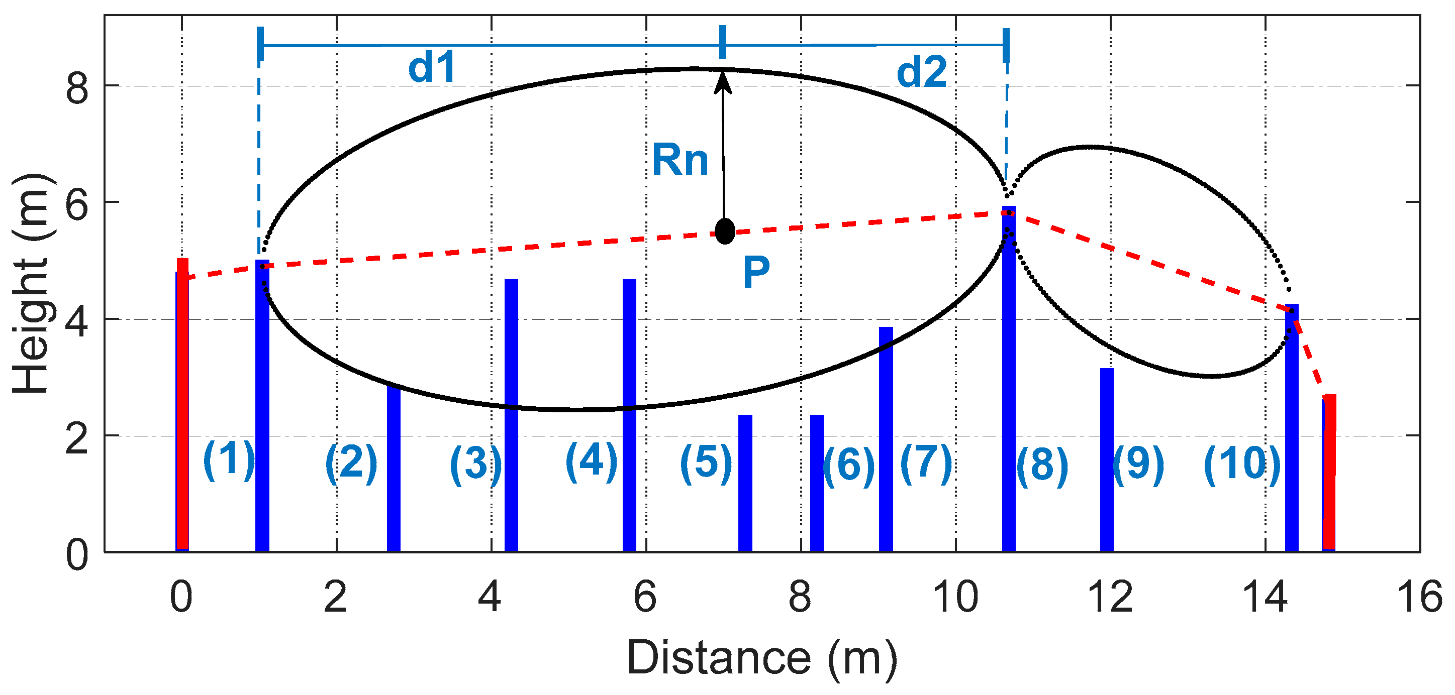
2.2.2. Relevant Obstacles by Fresnel Ellipsoid Method

Once the funicular obstacles (which are common nodes for any path) are identified, the proposed algorithm selects, for each hop that can be formed by two consecutive funicular nodes, the obstacles existing between them that are relevant in the sense of having an impact in terms of loss on the signal strength. In this respect, an obstacle is considered as relevant if it enters the Fresnel zone associated with the ray existing between the two nodes (it will block a significant percentage of energy of the transmitted signal). If the clearance of the Fresnel ellipsoid between two adjacent funicular nodes remains unobstructed with respect to the height of one intermediate obstacle, such an obstacle will be discarded for diffraction loss calculation purposes. As a result, the radius of the Fresnel zone at any point P of the funicular imaginary line (red dashed line in Figure 8) in between the endpoints of any link can be calculated as:

$$R_n=\sqrt{\frac{n·\lambda ·d_1·d_2}{d_1+d_2}}$$

(2)

where λ is the wavelength of the signal, n is the order of the Fresnel zone (1, 2, 3 and so on), d₁ is the distance of any point P from one end of the link and d₂ is the distance of P from the other end, as shown in Figure 8. Equation (2) is derived from the application of the Huygens–Fresnel principle to wave propagation analysis [13], and it characterizes the effective ellipsoid shape, with a maximum radius at the midpoint of the path.

As can be seen in Figure 8 and Figure 9 (where n = 1 and a minimum frequency of 100 Hz is considered), the obstacles 3, 4 and 7 of the example profile enter the Fresnel zone, for which they are considered as relevant obstacles. On the contrary, the obstacles 2, 5, 6 and 9 are initially discarded, as they are out of the Fresnel ellipsoids for the lowest frequency of the analysis.

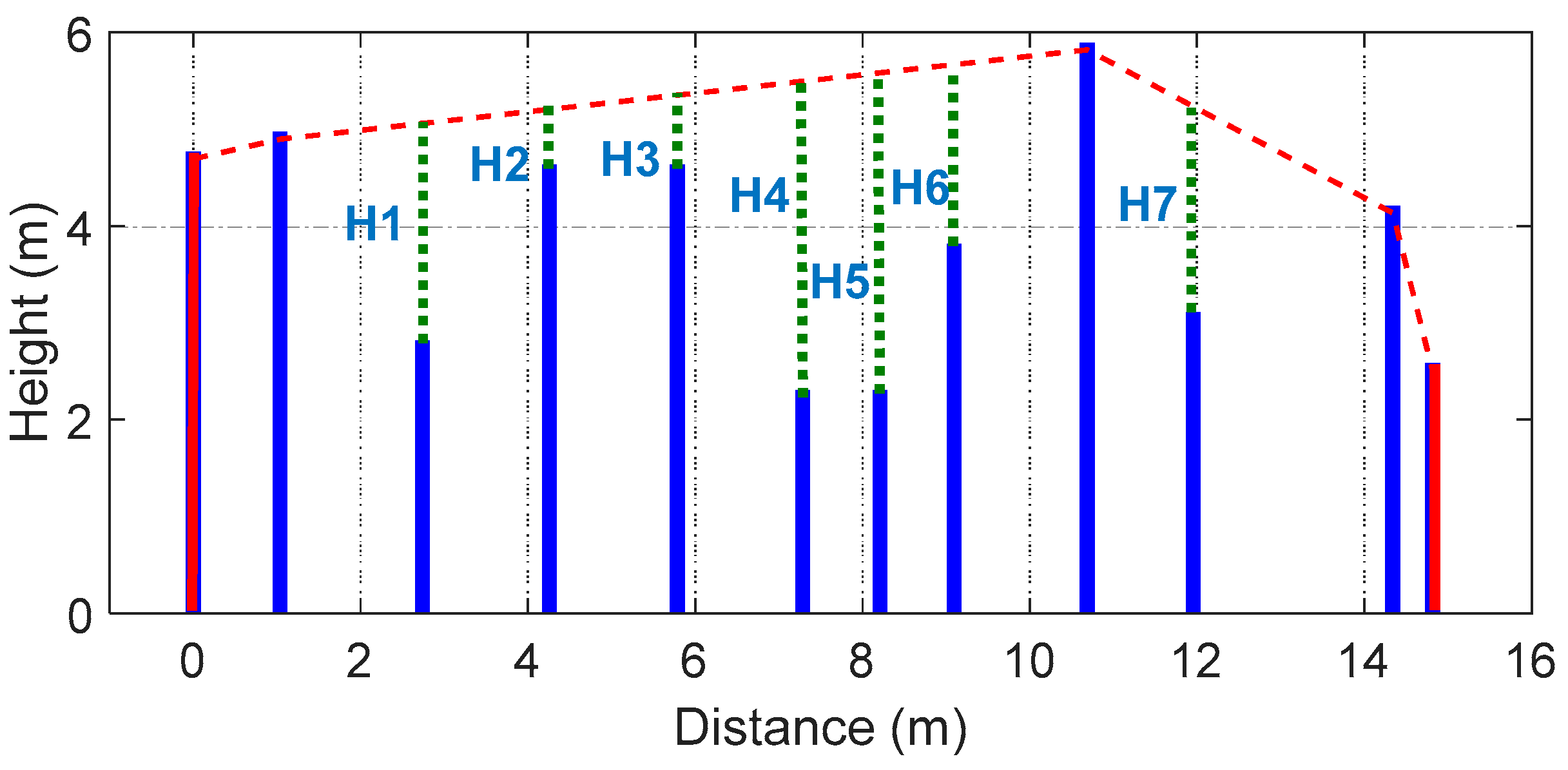
Since the radius of the Fresnel ellipsoid decreases with frequency, additional obstacles can be ignored at higher frequencies (if the frequency band under analysis is wide). In this respect, all the clearances are firstly calculated in the proposed method in order to know the frequencies at which obstacles can be progressively discarded depending on the radius of the corresponding Fresnel zone, so that the optimum computation time to provide the insertion losses (IL) can be achieved, as shown in Figure 9 and Equations (3)–(5):

$$H_i=FunicularHeight-ObstacleHeigh{t}_i$$

(3)

$$H_i=R_1=\sqrt{\frac{1·\lambda d_{1i}·d_{2i}}{d_{1i}+d_{2i}}}$$

(4)

$${\lambda }_i=\frac{H_i{}^2\left(d_{1i}+d_{2i}\right)}{d_{1i}·d_{2i}}$$

(5)

where d_1i and d_2i are the distances to the obstacle node located on the left and on the right of the funicular profile, respectively. Following this step, the method assesses whether the frequency is within the frequency range to be analyzed or not.

In this sense, the obstacle node 7 in the example (Figure 8) will be discarded at frequencies higher than 123.6 Hz. On the contrary, a more conservative but computationally more inefficient method would only evaluate the minimum frequency.

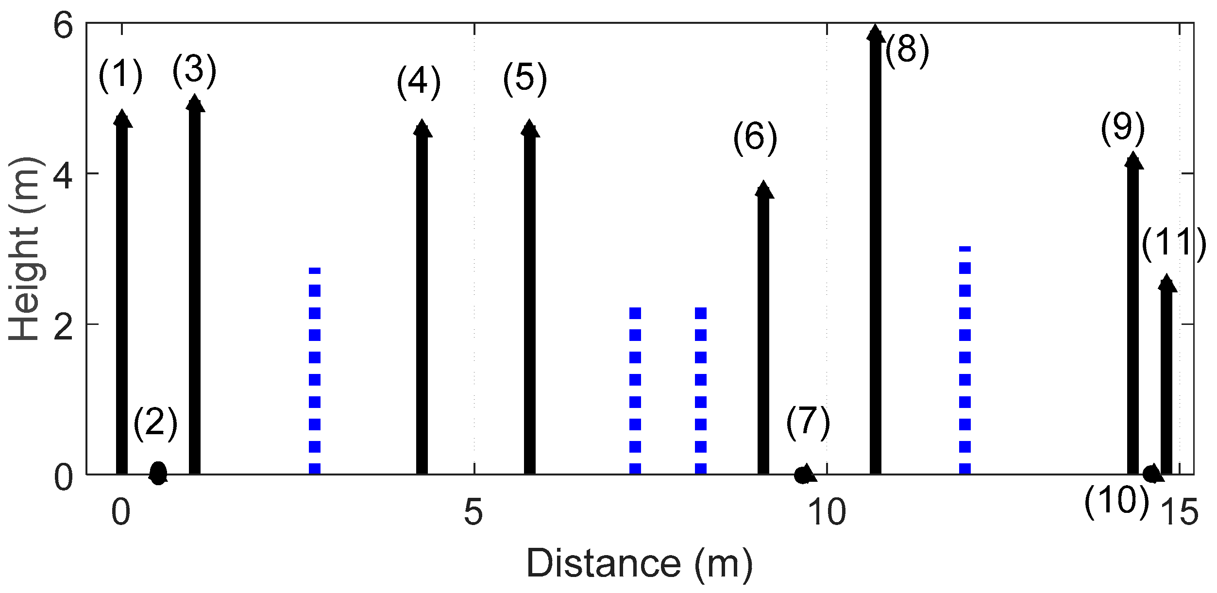
The reflections from the ground can also be calculated and included in the algorithm, so that they can be treated as nodes of the whole profile. As part of the selection process of the relevant obstacles between adjacent funicular nodes, the algorithm could also ignore the reflection points located beside discarded obstacles, since the concerned ray impinging on that point could not reach the receiver unless diffracting over discarded obstacles. On the contrary, the reflection points located between relevant obstacles will be considered. On this basis, in Figure 10, the selection of relevant obstacle nodes and reflection points of the example profile of Figure 2 at 100 Hz can be observed. The selection of final nodes should be renumbered accordingly in case of enabling ground reflection, in order to add the reflection nodes:

2.3. Creation of Adjacency Matrix (Graph Theory)

Once the selection of the relevant obstacles and reflection points on the ground is finished, we can proceed with the next step of the method: to create the LOS matrix, that is, the adjacency matrix (A) among all the nodes of the whole profile, by using the graph definition.

We will use the terminology of graph theory [14,15,16], considering that we have a structure made up of vertices (V) or nodes (obstacles and reflection points), which are connected through the edges, E (set of LOS links), building the graph input variables G (V, E).

Specifically, we obtain a so-called directed graph or digraph, that is, without loops (a tree), because the edges link two vertices asymmetrically (the rays will not return to previous edges). In this respect, we neglect the paths from rays diffracted twice or more by the same edge, as could happen in obstacles with connected edges, such as wide barriers.

An upper triangular square matrix of 1s (when LOS exists between node u and node v, A[u][v] = 1) and 0s (otherwise) is then obtained for the adjacency matrix (|V| x |V|) with the main diagonal filled with zeros and order V, with V being the total number of selected nodes of the scenario.

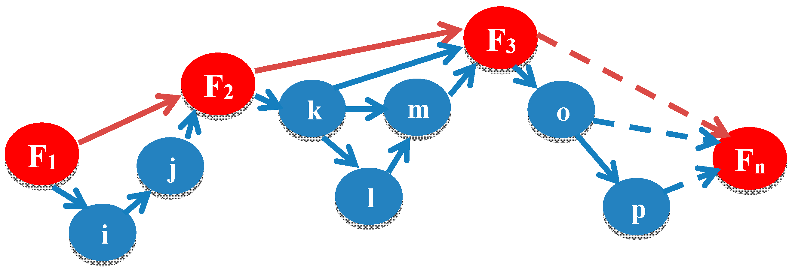
A general overview of the digraphs created by these profiles is shown in Figure 11, with the particularity that all paths must go through the funicular nodes (F_i).

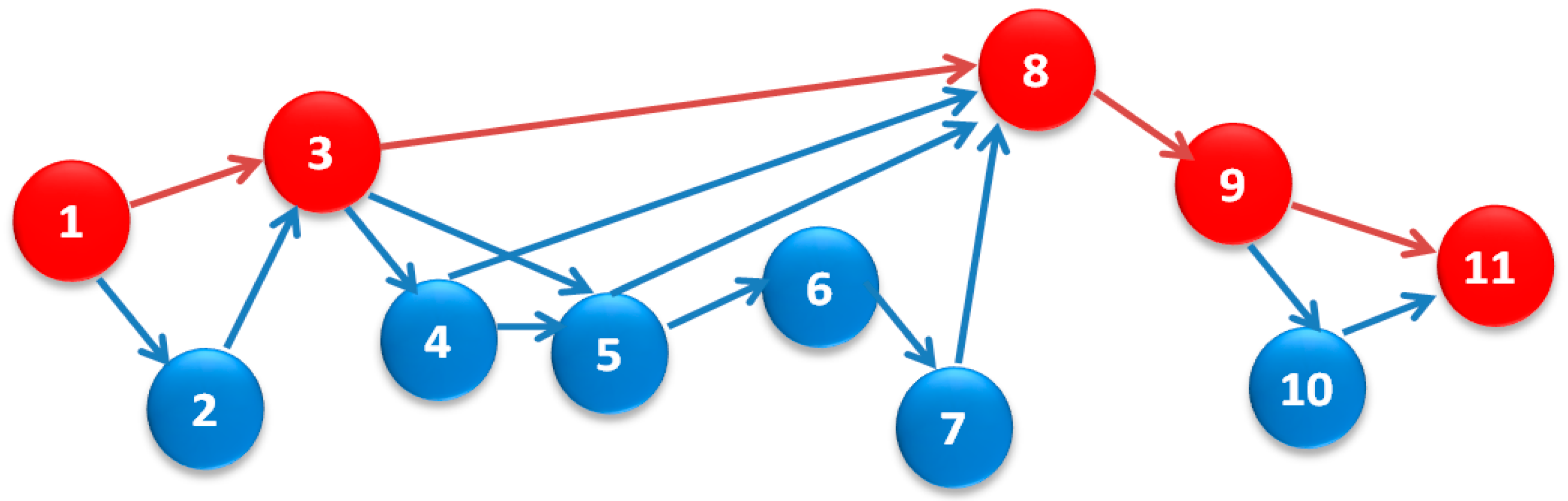
The graph obtained from the adjacency matrix of the final profile of the example of Figure 10, including ground reflection nodes, can be seen in Figure 12, where the funicular nodes are 1, 3, 8, 9 and 11:

As can be observed in Figure 12, up to eleven nodes in the worst case could be part of any path, wi, between the source and the receiver, considering diffraction and reflection nodes.

2.4. Pathfinding with the Breadth-First Search (BFS) Method

Once the adjacency matrix of LOS between selected nodes is built, the algorithm starts to identify all the possible paths between the source and the receiver. For this purpose, a breadth-first search (or traversal) method is programmed [16]. Starting on node v, the steps to be followed are:

• first, visit v;
• then, all its adjacent vertices are visited;
• next, those adjacent to the latter are visited, and so on.

The maximum number of possible paths between the source and the receiver can be easily determined in advance by [16]:

$$Paths={\displaystyle {\displaystyle \sum }_{i=1}^V}{A}^i\left[1\right]\left[V\right]$$

(6)

Therefore, the total feasible paths for the previous example, once properly filtered (Figure 12), would be 32.

The adjacency matrix, as well as the pathfinding, will be carried out again in each Fresnel frequency sub-band, so that the process of calculating the final sound pressure level will be significantly accelerated, since the number of nodes and paths will also appreciably decrease.

The importance of the process of selecting relevant nodes according to its influence in the final sound pressure field can be better understood if the same process is carried out without discarding any obstacle. In such a case, in the example of Figure 2, the total nodes (including reflections) would sum up 21 nodes, which would increase the number of possible paths of the equivalent graph up to 2291.

Moreover, it is also paramount to constrain the maximum number of hops or links when searching the possible paths from the source to the receiver, especially when the total amount of nodes of the final scenario is high. For this reason, the software code developed allows us to also manually or automatically tune this parameter.

2.5. Calculation of Total Sound Pressure Field at the Receiver

Following the previous task, the path matrix is now properly rearranged and sorted from the shortest path to the longest one, according to their number of nodes.

A loop then runs each frequency bin, from the minimum to the maximum, to provide the total sound pressure field for the complete set of paths for such a frequency. For each frequency, the algorithm also allows us to check the sound pressure field level at the receiver for each path. As the set of paths is sorted, it is expected that the subsequent sub-fields will be progressively decreasing, so that an adjustable threshold condition is defined in order to interrupt the addition of new fields if the current field is below the threshold. Such a threshold can be defined as the absolute value of the ratio between the level of signal received for the shortest path at such a frequency and the level of signal received for the current path (e.g., 1 × 10⁻⁴). Therefore, a threshold level of 0 would imply not discarding any path.

It should be noted that the computational time of the proposed algorithm is frequency-independent when the threshold is set to 0 and can always be limited or restrained, since the worst case can be foreseen in advance just by multiplying the consumed time at any frequency by the number of frequency bins considered in the simulation.

Regarding the above, the expression to obtain the complex field at the receiver, for each path i and each frequency is:

$${\varphi }_t{}_{pathi}=\frac{{\varphi }_0}{s_T}·e^{-jk{s}_T}·{\displaystyle {\displaystyle \prod }_{n=1}^{N-2}}\left(\begin{array}{c}{D}_n\\ R_n\end{array}\right)·\sqrt{\frac{s_T}{{{\displaystyle \prod }}_{i=1}^{N-1}\left(s_k\right)}}·\gamma$$

(7)

where:

${\varphi }_0$ is the sound pressure level transmitted by the source;

$s_T={\sum }_{i=1}^N{s}_i$, with $s_i$ being the slant distances of the links of the selected paths, between the geometrical centers of each node;

N is the number of nodes of each path;

$k$ is the wavenumber;

$D_n$ and $R_n$ are the diffraction or reflection coefficients, respectively, applied depending on the type of incidence to either the obstacles or the ground;

$\gamma$ is the obstacle coefficient factor. This expression comes from [10] and [11] but including, in this case, the $\gamma$ coefficient factor with two purposes: to adjust the phase, and as a weight factor ([3,6]), for each kind of obstacle considered in the present work.

The total sound pressure at the receiver for each frequency bin will be the summation of all the sound pressure signals for all the selected paths arriving to the receiver, as shown in Equation (1).

It should be noted that the $e^{+i\omega t}$ time-dependence term has been implicitly assumed and suppressed throughout the present study.

Next, the different coefficients considered in Equation (7) will be properly explained.

2.5.1. Obstacle Coefficient Factor γ

By means of the γ factor, the general expression in Equation (7) considers the specific modifications of the amplitude (spreading factors) to be applied depending on the type of obstacles, diffractions or reflections for the path under analysis. Otherwise, such an expression would only be applicable for knife edges and wedges. At the beginning of each path iteration, γ is reset to 1 and is progressively adjusted when considering either reflections on the ground or diffractions over obstacles between the two ends of the path:

• $\gamma \left(n\right)=\gamma \left(n-1\right)·{\gamma }_R$, ground reflection case, where n is the index of the current obstacle of the path, with

  $${\gamma }_R=\frac{A_R}{A_D}, A_R=\frac{s_i}{s_{i+1}+s_i},A_D=\sqrt{\frac{s_i}{s_{i+1}·\left(s_i+s_{i+1}\right)}}$$

  (8)
• $\gamma \left(n\right)=\gamma \left(n-1\right)·{\gamma }_b$, diffraction over wide barriers case, with [6]

  $${\gamma }_b=\{\begin{array}{c}1, if the edges of the obstacle\\ and the receiver are not connected\\ \\ 0.5, if the edges of the obstacle\\ and the receive are connected\end{array}$$

  (9)
• $\gamma \left(n\right)=\gamma \left(n-1\right)·{\gamma }_c$, diffraction over cylinders case, with

  $${\gamma }_c=\{\begin{array}{c}1,\hspace{1em}LOS between Tx and Rx, lit region\hfill \\ \\ \frac{A_{D1}}{A_{D2}}·\frac{e^{-ik\left(ta+s{s}_{i+1}-s_{i+1}\right)}}{e^{-ik\left(s_i-s{s}_i\right)}},\hspace{1em}shadow region\hfill \end{array}$$

  (10)

With

$$A_{D1}=\sqrt{\frac{s{s}_i}{s{s}_{i+1}·\left(s{s}_i+s{s}_{i+1}\right)}}$$

(11)

$$A_{D2}=\sqrt{\frac{s_i}{s_{i+1}·\left(s_i+s_{i+1}\right)}}$$

(12)

where:

• ss_i is the distance of the incident ray impinging on the cylinder;
• ss_i+1 is the distance of the diffracted ray from the cylinder to the next end;
• and ta is the arc length traveled by the creeping wave over the cylinder from the incidence point to the exit one.

2.5.2. Diffraction Coefficient for Knife Edges, Wedges and Wide Barriers

The computation of the diffraction coefficients for each type of obstacle are well known in the specific literature. For knife edges and wedges, the UTD expresses the acoustic diffraction coefficient for an infinitely long knife edge or wedge as [11]:

$$\begin{array}{c}D\left(v,k,L,s1,s2,{\theta }_2,{\theta }_1\right)\hfill \\ =\frac{-e^{-i\frac{\pi }{4}}}{2v\sqrt{2\pi k}}·\left[\begin{array}{c}ta{n}^{-1}\left(\frac{\pi +\left({\theta }_2-{\theta }_1\right)}{2v}\right)·F\left(kL{a}^{+}\left({\theta }_2-{\theta }_1,v\right)\right)\\ +ta{n}^{-1}\left(\frac{\pi -\left({\theta }_2-{\theta }_1\right)}{2v}\right)·F\left(kL{a}^{-}\left({\theta }_2-{\theta }_1,v\right)\right)\\ +R_n·ta{n}^{-1}\left(\frac{\pi +\left({\theta }_2+{\theta }_1\right)}{2v}\right)·F\left(kL{a}^{+}\left({\theta }_2+{\theta }_1,v\right)\right)\\ +R_0·ta{n}^{-1}\left(\frac{\pi -\left({\theta }_2+{\theta }_1\right)}{2v}\right)·F\left(kL{a}^{-}\left({\theta }_2+{\theta }_1,v\right)\right)\end{array}\right]\hfill \end{array}$$

(13)

where $R_0$ and $R_n$ are the reflecting coefficients of the adjacent and opposite obstacle faces seen by the incident wave, respectively (a more detailed explanation of the other parameters can be found in [11]).

In the previous expression, the following approximation can be carried out when the cotangent terms in Equation (13) are singular at a reflection or a shadow boundary [11]:

$$ta{n}^{-1}\left(\frac{\pi \pm \beta }{2v}\right)F\left(kL{a}^{\pm }\left(\beta ,v\right)\right)\approx v{e}^{-i\frac{\pi }{4}}·\left(\sqrt{2\pi kL}·sign\left(\epsilon \right)-2kL\epsilon e^{-i\frac{\pi }{4}}\right)$$

(14)

where $\epsilon$ fulfills the expression:

$$\beta =2\pi N^{\pm }\mp \left(\pi -\epsilon \right)$$

(15)

The same solution can be used, without losing any accuracy, for the case of diffraction over wide barriers, just by considering a barrier as two joined (interconnected) wedges of interior angle π/2 rad and using the proper correction factor.

2.5.3. Diffraction Coefficient for Cylinders (Rounded Obstacles)

The UTD comprises two scattering mechanisms for cylindrical structures, which are either the reflection or the diffraction components of the field [17,18,19].

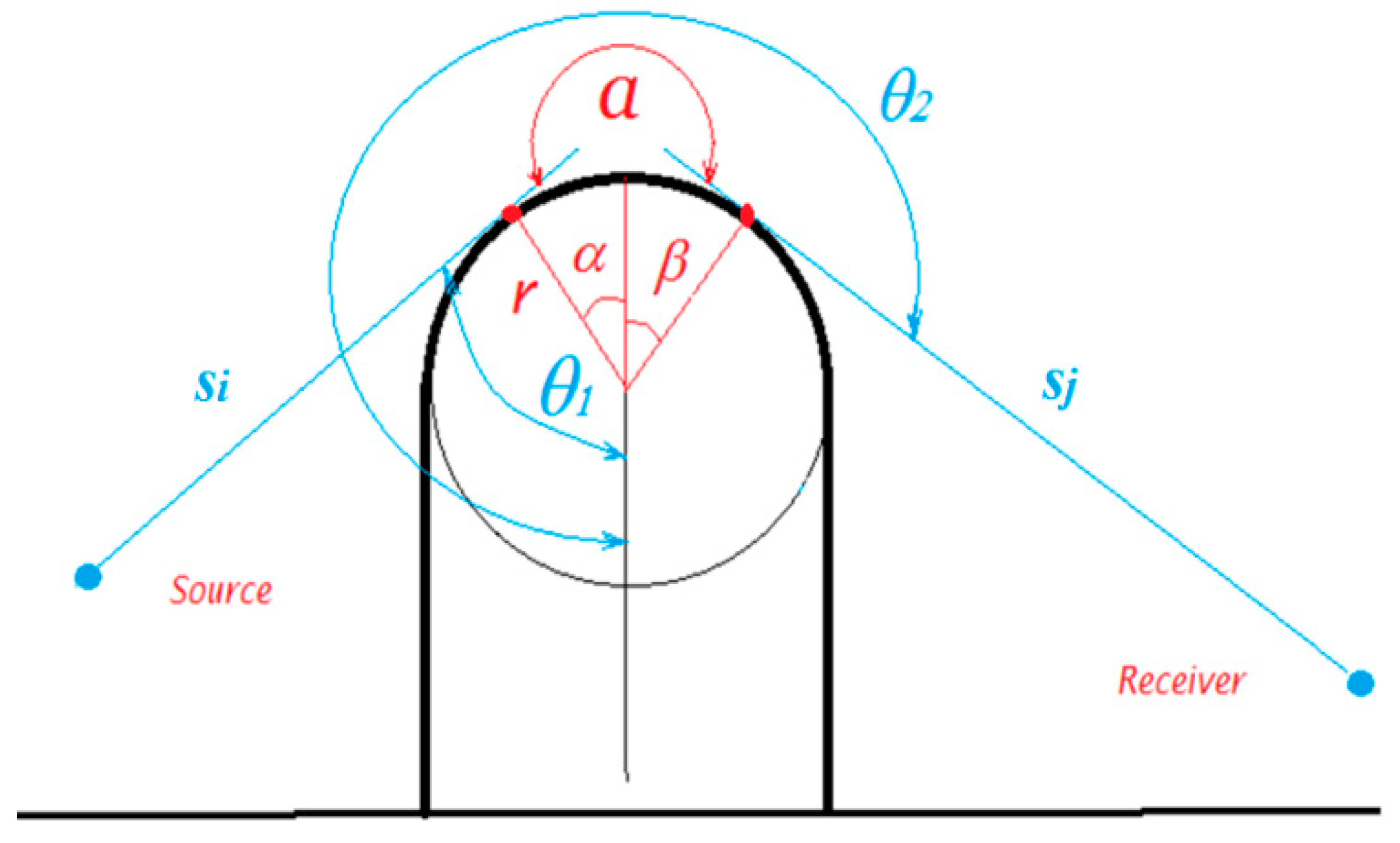
For the so-called shadow region (no LOS between the source and the receiver), the following diffraction coefficient can be considered:

$$T_{s,h}\left(a\right)=m_p\sqrt{\frac{2}{k}}{e}^{-i\frac{\pi }{4}}{e}^{-ikt\left(a\right)}\left\{\frac{-F\left[x\left(a\right)\right]}{2\epsilon \left(a\right)\sqrt{\pi }}+\left[q^{\ast }\left(\epsilon \left(a\right)\right)\right]\right\}$$

(16)

With

$$a=\pi +\alpha +\beta , \alpha ,\beta \ge 0$$

(17)

$$X\left(a\right)=\frac{kL{\left(a-\pi \right)}^2}{2}$$

(18)

$$L=\frac{s_i{s}_j}{s_i+s_j}$$

(19)

$$\epsilon \left(a\right)=m_p\left(a-\pi \right)$$

(20)

$$={\left(\frac{k·r_{obs}}{2}\right)}^{\frac{1}{3}}$$

(21)

where α and β are the angles of the arc run by the creeping wave over the cylinder, k is the wavenumber, $r_{obs}$ is the radii of the cylinder and s_i and s_j are the slant ranges, as shown in Figure 13.

The first addend of Equation (16) describes the Fresnel diffraction process. F[x] is the so-called transition function, which is defined in terms of a Fresnel integral [11]:

$$F\left[x\right]=2i\sqrt{x}{e}^{ix}{{\displaystyle \int }}_{\sqrt{x}}^{\infty }{e}^{-i{u}^2}du$$

(22)

In the second addend of Equation (16), the term q*(ε(a)) is the so-called Fock scattering function, and addresses the generation of creeping waves along the surface of a smooth body, such as spheres or cylinders [17]:

$$q^{\ast }\left(x\right)=\frac{1}{2\sqrt{\pi }x}+\frac{1}{\sqrt{\pi }}{{\displaystyle \int }}_{-\infty }^{\infty }\frac{V^{\prime \left(t\right)}}{w_2^{\prime }\left(t\right)}{e}^{-ixt}dt$$

(23)

(the prime represents differentiation with respect to argument), where V(t) and w₂(t) are defined as:

$$V\left(t\right)=\sqrt{\pi }{A}_i\left(t\right)$$

(24)

$$w_2=2\sqrt{\pi }{e}^{-i\frac{\pi }{6}}{A}_i\left(t{e}^{-i\frac{2\pi }{3}}\right)$$

(25)

with A_i(t) as a Miller-type Airy function:

$$A_i\left(t\right)=\frac{1}{\pi }{{\displaystyle \int }}_0^{\infty }cos\left(\frac{1}{3}zs+tz\right)dz$$

(26)

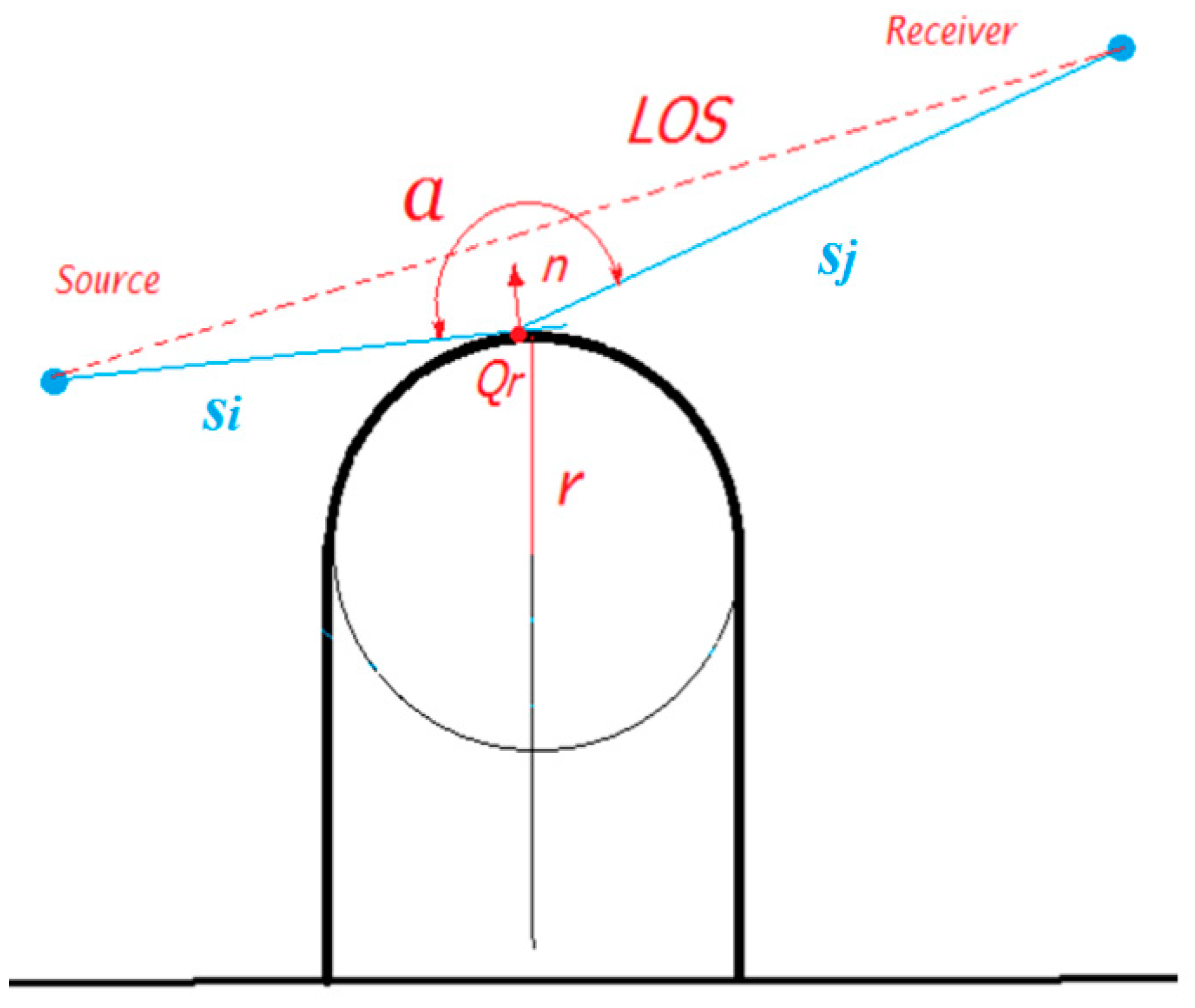
For the so-called lit region (LOS between the source and the receiver), the following diffraction coefficient is applicable instead:

$$R_{s,h}\left(a\right)=\sqrt{\frac{r}{m^{\prime }}}{e}^{-i\frac{{\epsilon }^3\left(a\right)}{12}}{e}^{-i\frac{\pi }{4}}\left\{\frac{-F\left[x\left(a\right)\right]}{2\epsilon \left(a\right)\sqrt{\pi }}+\left[q^{\ast }\left(\epsilon \left(a\right)\right)\right]\right\}$$

(27)

where a is again the angle between the incident and the diffracted ray, as given in Figure 14, and:

$$\epsilon \left(a\right)=-2m_p\left(\cos \left(\frac{a}{2}\right)\right)$$

(28)

$$X_a=2kL{\left(\cos \left(\frac{a}{2}\right)\right)}^2$$

(29)

with L as in Equation (19).

For the case of grazing incidence in rounded surfaces, with an almost equal to π, it is required to proceed in a similar way as in the case of knife edges or wedges, but adding another term that accounts for the curvature of the obstruction, as also happens in radio wave propagation [18]:

$$D_{cylinder}=D_{knifeedge}-m_p\sqrt{\frac{2}{k}}{e}^{-i\frac{\pi }{4}}{q}^{\ast }\left(\epsilon \left(a\right)\right)$$

(30)

2.5.4. Ground Reflection Coefficient

Ground reflection is considered as any other node of the scenario. Although the reflection coefficient Rn can be adjusted in the proposed method and it depends on the acoustic impedance of the material and the angle of incidence, it is usually fixed to 1 (perfect reflection) throughout the present work for comparison purposes with other existing models.

Once the total sound pressure field is calculated at the receiver, or final node, for a specific frequency, the insertion losses (IL) at such a frequency can be estimated by [6]:

$$IL\left(dB\right)=20·{\log }_{10}\left(\left|\frac{{\varphi }_t{}_{Rx}}{{\varphi }_{fs}}\right|\right)$$

(31)

where ${\varphi }_t{}_{Rx}$ is the sound pressure field at the receiver considering obstacles and ${\varphi }_{fs}$ is the sound pressure field at the receiver in free space (without considering obstacles).

It should be noted that the parameter ${\varphi }_{fs}$ must also account for the single reflection on the ground in the absence of obstacles.

3. Results and Discussion

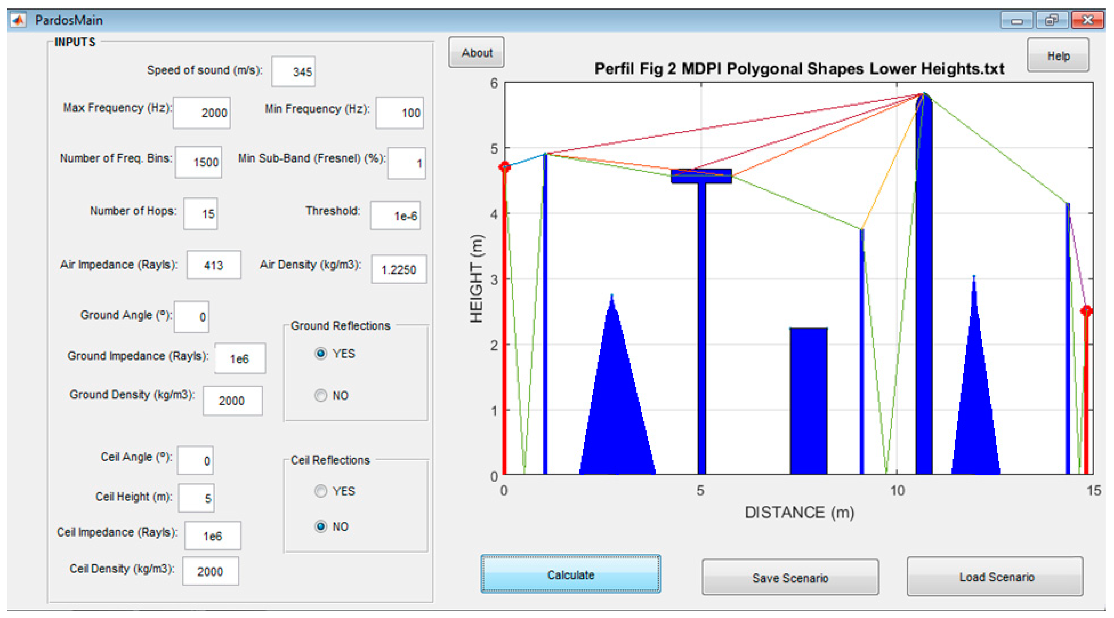
Firstly, the IL of the scenario of the example of Figure 2 was obtained following all the steps mentioned in Section 2. For that purpose, a software tool was developed by the authors using the interactive programming environment and pre-built computational libraries of MATLAB [20]. The graphical user interface of the software tool can be observed in Figure 15.

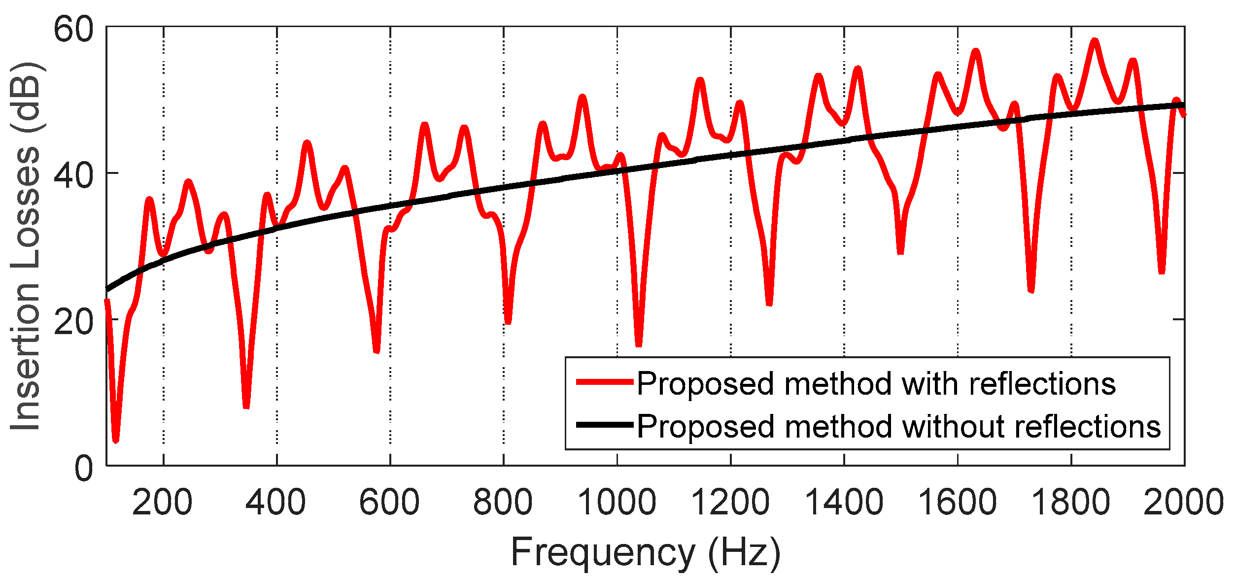
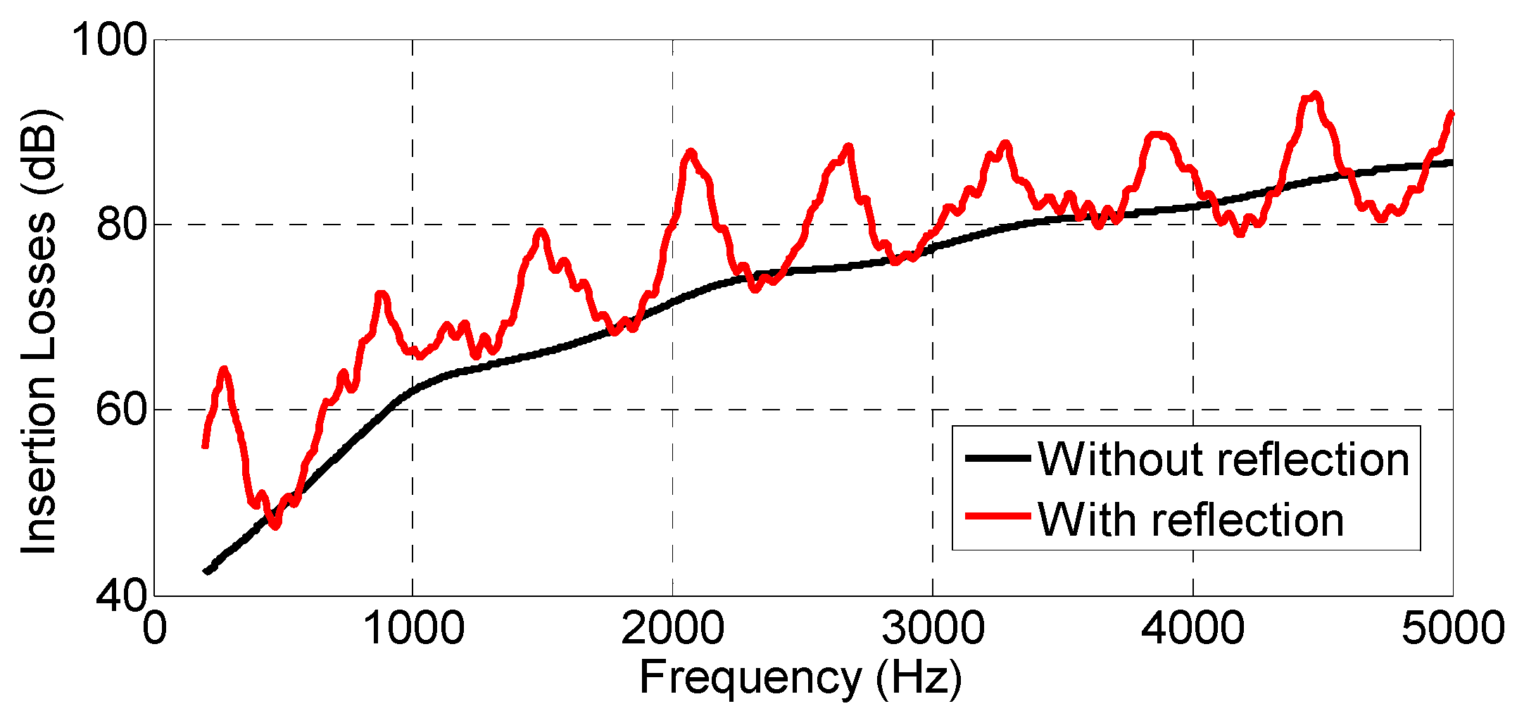
The IL at the receiver, as a function of frequency, can be observed in Figure 16, with and without reflections on the ground. It should be noted that the calculations for such figure only took 15.1 s with reflections on the ground and 1.62 s for that without reflections. The computer selected to run all the simulations throughout the present work was an Intel(R) Xeon(R) CPU E3-1231 v3 @ 3.40 GHz with 16 GB of RAM.

It should be noted that, in spite of ignoring the obstacle node 7 of Figure 8 from 123.6 Hz and obstacle nodes 3 and 4 from 1777.6 Hz onwards (due to the fact that the radius of the Fresnel zone decreases with frequency), the IL curve in the results of Figure 16 continued its increasing behavior up to 2000 Hz due to the fact that the diffraction coefficient also decreases with frequency.

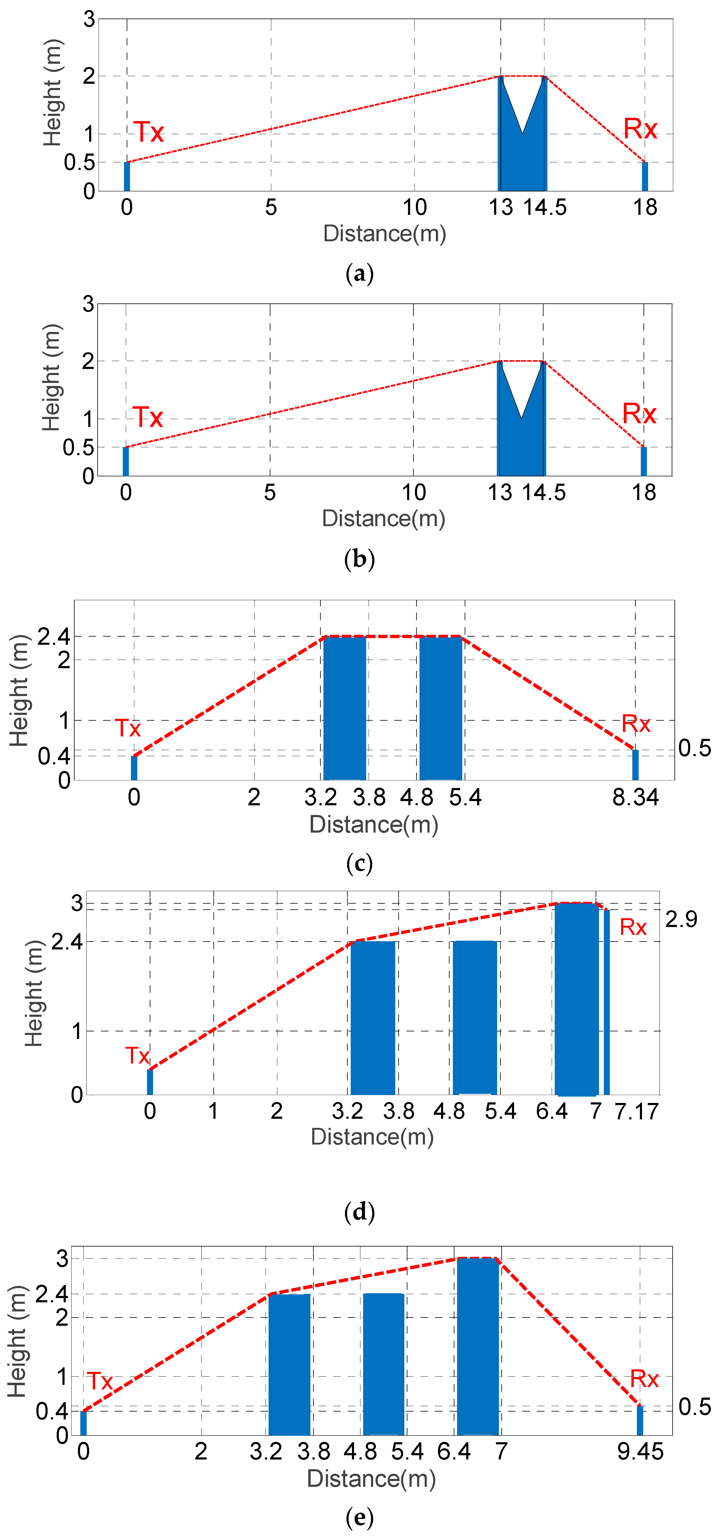
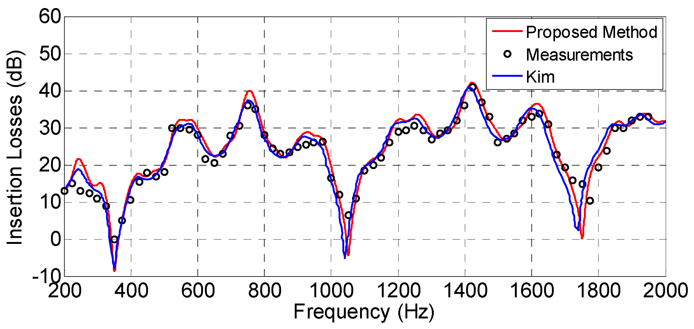
The proposed method was properly compared with other validated formulations published by other authors, considering different scenarios (including different types of obstacles), in order to verify its accuracy. In Figure 17, the different scenarios considered for the validation of the proposed model are shown.

Firstly, in Figure 18 and Figure 19, the IL as a function of frequency are compared with the IL provided by Kim et al. [5] (scenarios and parameters taken from Figure 4 and Figure 9 of [5], respectively) for a double knife edge case (Figure 17a) and a double wedge case (Figure 17b). In Figure 18, the measurement data taken from [21] are also depicted for comparison.

As can be observed, good agreement is obtained between the proposed method and the formulation presented in [5] in both cases, taking our solution simulation times of only 1.27 and 0.94 s in Figure 18 and Figure 19, respectively, for the obtaining of the IL in the whole frequency range (with 1500 frequency bins). Moreover, the agreement of the results obtained with the proposed method with the measurements in Figure 18 seems to be better in some frequencies—especially in the valleys of the curve—than those achieved by Kim et al.

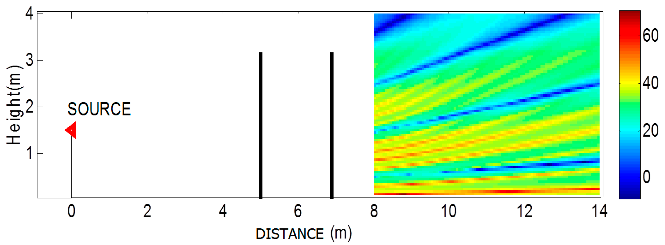
The proposed method can also provide the IL map as a function of the receiver location at any frequency. In Figure 20, an example of such an application is depicted for the same scenario as that of Figure 17a for 1 kHz (double knife edge barrier).

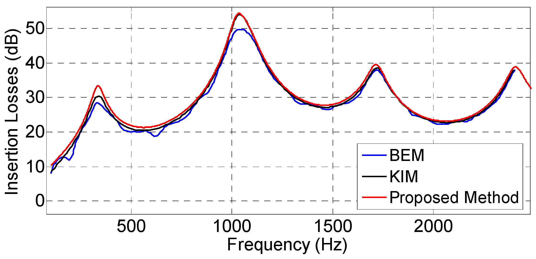
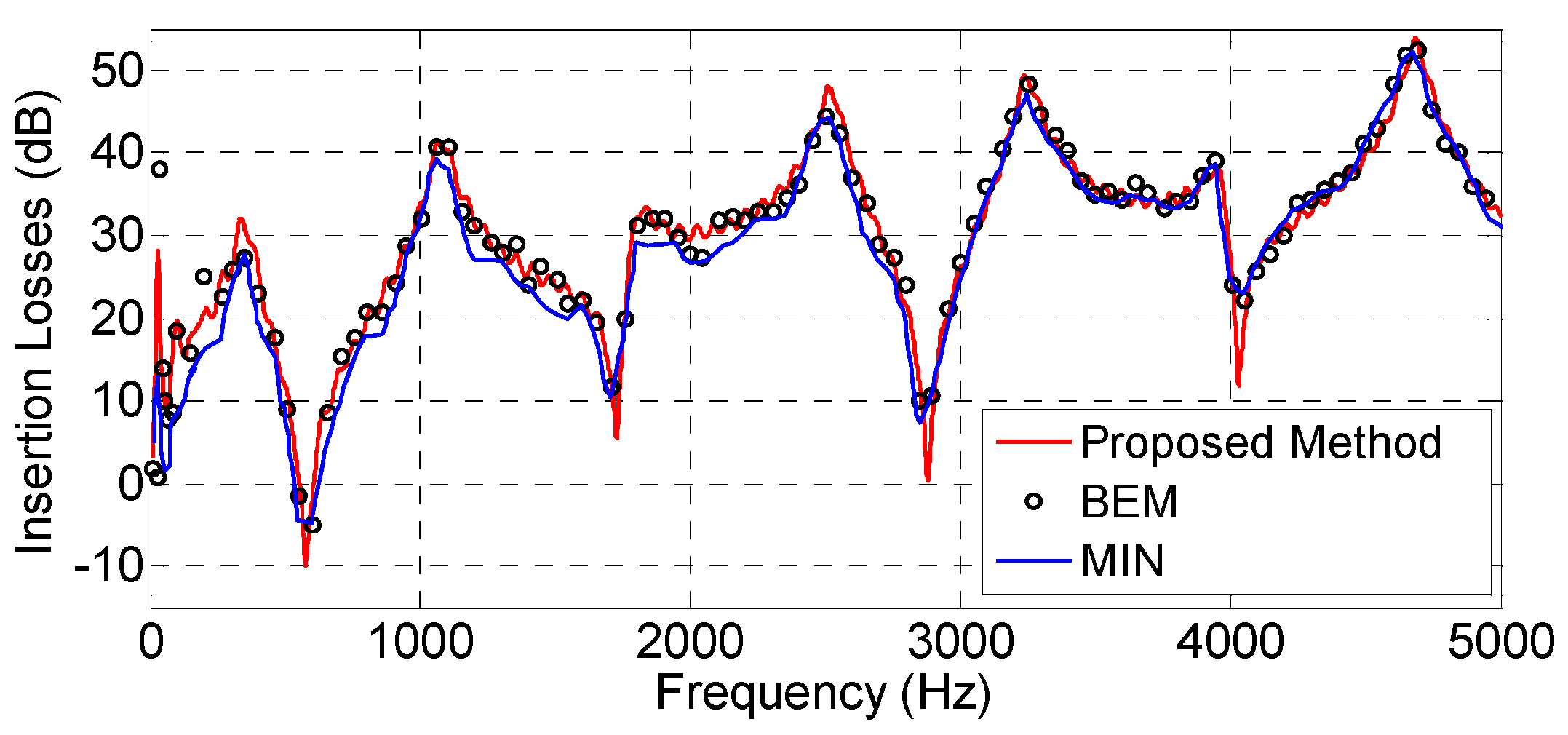
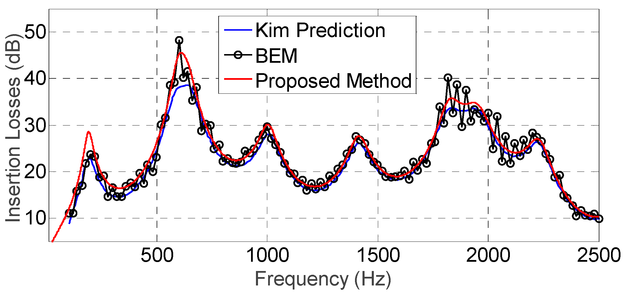
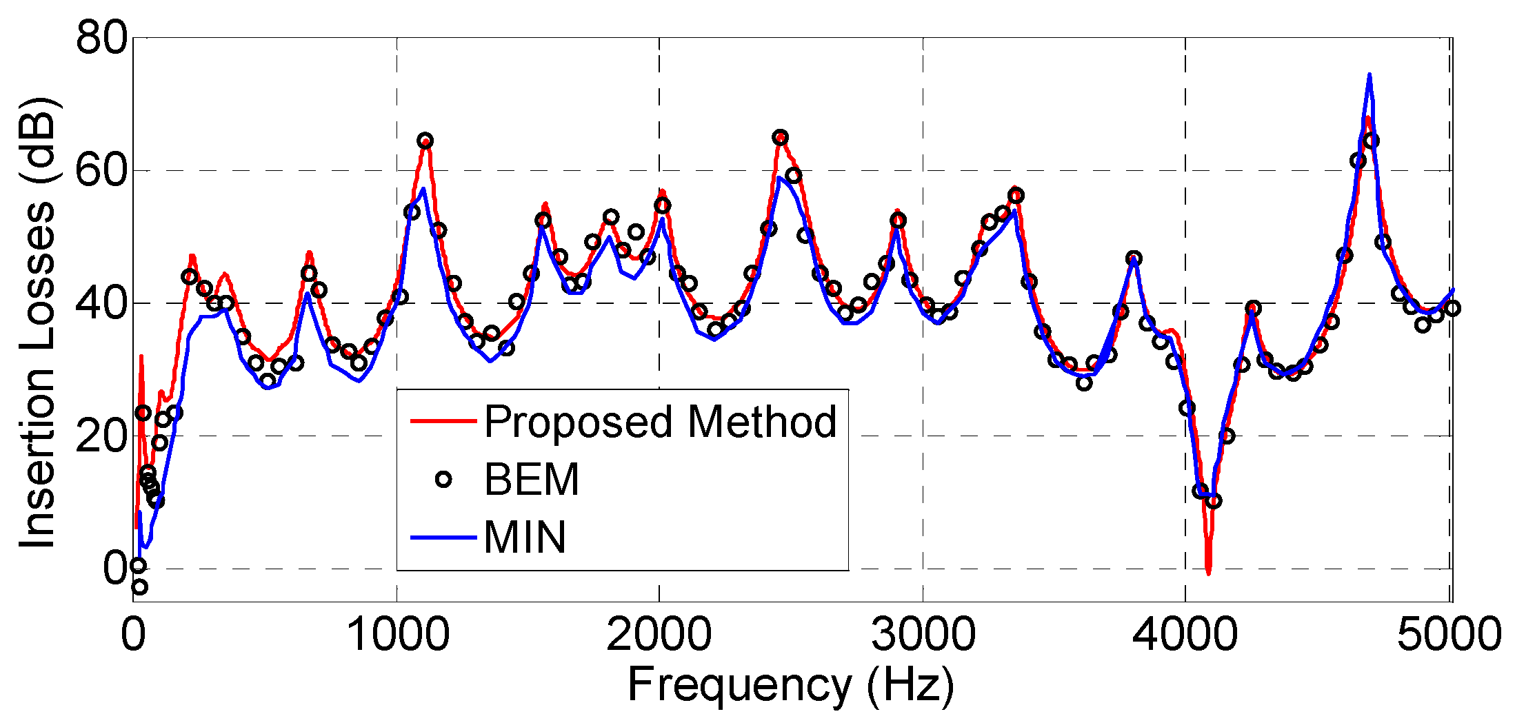
The IL for a scenario with a different distribution of wide barriers and several locations of transmitters and receivers were also simulated by our method and properly compared with other formulations. For that purpose, the IL for the scenarios of Figure 17c–e (cases analyzed by Min and Qiu in Figure 7, Figure 8 and Figure 9 of [6]) are displayed in Figure 21 and Figure 22, respectively. The numerical results obtained by the BEM are also shown in the plots.

As can be observed, good agreement is again obtained in the three wide barrier cases between the proposed method and both the BEM and Min and Qiu methods. In fact, the agreement between the BEM and our method seems to be better than the results of Min and Qiu. The simulation times for Figure 21, Figure 22 and Figure 23 (with 2500 frequency bins) were 3.91, 11.98 and 13.89 s, respectively. It should be noted that, in the results of Figure 22 and Figure 23, the second wide barrier was discarded at 3066.7 Hz due to the decrease of the radius of the Fresnel zone with frequency, as previously mentioned, with the consequent reduction in terms of computational time.

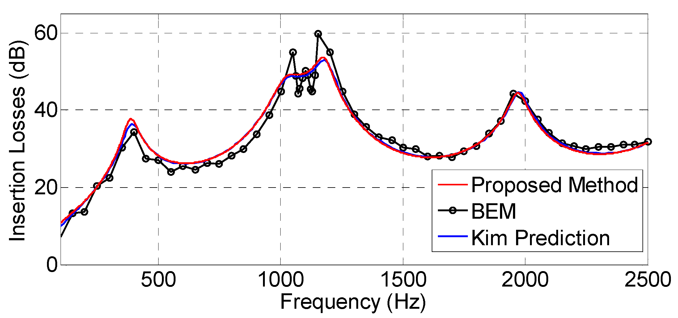
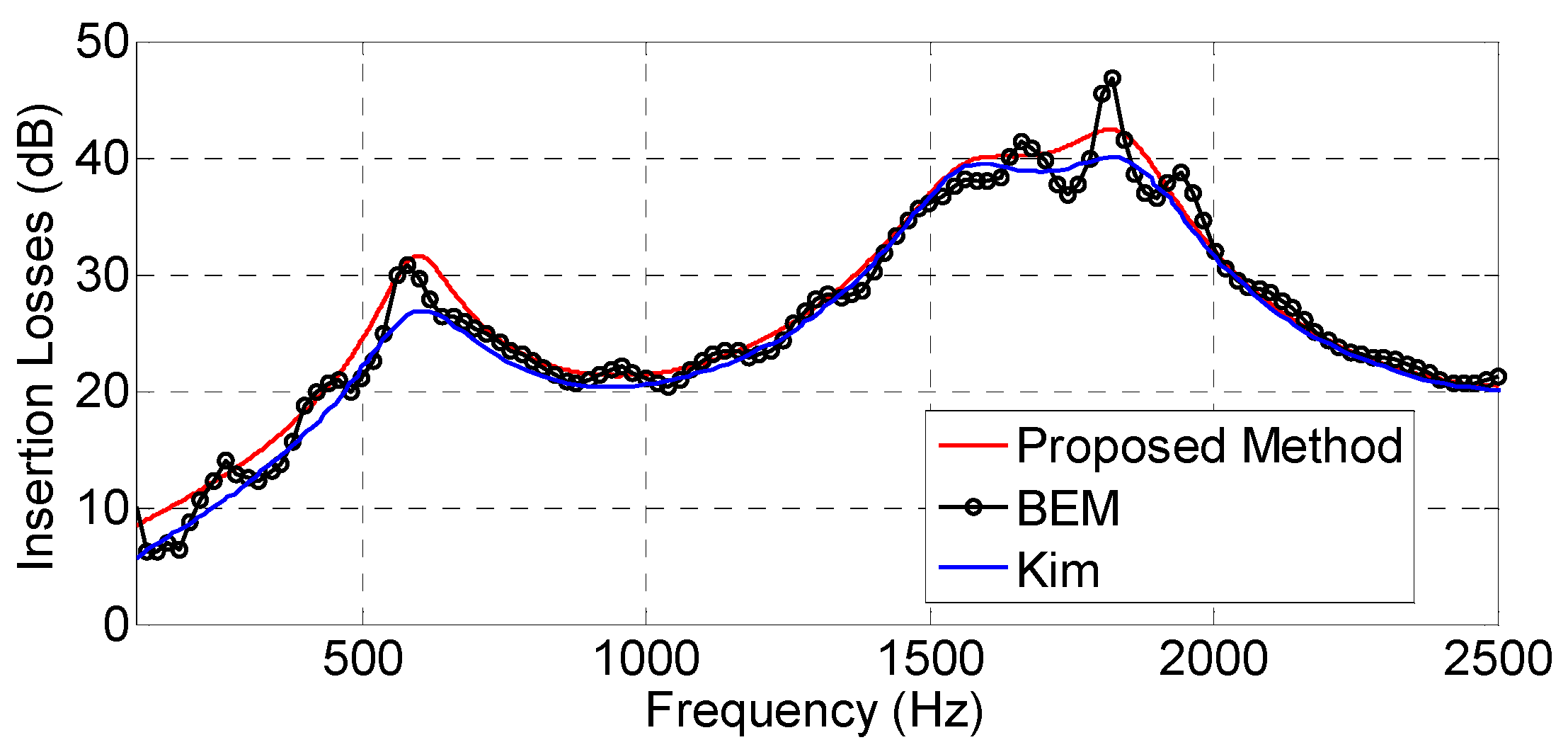
Following the comparison of the results obtained with knife edges, wedges and wide barriers, additional simulations of the expected IL for doubly inclined, Y- and T-shaped barriers were undertaken. Figure 24, Figure 25 and Figure 26 present the simulations for the scenarios depicted in Figure 17f–h (from Figure 13, Figure 15 and Figure 17 of [5]), respectively. The numerical results obtained by the BEM are also shown in the plots.

Once more, the comparison between the proposed method and both the BEM and Kim et al. formulation shows good agreement for the cases of doubly inclined, Y- and T-shaped barriers. In fact, again, the agreement between the BEM and our method seems to be better than with the Kim results. The required simulation times were, on this occasion, just 1.2, 1.4 and 1.0 s, respectively (with 1500 frequency bins).

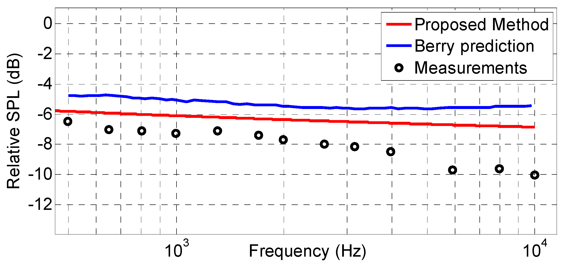
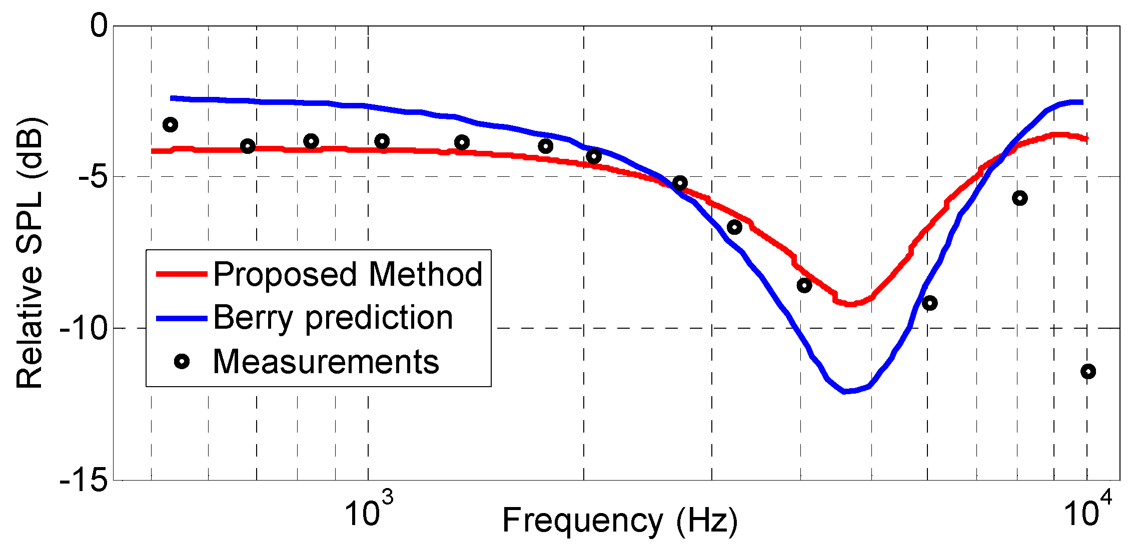
The next goal was to validate the algorithm for cylindrical obstacles. Unfortunately, the number of publications found by the authors in which diffraction measurements on rounded obstacles are presented is scarce. Nevertheless, the work of Berry and Daigle [22] should be highlighted, who published measurements of the relative sound pressure field for one rounded obstacle with a radius of 5 m and a receiver at different heights above a rigid surface, in the shadow boundary. The IL obtained with the proposed method and Berry and Daigle’s predictions for the two scenarios indicated in Figure 17i,j (from Figure 6b,c of [22]), where a cylindrical barrier is considered, are shown in Figure 27 and Figure 28. Some measurements performed by Berry and Daigle are also shown in the plots. It should be noted that the scenario of Figure 6a in [22] was not simulated as it considers the receiver on the surface of the own cylinder with a relative height of 0 m, where the present model would not be fully applicable.

As can be observed, the proposed method shows better agreement with the measurements than the predictions of Berry and Daigle. The proposed method took 0.75 and 0.76 s to complete the plots of Figure 27 and Figure 28, respectively (without considering reflections and 5000 frequency bins).

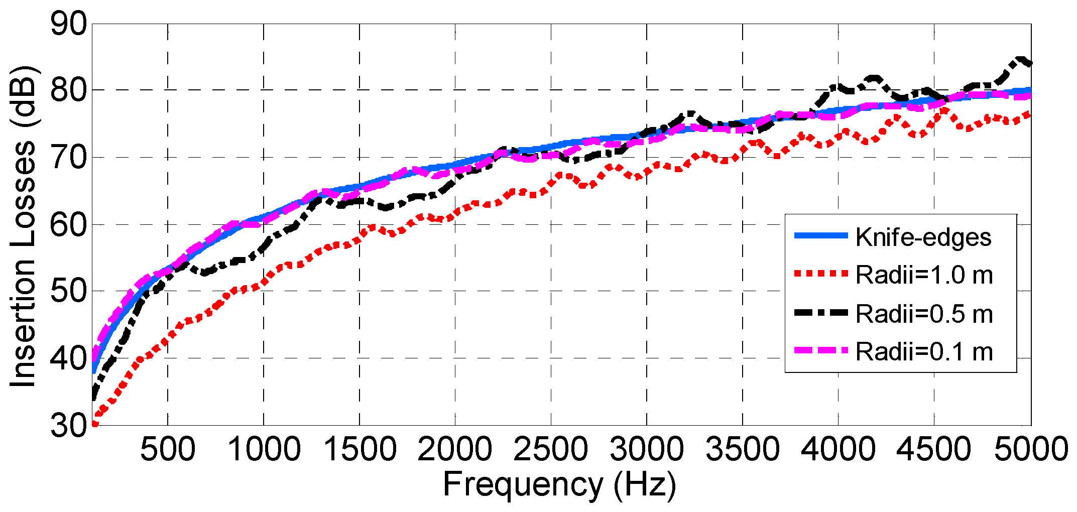
In order to also check the behavior of the algorithm for an array of rounded obstacles, a scenario filled with ten cylinders randomly allocated with different heights and the same radius was defined (Figure 29). Then, the IL results for cylindrical diffraction, without considering reflections on the ground, were compared with the asymptotic IL when the radius is decreased to almost 0 (knife edge case). It should be expected that the IL when considering cylinders would converge to the scenario where the obstacles are replaced by knife edges at the same locations and with the same heights. The results can be observed in Figure 30 for cylinders with radii of 1.0, 0.5 and 0.1 m.

As expected, the curves for the knife edges case and cylinders with a radius of 0.1 m practically coincide.

Analysis of Computational Efficiency of the Proposed Method

In order to analyze the computational efficiency of the proposed method, we will consider again the scenario of Figure 17e with three barriers, whose IL results are already shown in Figure 23. The full elapsed time to plot the whole IL results with our method (assuming 2500 frequency bins) was only 13.89 s, taking advantage of the funicular profiles, an optimum choice of nodes as a function of frequency by Fresnel ellipsoids, graph theory for the fast search and reordering of paths by number of hops and a threshold value to account for any path. In contrast, the time employed for the Min and Qiu method, for only one frequency and the same computer, was 2.6 min, which points to a much greater simulation time. The BEM results, which are frequency-dependent, such as OpenBEM [23], required more than half an hour per a single frequency bin and the same scenario of Figure 17e, which again is a much longer time compared to the method proposed in this work.

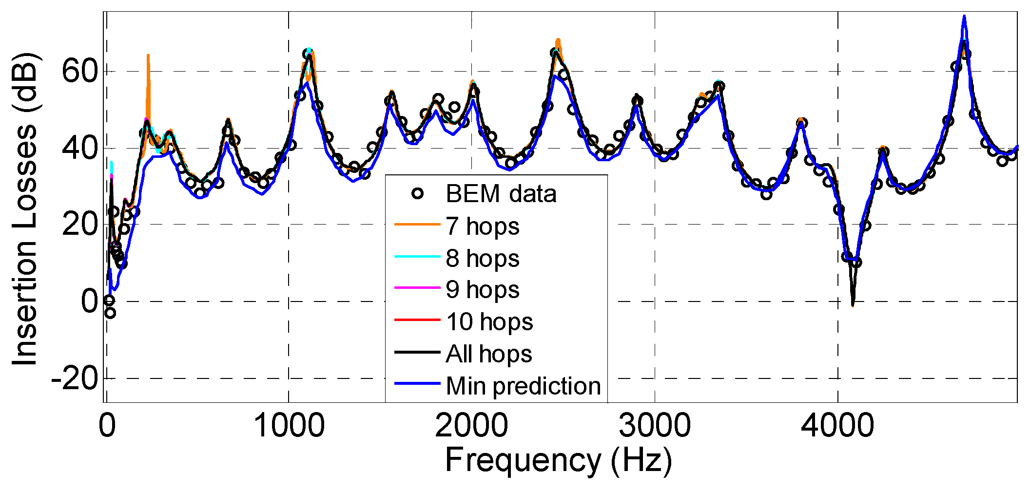
Moreover, in order to check the impact on accuracy of the IL estimated with our method when the maximum number of hops in the path is progressively reduced, Figure 31 is shown, where again the scenario of Figure 17e is considered. On this basis, the maximum number of hops in the scenario is progressively constrained (down to only seven hops) and a threshold criterion to add new paths is also kept (10⁻⁵). It should be noted that three wide barriers imply a maximum number of 12 nodes and 11 hops, including reflections.

As can be observed, even when the maximum number of hops is decreased down to seven or eight hops, the accuracy of the results obtained with the proposed method remains reasonable whilst simultaneously reducing the computational effort down to only 10 s (when limiting the maximum number of hops to eight).

Finally, in order to assess the potential and the efficiency in terms of computational time of the proposed method to estimate the IL at the receiver as a function of frequency, a completely heterogeneous and more complex scenario is finally considered in Figure 32, in which different types of obstacle modeling, heights and spacing are taken into account. When running the method, one obstacle is initially discarded at 200 Hz by the application of the Fresnel criterion at the distance of 15.2 m and 20 nodes. The transmitter, obstacles, reflections and receiver are then considered.

The IL as a function of frequency, with and without reflections on the ground, is shown in Figure 33.

The parameters of the simulations of Figure 33 and the obtained results are summarized in

Table 1. Parameters for Scenario of Figure 32.

Parameter	Result
Subbands [Hz]—by Fresnel ellipsoid analysis	[200–565.4], [565.4–646.9], [646.9–684.3], [684.3–1293.8], [1293.8–5000]
Final selection of nodes	20 (max. at lowest band) down to 12 (at highest band)
Hops selected	19 (max at lowest band) down to 11 (at highest band)
Paths selected	1800 (max. at lowest band) down to 20 paths (at highest band)
Frequency band [Hz]	200–5000
Frequency bins	1500
Minimum relative threshold level	10-5
Elapsed time without reflections [s]	1.81
Elapsed time with reflections [s]	19.02

.

One of the key strategies implemented within the present method relies on the gradual reduction of the relevant nodes in each frequency band. It should be noted how, even with the complexity of the scenario analyzed, the elapsed time of computation considering reflections on the ground was ~19 s, which points to the good computational efficiency of the proposed method.

Table 2. Summary of the simulation time for each scenario.

Scenario	Elapsed Time (s)
Figure 2	15.1
Figure 17a	1.27
Figure 17b	0.94
Figure 17c	3.91
Figure 17d	11.98
Figure 17e	13.89
Figure 17f	1.2
Figure 17g	1.4
Figure 17h	1.0
Figure 17i	0.75
Figure 17j	0.76
Figure 32	19.02

summarizes the analysis performed for up to 12 simulated scenarios. As can be observed, in all cases, the total computation time was well below 30 s (for 1500 frequency bins or higher), therefore dramatically improving the computation times required by BEM, which typically take more than 1 min just for one frequency bin (depending on the frequency under analysis and the obstacle shape).

4. Conclusions

In this work, an innovative, fast, UTD-based method for the analysis of multiple diffraction of acoustic waves when considering a series of obstacles with arbitrary modeling (knife edges, wedges, wide barriers, cylinders, doubly inclined and T-/Y-shaped barriers), height and spacing has been presented. The method, which makes use of funicular polygons, Fresnel ellipsoids and graph theory, and controls both the maximum number of hops and the minimum threshold criterium, has been properly compared and validated with other existing formulations as well as measurements showing good agreement while at the same time offering much better computational efficiency. On this basis, a great number of obstacles (including neighboring ones of equal height) forming a very complex scenario can be analyzed in an acceptable time.

The potential of the proposed method in terms of computational time is due to the fact that it allows for an optimum selection of the prominent obstacles, processes them as nodes of a graph, identifies and rearranges the paths reaching the receiver, constraints the maximum number of hops and permits defining a threshold criterion to discern the relevant paths.

Future work will be focused on the performance of an extensive measurement campaign undertaken in real scenarios to explore the limits in which the proposed method remains valid. Moreover, the authors’ future interest will be paid on reviewing, extending and validating the present method for more complex scenarios involving 3D profiles, as well as other polygonal structures while further achieving improved computational efficiency. Finally, the authors’ attention will also include the characterization of the acoustic impedance of the barriers for extending the model to a wider range of scenarios and applications.