Handling Covariates in Markovian Models with a Mixture Transition Distribution Based Approach

Abstract

This paper presents and discusses the use of a Mixture Transition Distribution-like model (MTD) to account for covariates in Markovian models. The MTD was introduced in 1985 by Raftery as an approximation of higher order Markov chains. In the MTD, each lag is estimated separately using an additive model, which introduces a kind of symmetrical relationship between the past and the present. Here, using an MTD-based approach, we consider each covariate separately, and we combine the effects of the lags and of the covariates by means of a mixture model. This approach has three main advantages. First, no modification of the estimation procedure is needed. Second, it is parsimonious in terms of freely estimated parameters. Third, the weight parameters of the mixture can be used as an indication of the relevance of the covariate in explaining the time dependence between states. An illustrative example taken from life course studies using a 3-state hidden Markov model and a covariate with three levels shows how to interpret the results of such models.

1. Introduction

Markovian models are stochastic models dedicated to the analysis of the transitions between successive states in sequences. More specifically, a Markovian model aims to describe how the current distribution of the possible values of a characteristic of interest depends on its previously observed values. Markovian models in their traditional formulation are used to study the behavior of a single variable. However, using longitudinal data, it is natural to describe the dynamics of the outcome variable according to the effect of external factors—or in other words, to study how the time dependence among observations is moderated by other variables.

This paper discusses a Mixture Transition Distribution (MTD)-based approach to handle covariates in Markovian models. The MTD has been introduced in the literature as an approximation of high-order Markov processes [1]. In the MTD, the effect of each additional lag upon the present is considered as only one additional parameter in the model [2], in this sense, an MTD introduces a kind of symmetrical relationship between the past and the present. Similarly, this paper presents an approach to account for covariates in Markovian modeling, considering each covariate as additional exploratory terms. In a nutshell, we consider the effects of the lag(s) and of each covariate separately and we combine them by means of a mixture model.

Several models to account for categorical covariates in Markovian modeling have been presented in the literature, such as considering all possible interactions between the state of the model and levels of the covariates or a parametrization of the transition probabilities using a multinomial model for example. The advantages of the MTD-based approach discussed here are that it does not require any modification of the estimation procedure with respect to a model without covariates and we do not need to estimate a potentially very large transition matrix made by the interaction between states and levels of the covariates.

The article is organized as follows. Section 2 sets the general framework of Markov chain, the Mixture Transition Distribution model, and the hidden Markov model. Section 3 discusses how to consider covariates in Markovian models using an MTD-based approach. Then, an empirical example is shown to illustrate the proposed approach in the framework of a hidden Markov model (Section 4). Finally, Section 5 recaps the advantages of using such an approach to handle categorical covariates in Markovian modeling.

2. Markovian Models

2.1. The Markov Chain

A discrete-time Markov chain is a stochastic process that models the serial dependence between values in adjacent periods [3]. It describes the movement through a finite number of predefined categorical states that are assumed to be mutually exclusive.

Let $X_t$ be a random variable taking values in a finite set with $t=0,1,2,\dots ,T$. A Markovian process models the transition probabilities, that is the probability distribution of the state $x_t$ to be observed at time t given the modalities observed in the previous period(s).

In its conventional formulation, a Markov chain is a memoryless process. The next modality of the variable depends only on the current state that is assumed to summarize the whole time series. This is known as the “Markov property” and it defines a first-order Markov chain.

The probability of switching from a given state to another is often assumed to remain unchanged over time. This defines a time-homogeneous Markovian process with transition probabilities reading for a first-order Markov chain as $Pr(X_t=j\mid X_{t-1}=i)=a_{ij}$ whatever $t=1,\dots ,T$ and $i;j=1,\dots ,m$, where m is the number of states. The transition probabilities are generally represented in a square matrix of order m known as the transition matrix. Each row of this matrix represents a probability distribution and therefore, sums to one. The number of free parameters to estimate in a first-order homogeneous Markov chain is then equal to $m(m-1)$.

2.2. The Mixture Transition Distribution Model

The assumption of having a process of order one is often too simplistic and can be overcome with higher order Markov chains where the next state depends on the f previous states. However, the problem is that the number of independent parameters increases exponentially with the order of the chain. The total number of transition probabilities to estimate in a homogeneous Markov chain of order f is $m^f(m-1)$, where m is the number of states. Therefore, very large datasets may be required to accurately estimate all transition probabilities. We might even encounter identification problems when the amount of data is too small.

A parsimonious way to work with high-order Markov chains is the Mixture Transition Distribution model (MTD). In the MTD, introduced by Raftery in 1985 [1], the idea is to consider separately the effect of each lag on the current state instead of considering the effect of the combination of the previous f states. The model is written as follows:

$$P(X_t=x_t|X_{t-1}=x_{t-1},\cdots ,X_{t-f}=x_{t-f})\cong \sum _{g=1}^f{\lambda }_g{a}_{x_{t-g}{x}_t},$$

(1)

where ${\lambda }_g$ is a weight parameter associated to lag g and $a_{x_{t-g}{x}_t}$ is the transition probability from the state at time $t-g$ to the current one $x_t$. The same transition probabilities are used to represent the path from any lag to the present, so we have to estimate only one pooled transition matrix of size $m\times m$ and the vector $\lambda$ of the f lag weights. Since the sum of lag weights is generally fixed to one, the total number of independent parameters is $m(m-1)+(f-1)$. It means that increasing the time dependence of one unit adds only one parameter to the model. For instance, fitting an MTD model of a second-order Markov chain with five states requires estimating 21 transition probabilities instead of 100. MTD models with a different transition matrix for each additional lag are also possible [2]. However, such specifications are much less parsimonious than the conventional MTD and were only rarely used in practice.

In the MTD model, there is no algebraic solution of the maximization of the likelihood [2]. In the literature, several alternatives have been discussed, such as the use of an EM—expectation and maximization—algorithm [4,5] and iterative algorithms such as the one proposed by Berchtold [6]. In this paper, instead of using the MTD approach to approximate a higher order dependence, I will show an MTD-based approach to include categorical covariates in Markovian models. The estimation procedure used is the same as for a conventional MTD model [2].

2.3. Hidden Markov Model

While with the Markov chain we directly model the transitions between visible states, using a latent variable as in the hidden Markov model (HMM) we can analyze how the time dependence between observable states is governed by a latent process [7]. In a hidden Markov model, sequential data can be represented as a sequence of outcomes of a variable of interest with an underlying hidden construct that evolves over time. The levels (i.e., the modalities) of such categorical latent variables represent the hidden states of the model. For the sake of simplicity, in the rest of the paper, we shall omit the adjective “hidden” or “visible” when the nature of the state is unambiguous from the context. Therefore, HMM describes the evolution of a phenomenon of interest in terms of the dynamics of a related latent variable.

Including a latent variable can be useful in many applications. In the social and behavioral sciences for instance, the evolution of many aspects of a life course of an individual may depend on internal factors or theoretical constructs that are not directly observable in the data (i.e., a latent variable). Such unobservable or difficult-to-observe characteristics, like motivations, beliefs, vulnerability, can evolve and change over time. HMM can then be used to analyze the transitions in a construct and characteristics of interest not directly observed in the data. HMM can be used to address a wide range of research questions. For example, the hidden states may have the role of capturing the complexity of social behaviors accounting for the unobserved heterogeneity between individuals (e.g., [7,8]). In this framework, the unobserved heterogeneity can be defined as the difference observed among individuals that is not explained by the covariates. HMM can be used for probabilistic clustering as well with each level of the latent variable interpreted as a distinct latent class. In this case, the goal is to find homogeneous latent subgroups (class) which explain the variations in the observed patterns.

Hidden Markov models are widely used in biosciences and genetics (e.g., [9,10]) to study sequences of DNA and protein. An extensive literature exists in speech recognition [11]. HMMs are also used in behavioral and criminal studies [12,13], as well as in psychology to model the learning process (e.g., [14]), and in economics and finance where they are known as regime switching models (e.g., [15,16,17]). Recently it has been used in health and population studies [18,19].

A first-order discrete HMM consists of five elements: (i) a response variable $X\left(t\right)$ with m modalities; (ii) a categorical latent variable $S\left(t\right)$ with k modalities; (iii) a $(k\times k)$ matrix $\mathbf{Q}$ of transition probabilities between two successive hidden states; (iv) the probabilities, $p_i\left(x_t\right)$, of observing $X_t=x_t$ while being in the hidden state i; (v) and a $(k\times 1)$ vector $\pi$ of the initial probabilities of the hidden states. Even though the outcome variable $X\left(t\right)$ could also be numeric, we consider here only the case of a categorical response variable for simplicity

The hidden Markov model can be summarized using the following equations:

$$\begin{array}{cc}\hfill & q_{ij}=Pr(S_t=i\mid S_{t-1}=j)t=1,\dots ,T,\hfill \end{array}$$

(2a)

$$\begin{array}{cc}\hfill & {\pi }_i=Pr(S_{t_0}=i)i=1,\dots ,k,\hfill \end{array}$$

(2b)

$$\begin{array}{cc}\hfill & p_i\left(x_t\right)=Pr(X_t=x_t\mid S_t=i)i=1,\dots ,k.\hfill \end{array}$$

(2c)

The first two equations represent the unobservable part of the model. Equation (2a) states that the latent variable $S_t$ follows a first order Markov process. So, the current hidden state depends only on the previous hidden state. Similar as for the visible Markov chain, a higher order dependence can be introduced. The probability ${\pi }_i$ of being in a given hidden state i at the first time point $t_0$ is called prior or initial probability (Equation (2b)).

The third equation (Equation (2c)) refers to the measurement part of the model also known as state-dependent process or response probabilities. The response probabilities describe the relationship between the hidden states and the observations. As we can see in Equation (2c), the probability distribution of $X_t$ depends only on the current hidden state and does not depend on previous observations or on previous hidden states. The main idea is that the observed dynamics is fully described by the latent process. This specification assumes that the observations are conditionally independent given the latent process. This is known as the local independence assumption.

The hidden Markov model can be estimated using the framework proposed by Rabiner [20], in which three different aspects have to be considered: the computation of the likelihood of the sequence of observed data, given the current model via an iterative computation procedure, the Forward–Backward procedure [20]; the identification of the optimal sequence of hidden states, given the current model and the sequence of observed data (the decoding problem) via the Viterbi algorithm [21]; the estimation of the optimal model parameters, given the sequence of observed data via an EM algorithm known as the Baum–Welch algorithm [22]. In hidden Markov models, and more broadly in Markovian models, the estimation of measures of uncertainty (confidence intervals for example) is not an easy task to perform due to the potential high number of parameters involved. Moreover, confidence intervals in Markovian models have rarely been used and discussed in applied research. Nevertheless, existing approaches include bootstrapping, approximation of the Hessian matrix, and likelihood profiles [23,24].

3. Covariates in Markovian Modeling

In the literature, several approaches have been implemented to account for covariates in Markovian models. Two main alternatives can be considered [25]: modeling the effect of the covariates by means of a parametrization of the transition probabilities (e.g., using a multinomial regression), or combining the states of the model and the values taken by the covariates. The advantage of the first alternative is its flexibility. It can be used with multiple covariates and also in the case of multivariate data (multiple response variables [26]). However, using a parametrization, the complexity of the model increases. This approach has been extensively described by Bartolucci and colleagues for hidden Markov models (see for example, [27,28]) using a generalized linear model parametrization for the visible model and a logit parametrization for the hidden one. This paper will focus on the second alternative. In particular, I will show an MTD-based approach to handle categorical covariates in Markovian models without requiring any modification of the estimation procedure and without the need of considering all possible interactions between states and levels of the covariate.

Covariates as Additional Explanatory Factors

For the sake of simplicity, in this section, I will discuss how to include covariates in a first-order Markov chain, but for higher order Markov chains as well as for hidden Markov models, the way of proceeding is similar. The empirical example will show the result of including a categorical covariate in a 3-state hidden Markov model both at visible and latent levels.

To consider the interaction between the modalities assumed by categorical covariates and the states of the model, we have two main alternatives: either a single, but possibly very large, transition matrix; or an approximation inspired from the Mixture Transition Distribution (MTD) model. In the former case, we create a single transition matrix with a row for each combination of the values taken by the covariates and the lag of the variable. Here, we denote this matrix by D. Then, the model will estimate, simultaneously, separate models for each distinctive value of the covariate by simply counting the number of observed transitions for each modality of the covariate. This approach is similar to how covariates are handled in nonparametric Kaplan–Meier estimation of survival curves, where separate curves are fitted for each value of the covariate. An example of a single transition matrix for a Markov chain with 3 states and two binary covariates (e.g., “gender” and “be married”) is reported in Figure 1. This approach is quite easy to use, but the size of the resulting matrix can easily explode involving too large a number of parameters. For instance, with just three states and two dichotomous covariates, the number of rows is $3\times 2\times 2=12$ for a total number of free parameters to estimate equal to 24.

Analogously to the MTD approximation for high-order Markov chains [1], this paper discusses an alternative approach that consists of considering effects of the lag and of each covariate separately and combining them by means of a mixture model. With ℓ covariates, we have to estimate a matrix for the time dependence (e.g., the transition matrix among states) and ℓ matrices, one for each covariate, that represent the state probability distributions given the covariate. The first advantage of this approach is to significantly reduce the number of parameters compared to the one-matrix approach. The second advantage lies in the estimation of the weight parameters. They inform about the relative importance of each explanatory element on the current state.

Formally, the transition probabilities read in this case as

$$P(X_t=k|X_{t-1}=i,C_1=c_1,\cdots ,C_{\ell }=c_{\ell })\cong {\theta }_0{a}_{ik}+\sum _{h=1}^{\ell }{\theta }_h{d}_{c_{h}k},$$

(3)

where $a_{ik}$ is the transition probability from state i to state k, as in a conventional Markov chain without explanatory variables, and $d_{c_{h}k}$ is the probability of observing the states k given the modality $c_h$ of the covariate h. Finally, ${\theta }_0,\dots ,{\theta }_{\ell }$ are the weights of the explanatory elements of the model. As we can see, comparing Equations (1) and (3), respectively, for a model with and without covariates, the estimation procedure used for a conventional MTD model and discussed above can be used in a Markovian model with covariates without any modification. In a hidden Markov model, a similar approximation can be used to include covariates both at the hidden and at the visible level, as shown in the empirical example.

4. Application: Health Conditions among Older Adults in Switzerland

For illustration, we aim to analyze the dynamics of self-rated health condition (SRH) among a sample of individuals aged 50 and over living in Switzerland. In particular, by means of a hidden Markov model, we will analyze if the observed changes can be explained by the presence of a hidden process (Section 4.2) and we will investigate on the effects of the educational level (Section 4.3) using an MTD-based approach. All the models presented here have been computed using the R package “March” [29].

4.1. Data

We use data from 14 waves of the Swiss Household Panel [30]. It is a yearly panel study started in 1999 on a random sample of 5074 households. We focus here on an unbalanced subsample of 1331 individuals aged 50 or more at the first interview with at least three measurement occasions (on average 10 observations per individual). Among them, at the baseline, 63.3% of the respondents are aged 50–64, 31.9% are between 65 and 79 years old, and the remaining 4.7% are more than 80 years old.

The SRH conditions are defined by the question “How do you feel right now?”. Five possible answers were proposed: “not well at all”; “not very well”; “so, so”; “well”; “very well”, that we shall denote respectively as P (poor), B (bad), M (medium), W (well), and E (excellent) health condition. The distribution of the dependent variable shows a general condition of good health. Almost 80% of respondents feel well or very well (W—61.26%, E—17.26%) and only 2% bad or very bad (P—0.23%, B—1.8%).

4.2. The Hidden Markov Model

We analyze the dynamics of health conditions by the means of a hidden Markov model. Differently from a conventional Markov chain (i.e., a multistate transitional model), where the model estimates the transitions among the observed self-reported health states and then the process is entirely visible, we want to introduce a latent variable to represent unobserved characteristics that influence the observed health condition.

In order to select the optimal number of hidden states, we compare several models in terms of likelihood and Bayesian Information Criterion (BIC) [31], increasing the number of hidden states up to 5 (see

Table 1. The choice of the number of hidden states.

No. of Hidden States	Free Parameters	Log-Likelihood	BIC
2	11	−10,532.6	21,167.2
3	20	−8893.17	17,971.82
4	31	−8887.315	18,062.1
5	44	−8782.427	17,972.87

Note: the number of parameters and the Bayesian Information Criterion (BIC) do not include the parameters estimated as zero.

).

The most parsimonious model, i.e., the one with the lowest BIC [32], is a three-state hidden model. It is important to notice that this model is not optimal in terms of log-likelihood, since the addition of more hidden states always improves the fit of the model to the data. However, the model chosen by the BIC is the best compromise between its complexity and the fit to the data.

The relationship between the outcome variable and the three hidden states can be analyzed using the response probabilities (Equation (2c), reported in

Table 2. Response probability distribution by hidden states. Distributions by column.

SRH	Hidden State 1	Hidden State 2	Hidden State 3
P	0.013	0.000	0.000
B	0.082	0.002	0.002
M	0.649	0.098	0.016
W	0.245	0.841	0.421
E	0.011	0.059	0.561

Note: SRH: Self-rated health.

). An alternative is to estimate the most likely sequence of hidden states (by using the Viterbi algorithm [21]) and then to provide a cross tabulation between observations and the predicted hidden states (

Table 3. Cross tabulation between observations and predicted hidden states.

SRH	Hidden State 1	Hidden State 2	Hidden State 3
P	29	0	0
B	181	10	3
M	1383	655	29
W	426	5471	798
E	22	414	1228

Note: 1331 individual sequences. Number of data points: 10,649.

).

The first hidden state is mainly associated with state M (65%) (average health) and with a worse health condition (10% of probability of feeling B “not very well” or P “not well at all”). We will then label this state as a "frail" health condition (F). The third hidden state refers to individuals in good health with high chances to be in excellent condition (56.1%). We will refer to this hidden state as a situation of “very good” condition ($VG$). Finally, the second state is an intermediate situation mainly associated with W (84%) or M (almost 10%). We will refer to it as a state of “good” health (G). We will then (re)label the hidden states as F, G, and $VG$. 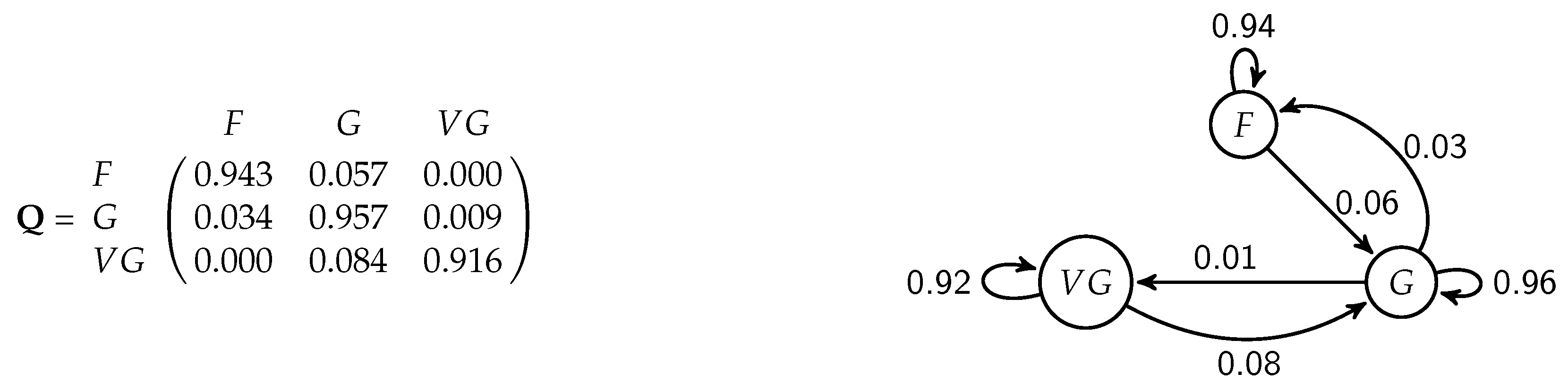Here, the labels of the hidden states will be printed in italics since such states are not observed but inferred from the data. The transition probabilities between hidden states can be represented in matrix form (Figure 2 left panel) or, since we have a relatively low number of hidden states (the latent variable has three categories in our example), as a path diagram (Figure 2, right hand side). In the diagram, the arrows corresponding to probabilities estimated as zero are not shown, and for readability purposes, transition probabilities have been rounded to two decimals.

The initial distribution of hidden state $\pi$

$$\begin{array}{cccc}& F& G& VG\\ \pi =& (0.199& 0.527& 0.274)\end{array}$$

represents the condition at baseline. Despite the overall healthy aging of the Swiss population, there is still 19.9% of chance to start the trajectory in a frail (F) state.

The limit distribution of the hidden chain

$$\begin{array}{cccc}& F& G& VG\\ (& 0.348& 0.590& 0.062& )\end{array}$$

shows a progressive decline in SRH trajectories with a probability of being in a fair condition (F) that rises to 34.8% at the end of the observational period. Nevertheless, in 59% of cases, the respondents are estimated to be in the good hidden state G.

According to the transition probabilities (Figure 2), the states are very persistent. There is more than 90% probability to stay in the same state for two consecutive periods (probabilities reported on the main diagonal of the transition matrix). Three transitions, ($F-VG$), ($G-VG$), ($VG-F$), are extremely rare or impossible. The transition probabilities for individuals with a good health condition, hidden state G, are particularly interesting. Apart from those who stay in the same hidden state, they have more chance to fall down in the frail condition (transition probability from state G to F of 3.4%) rather than to improve their situation (probability of moving from state G to state $VG$ of 0.9%).

We want to include now the effect of educational level on self-rated health trajectories of mature and older Swiss population. The level of education has been coded into three categories: (i) lower secondary level (“low”); (ii) secondary level with professional vocation (“medium”); (iii) post-secondary level (“high”). We show first the model with education at hidden level, then how to consider it at the visible level. We will use the same labels of the hidden states as in the model without covariates. However, it is worth noting that the hidden states are not exactly the same since we are including additional elements in the model. Nevertheless, looking at the response probability distribution, in our empirical example, the hidden states of the model with and without the covariate remain similar and the substantive interpretation remains the same. For simplicity then, we will keep referring to the hidden states as “fair” F, “good” G, and “very good” $VG$.

4.3. HMM with Education at the Hidden Level

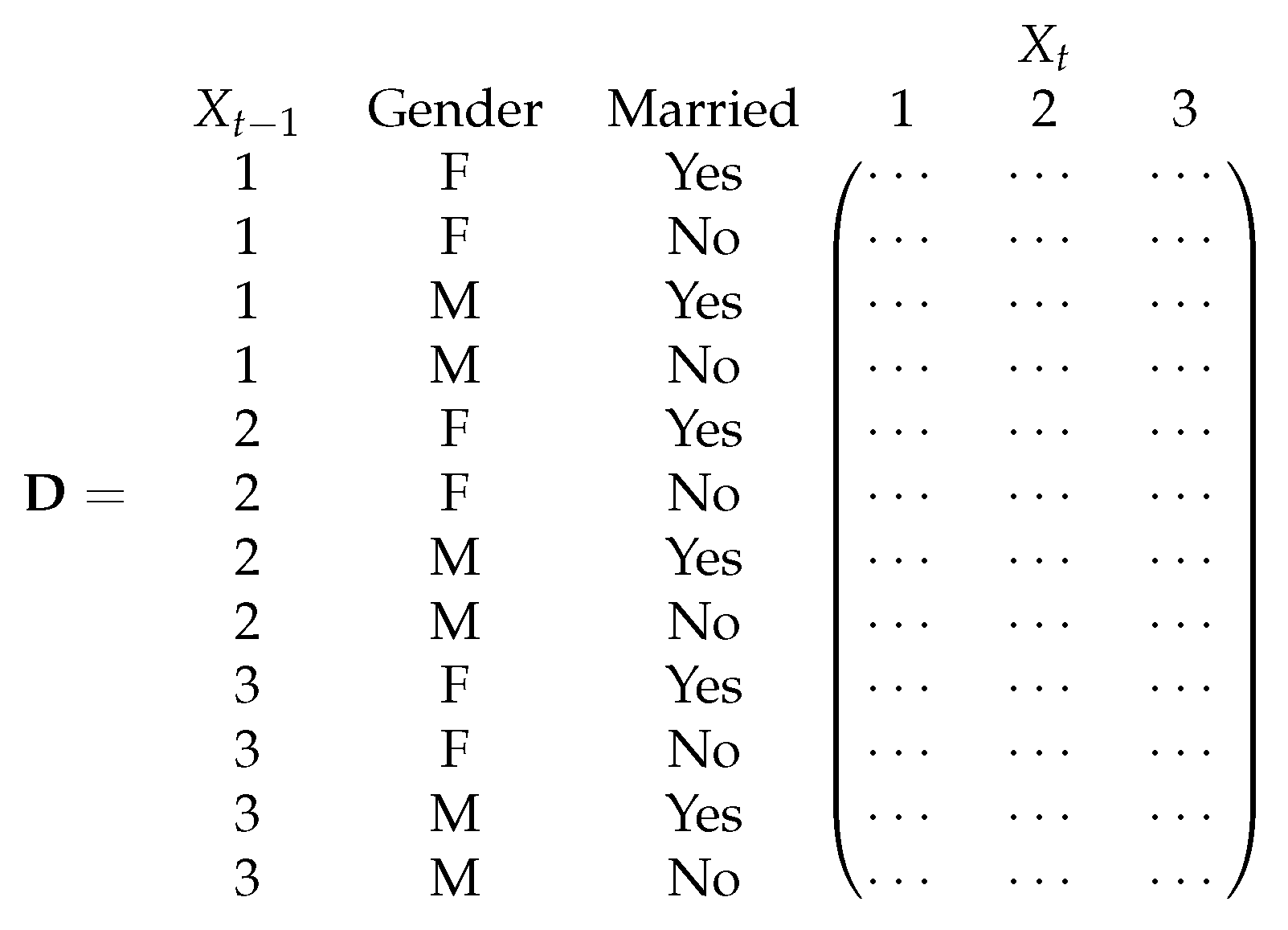
Using the 3-state hidden Markov model presented in the previous section, we include now a categorical covariate—level of education—at the hidden level. We consider both a large transition matrix with the interactions between states and levels of the covariate and the MTD-based approach.

We consider first having a unique transition matrix. The transition matrix D (Figure 3) shows a competitive advantage on health deterioration for those who have a high level of education (“High”).

The probability of falling in the hidden state F decreases with the level of education. Moreover, less educated people have a probability of being in a “fair” condition at the beginning of the sequence (initial probability distribution $\pi$), twice bigger than the most educated ones (31.1% versus 13.9%). The level of education also has a slight positive impact on chances to recover from a not-healthy condition. For instance, people with a high level of education have 2% more chance to move from a “fair” to a “good” situation (transition $F-G$) than those with a lower level of education (7.4% against 5.0% and 5.1%, respectively, for those with a medium or low educational level). Similarly, the probability of a worsening in the health condition ($G-F$) decreases with the educational attainment.

Let us consider now the MTD-based approach discussed in Section 3. We consider a mixture of the effects of the lag (transition probabilities across hidden states) and of the level of education (the response probability distribution of hidden states given the modalities assumed by the covariate). The results are reported in

Table 4. 3-state HMM model with educational level as covariate at hidden level using the MTD-based approach.

Response probability distribution. Distributions by hidden states in column.

Education	F	G	VG
Low	0.888	0.112	0.000
Medium	0.381	0.619	0.000
High	0.000	0.689	0.311

$$\begin{array}{l}\mathrm{Weight}\mathrm{parameters}\\ \mathit{\theta }=\left(0.9900.010\right)\end{array}$$

. Despite that the likelihood ratio test shows a statistically significant improvement of the likelihood (p-value for the likelihood ratio test of ≤0.005, see

Table 5. Quality of 3-state HMMs with education as covariate at the hidden level.

Covariates	Free	Log-Likelihood	BIC	p-Value Likelihood
	Parameters			Ratio Test
No covariate	20	−8893.17	17,971.8
Covariate at hidden level
Into a unique transition matrix	34	−8868.57	18,052.4	≤0.001
MTD approach	29	−8873.92	18,016.8	≤0.005

Note: Likelihood ratio test with respect to the 3-state HMM without covariates.

), the weight parameters $\mathit{\theta }$ show that the level of education has only a small effect on the latent process (it counts for only 1%). Nevertheless, as shown by the initial hidden state distribution $\mathit{\pi }$ and the response probabilities, we again observe evidence of education as a protective factor against deterioration in health. The probability of being in a frail regime (F) for instance decreases with the level of education from 88.8% for low-educated respondents to 38.1% for those with a medium level of education. Due to the low effect of education on the latent process, the transition probabilities estimated with the MTD approach for the covariate (Table 4) are similar to those estimated in the HMM without covariate ($\mathbf{Q}$ in Figure 2). The interpretation then remains the same with a stability of the states over time.

Table 5 shows the quality of the models using the two approaches. As expected, the MTD-based approach is more parsimonious and, according to BIC, performs better [32] than the model with the transition matrix made up of the interaction between the levels of the covariate and the states.

4.4. HMM with Education at the Visible Level

Let us consider now the effect of education directly at the visible level using the MTD-based approach. As before, at the hidden level we have a latent variable with three states that we will keep referring to as F, G, and $VG$. For each hidden state, the model estimates a mixture of the response probability distribution of that hidden state and the distribution of the visible SRH given the level of education. In addition, a vector of weighting parameters will be estimated to measure the relevance of the explanatory factor for each hidden state. The results of our illustrative example are reported in Table 6.

Individuals belonging to hidden state F report relatively lower levels of health with a probability of 6% of reporting a poor or bad level of health (see the response probability distribution). The respondents represented by G and $VG$ hidden states, and especially those in the latter one, are likely to be in W (well) or E (excellent) health condition. It is interesting to notice that for all three hidden states, the response probabilities show quite high values for being in a well-condition too (41.8% in F, 86.2% in G, and 54.5% in $VG$).

The weight parameters show that educational levels affect the SRH condition only for those who are in the “fair” (F) hidden state (associated weight ${\theta }_{edu}$ of 0.5451); also for them, the level of education is slightly more important to predict the current condition than the SRH itself (54.51% compared to 45.49%). For the other two hidden states, the education level has an almost null weight (0.004 for the second hidden state and 0.000 for the third hidden state). Due to the low impact of education on the data generating process, comparing the model with (Table 6) and without (Section 4.2) covariate, the initial distribution and the transition matrix of the model with and without covariate remain similar.

Since education seems to have an effect only on the first hidden state, we focus here on the results referred to F. According to the distribution of health condition by level of education, individuals in the hidden state F with a low level of education have no chance of having a good or an excellent health condition. So, education becomes more relevant in cases of poorer health, confirming the results we found including the level of education directly at the hidden level, where education plays a protective role against falling in a frail regime.

5. Conclusions

Using longitudinal data with multiple variables, it can be of interest to investigate how the current distribution of the main variable of interest depends on its previously observed values and how this dependence is moderated by external factors. The article illustrates an MTD-based approach to handle covariates in Markovian modeling. The effect of each lag and covariate is considered separately, combined by means of a mixture model. The illustrative example used a hidden Markov model with a time dependence of order one, but the proposed MTD approach for covariates can be applied to more complex Markovian models such as high-order hidden Markov models or double chains Markov models [33,34], where both the visible and latent process follow a Markovian process.

The approach discussed here has three main advantages: (i) it does not require any modification of the estimation procedure; (ii) it reduces the number of parameters to estimate with respect to a fully parametric transition matrix estimation; (iii) the weight parameters $\theta$ of the mixture model inform about the relative importance of each explanatory term. In particular, in our empirical application, we have shown that education seems to have an impact on health dynamics when we include it as an additional term in the visible model.

MTD models for not-finite state spaces have also been introduced and discussed in the literature [25,35]. The general principle of all MTD-like models for count data is to combine different Gaussian distributions using a mixture model in which the mean (and/or the standard deviation) of each distribution is a function of the past observed process. In this case, including categorical and/or continuous covariates is relatively easy and straightforward. The expectation and the standard deviation of each Gaussian distribution can be rewritten as a function of the past and of the covariates [34]. More complex is the case of a categorical outcome variable $X_t$ and a continuous covariate. In many applications, it is reasonable to partition the continuous variable into two or more mutually exclusive categories (discretization). In such a way, it is possible to directly compare the effect of each category (the levels of education in our empirical example) on the time dependence between observations. The process of discretization can be informed by the actual distribution of the covariate (i.e., looking at the distribution and then “cut” the variable accordingly, into equal intervals for instance) or by theoretical considerations. An alternative would be to use a parametrization approach and then to model directly the transition probabilities as function of the covariates. Both approaches have some drawbacks. The former can lead to arbitrary decisions on how to discretize the variable. The latter approach requires a modification of the estimation procedure, increasing model complexity. Future work should empirically investigate criteria to handle numeric covariates without increasing the complexity of the estimation procedure.