The Use of a Hidden Mixture Transition Distribution Model in Clustering Few but Long Continuous Sequences: An Illustration with Cognitive Skills Data

Abstract

In accordance with the theme of this special issue, we present a model that indirectly discovers symmetries and asymmetries between past and present assessments within continuous sequences. More specifically, we present an alternative use of a latent variable version of the Mixture Transition Distribution (MTD) model, which allows for clustering of continuous longitudinal data, called the Hidden MTD (HMTD) model. We compare the HMTD and its clustering performance to the popular Growth Mixture Model (GMM), as well as to the recently introduced GMM based on individual case residuals (ICR-GMM). The GMM and the ICR-GMM contrast with HMTD, because they are based on an explicit change function describing the individual sequences on the dependent variable (here, we implement a non-linear exponential change function). This paper has three objectives. First, it introduces the HMTD. Second, we present the GMM and the ICR-GMM and compare them to the HMTD. Finally, we apply the three models and comment on how the conclusions differ depending on the clustering model, when using a specific dataset in psychology, which is characterized by a small number of sequences (n = 102), but that are relatively long (for the domains of psychology and social sciences: t = 20). We use data from a learning experiment, in which healthy adults (19–80 years old) were asked to perform a perceptual–motor skills over 20 trials.

1. Introduction

A major goal of developmental science is to describe how individuals change in time, similarly to or differently from each other [1]. Because of natural heterogeneity in many samples, clustering methods aim at revealing groups of individuals with similar characteristics within a given cluster, but that differ from those in other clusters. Thus, clustering methods are of major importance in the study of change.

In behavioral sciences, change phenomena are often studied with growth models and similar techniques. These consist of statistical models for describing both within-person change and between-person differences that are based on mathematical change functions with interpretable parameters [2]. The parameters should allow for describing the individual trajectorie and understanding why some individuals cluster together. Individuals within the same cluster share similar, if not identical, parameter values, whereas those in different clusters are characterized by different values. The main advantage of this approach is that the nature of the parameters across the clusters can help for the substantive interpretation of the change phenomenon under investigation. Nevertheless, this approach can also yield problems, such as the overextraction of clusters [3].

Another approach to study clusters of individuals observed repeatedly consists in studying how the mathematical distribution of the dependent variable under scrutiny at a given time point depends on those at previous time points. Markovian models are typically used in this approach, because of their flexibility in terms of adjustment. In addition, Markov models have also been proposed at the latent level, where the distributional characteristics that are used for clustering are not those of the dependent variable under scrutiny, but of a latent variable thought to drive the indicator [4,5].

In this paper, we describe three different strategies to cluster longitudinal data, two of which stem from the growth model tradition and one from the Markovian approach, based on MTD model with a latent variable. The MTD model plays an important role by capturing the symmetries and asymmetries between past and present when assessing continuous sequences. We illustrate the three methods with data from a learning experiment and discuss their similarities and differences with respect to this application.

2. Data

We use a data set that was originally collected by Kennedy et al. [6] and also presented in Ghisletta et al. [7] and Ghisletta et al. [8]. The original study aimed at assessing so-called perceptual-motor skills in healthy adults with a task that requires carefully observing a visual stimulus (the perceptual component) and performing a controlled movement that follows the visual stimulus (the motor component).

2.1. Participants

The sample consisted of 102 healthy adults (19–80 years old) living in the Memphis, TN, USA, metropolitan area. The participants with sensory deficiencies and important health issues (neurological, psychiatric, and medical conditions, but also arthritis) were not included. There were 60 women vs. 42 men, and 14 African American vs. 88 Caucasians. All of the participants were right-handed and native English speakers. None were affected by dementia or by clinical depression. Concerning formal education, all attended at least high school and on average had four years of college.

2.2. Perceptual-Motor Skills

The participants underwent the Pursuit-Rotor (PR) tasks, a classical task that requires coordinating visual and motor information. The participants are seated by a rotating disk (similar to a turntable) with a hole, through which a light is vertically projected while the disk rotates. The participants hold a J-shaped wand and they are asked to keep its tip above the light as long as possible, during a 15-s trial. Twenty trials were presented with a 10-s inter-trial pause, and the apparatus measures the duration (in seconds) during which the wand is correctly kept over the light. An illustration of the entire sample of observations is provided in Figure 1, where the light lines correspond to individual trajectories, the thick black line to the average sample performance, and the red line corresponds to the expected sample trajectory according to the exponential model that we discuss below.

2.3. Other Covariates

Besides the main PR task, the participants were also assessed on a series of covariates that were thought to be potentially related to perceptual-motor skills. These include working memory tasks, which assess how well we can keep some information in mind while focusing on other information, and the capacity of cognitive adaptation. Two working memory tasks were verbal: Listening Span (LS; participants listened to simple sentences, were asked a question about their content, and finally, were asked to recall the last word of each) and Computation Span (CS; participants were to solve simple arithmetic problems and to remember the last digit of each). The two remaining working memory tasks were non-verbal: Size-Judgment Span (SJS; participants listened to a list of objects or animals and had to recall them in ascending size order) and Spatial Relations (SR; participants are presented with a whole shape as well as with a series of six disjointed shapes, from which they are asked to choose a correct combination. The complexity and degree of abstraction of the shapes augment according to participants’ capacities). The total number of correct responses was analyzed for all working memory tasks.

The Wisconsin Card Sorting (WCS) task was used to assess cognitive adaptation. In this task, the participants start by observing stimulus cards on a screen and are then shown additional cards to be singularly matched to the stimulus cards. Although no matching rules are provided, feedback about correct vs. incorrect match is provided for each card. The feedback is provided according to an existing rule, which changes during the tasks. Thus, the participants not only have to figure out the rule to correctly match cards, but they also have to adapt to a new rule, without persevering with the old one. Typically, this task is scored by counting the perseverative errors, which is, the number of matches performed by following an old rule that no longer is used for feedback. For a fuller discussion of all covariates, see Ghisletta et al. [7].

In this application, we will use these covariates to validate or invalidate our clustering solution. That is, besides discussing the interpretation of each clustering method based on the number of clusters and parameter values of each cluster, we will also investigate how the existence of the different clusters is reflected by different values in the covariates (later in Section 4).

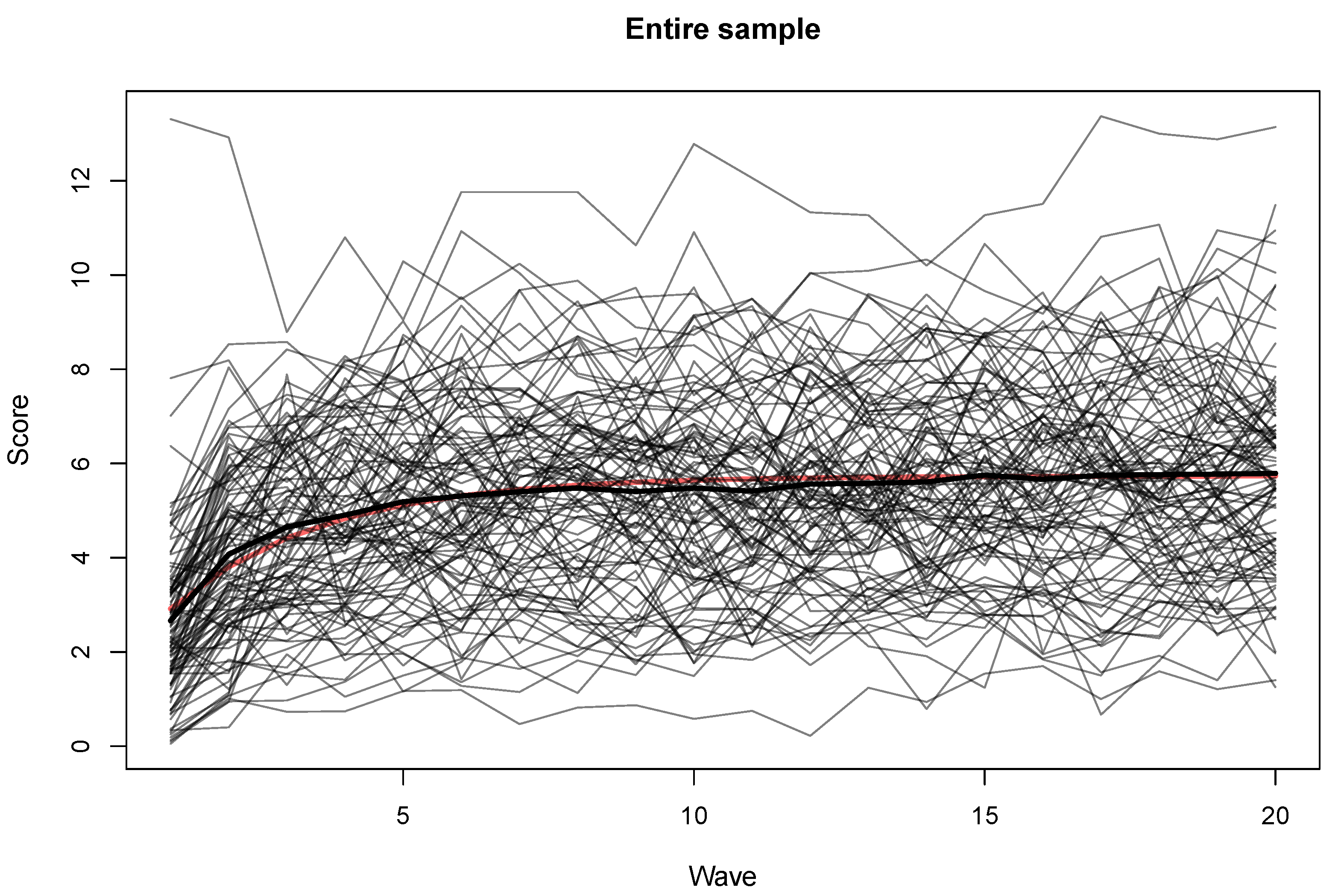
2.4. Data Characteristics and Change Functions

Before applying any clustering method, it is important to consider the data characteristics. First, this data set includes sequences that are considered to be rather long in the behavioral sciences (t = 20 trials), but on a rather small sample (n = 102). Any clustering method to be used on these data needs to account for these characteristics.

When we cluster sequences according to their average trajectory, it is very important to use a mathematical change function that adequately describes the relation between the data and time. The choice of a linear vs. non-linear function within such clustering methods has a large impact on the final results.

In Figure 1, the trajectory going through the mean values clearly suggests a non-linear time pattern for these data. The average time on target on the PR tasks has a steep slope, which corresponds to a strong learning rate, during the first 6–7 trials, and a shallower slope thereafter. The choice of an appropriate change function has been investigated in detail in Ghisletta et al. [8], who compared and tested multiple nonlinear change functions, and finally concluded that a three-parameter exponential function describes the trajectories well, as illustrated in this plot. Moreover, the exponential function is composed of parameters that are easily interpretable in terms of the learning process during the PR task. Hence, in this work, if a clustering method requires the specification of a change function, we apply the three-parameter exponential function, as specified in the following equation:

$$y_{i,t}={\beta }_i-({\beta }_i-{\alpha }_i){exp}^{-(x_{i,t}-1){\gamma }_i}+{ϵ}_{i,t},$$

(1)

where the parameter ${\alpha }_i$ represents the initial score (on the first trial), ${\beta }_i$ represents the final score (on trial 20), ${\gamma }_i$ denotes the rate of change (learning rate) for an individual i, and $x_{i,t}$ indicates the time period at each wave t (ranging from 1 to 20). ${ϵ}_{i,t}$ represents the deviation from a person’s observed score at a given time point and the model’s prediction for that score.

This model estimates a total of 10 parameters: three fixed parameters, which is, average values that describe the mean sample trajectory ($\alpha$, $\beta$, $\gamma$), six random parameters, which represent individual differences from the fixed parameters (the variance of each fixed parameter and their three covariances), and the error variance, which denotes variance of the ${ϵ}_{i,t}$ and it is typically kept constant at each time point. Thus, the rather low number of parameters makes for a change function that should not require enormous sample sizes to be estimated.

While the exponential function appears to be quite well suited to the learning-type data that we discuss here, it obviously cannot adequately describe individual trajectories stemming from any change process. The free-basis growth model is a flexible specification of the growth model that, in a spline-like manner, describes at best trajectories generated from any change process [2]. It can be written by the following equation:

$$y_{i,t}={\beta }_{0,i}+{\beta }_{1,i}·{\alpha }_t+{ϵ}_{i,t}$$

(2)

Here, ${\beta }_{0,i}$ represents the initial value for participant i at time 0, ${\beta }_{1,i}$ represents the slope, thought to be constant in time, and ${\alpha }_t$ reflects the effect of the time-invariant slope at time t. If ${\alpha }_t$ is equal to 1 at every time point, then we obtain the linear growth model, by which the individual trajectories are straight lines with constant slopes. The advantages of the free-basis model is that it is able to describe well any average linear or nonlinear trajectory. However, its main drawback is the very high number of parameters, because of the ${\alpha }_t$ parameters. In our application, this model estimates 24 parameters (two fixed and three random effects of ${\beta }_0$ and ${\beta }_1$, the error variance, and 18 ${\alpha }_t$ values—for two time points ${\alpha }_t$ needs to be fixed for identification purposes, cf. Ghisletta and McArdle [9]). Thus, the free-basis model requires large sample sizes to yield stable solutions.

The choice of a change function needs to be thorough, because, once we include a change function in a clustering method, the parameters to be estimated quickly increase. For instance, if we choose the free-basis growth model to dictate the clustering method within a GMM, then for each cluster we may have to estimate all parameters. In our case, with 20 time points, to extract two clusters we would have to estimate $2\times 24=48$ parameters. However, if we opt for the exponential function, as described in (1), we would have to estimate $2\times 10=20$ parameters to extract two clusters. Moreover, we could also choose to apply GMM with respect to only some parameters of the exponential function. If we were to let only fixed effects drive the clustering method, we would have to estimate $10+3=13$ parameters for two clusters.

To cope with this issue, we need to minimize the number of parameters by fitting the simplest possible models to the data. However, the apparent non-linearity of the data, combines with the second particularity: the relatively large number of periods (length of the sequences), which makes some more flexible models (like the free-basis growth model or high-order polynomials) very difficult to estimate with more than two clusters.

To summarize, this type of data, which is quite common in the social sciences, requires using clustering methods that are based on change functions with few parameters, but that are also able to fit well its non-linear shape. The number of parameters to estimate should also not grow considerably with the number of clusters (ex: avoid complex variance-covariance structure between clusters, over time etc.) in order to be able to include small but distinct clusters within the final partition. Flexible change functions (like the free-basis growth model or high-order polynomials) are very difficult to estimate with more than two clusters with such data.

3. Clustering Models

In this paper, we test three different methods for clustering longitudinal data: the Growth Mixture Model (GMM), a recent residual-based clustering method from Marcoulides and Trinchera [10] and the Hidden Mixture Transition Distribution (HMTD) from Berchtold and Raftery [11].

3.1. Growth Models and the Growth Mixture Model (Gmm)

Growth modeling aims to discover the patterns of (and model) individual change in a longitudinal data framework. Basic growth models assume that all trajectories belong to the same population and they may be approximated by a single average growth trajectory while using a single set of parameters. However, there exist several models, with similar assumptions, which take into account the presence of underlying (latent) groups. Such is the latent class growth analysis LCGA, which assumes null variance-covariance for the growth trajectory within each class [12], and the heterogeneity model, which imposes the same variance-covariance structure within each group of subjects. The more flexible GMM relaxes these assumptions and it will be used in our analysis.

The Growth Mixture Model (GMM) model has become a reference in the continuous longitudinal data modeling, with various applications in criminology [13], health and medicine [14,15], psychology and social sciences [16,17,18], among others (see [19]). The GMM [14,20] is a model designed to discover and describe the unknown groups of sequences that share a similar pattern. This method may be represented as a mixture of mixed-effects models, where each of the unknown sub-populations follows a distinct linear mixed effect model. Its main advantage over previous similar models is that it allows for the estimation of a specific variance-covariance structure within each class [13]. Within-class inter-individual variation is allowed for the latent variables via distinct intercept and slope variances, which are represented by a class-specific fixed effects and random effects distribution. In other words, the variation around the group-specific expected trajectory is distinct for each group, which implies heterogeneity in the growth trajectories.

In its very general form, the equation of the model for a subject i being part of class k ($c_i$ is a variable indicating to which cluster k the observation i is assigned) at time t is:

$$y_{i,t|c_i=k}=X_{1i}{\left(t\right)}^T\beta +X_{2i}{\left(t\right)}^T{\delta }^{\left(k\right)}+V_i{\left(t\right)}^T{u}_i^{\left(k\right)}+w_i\left(t\right)+{ϵ}_{i,t},$$

(3)

where $X_{1i}$ is vector of covariates with common fixed effects $\beta$, $X_{2i}$ is vector of covariates with class-specific fixed effects ${\delta }^{\left(k\right)}$, $V_i$ is a set of covariates with individual class-specific random effects $u_i^{\left(k\right)}$. Finally, $w_i\left(t\right)$ is an auto-correlated Gaussian process with null mean and covariance equal to $cov\left(w_i\left(t\right)w_i\left(s\right)\right)={\sigma }_w^{2}exp(-\rho |t-s\left|\right)$.

Initially, we attempted to use a linear change function in our example for the sake of simplicity. Thus, only time was present as random effect, no other covariate was used, and the model was estimated with the R package lcmm of Proust-Lima et al. [21]. The use of the linear function is not adapted to the data and, as expected, the results were not interpretable, as shown previously. Therefore, the focus was on the non-linear implementation of GMM, by testing the three-parameter exponential change function.

When adapted to the purpose of clustering, the coefficients of the exponential Equation (1) become specific to each cluster instead of different for every unit. Therefore, for each individual i that is assigned to cluster k, the equation of the estimated non-linear GMM with exponential trajectory becomes:

$$y_{i,t|c_i=k}={\beta }^{\left(k\right)}-({\beta }^{\left(k\right)}-{\alpha }^{\left(k\right)}){exp}^{-(x_{i,t}-1){\gamma }^{\left(k\right)}}+{ϵ}_{i,t},$$

(4)

where ${\alpha }^{\left(k\right)}$,${\beta }^{\left(k\right)}$, and ${\gamma }^{\left(k\right)}$ are the cluster-specific coefficients indicating the initial score, final score, and rate of increase. The time period $X_{i,t}$ is the only variable in the equation and it appears in a non-linear way ($X\in [1,...,T]$, where T is the last period in the data).

These coefficients follow a multivariate Gaussian distribution:

$$\begin{array}{c}\left[\begin{array}{c}{\alpha }^{\left(k\right)}\\ {\beta }^{\left(k\right)}\\ {\gamma }^{\left(k\right)}\end{array}\right]\sim \mathcal{N}\left[\begin{array}{c}\left[\begin{array}{c}{a}^{\left(k\right)}\\ b^{\left(k\right)}\\ g^{\left(k\right)}\end{array}\right],\left[\begin{array}{ccc}{\sigma }_a& .& .\\ {\sigma }_{ab}& {\sigma }_b& .\\ {\sigma }_{ag}& {\sigma }_{bg}& {\sigma }_g\end{array}\right]\end{array}\right],\end{array}$$

(5)

where the means $a^{\left(k\right)},b^{\left(k\right)}$ and $g^{\left(k\right)}$ are specific to each cluster k. However, the variance-covariance matrix is constrained to be the same over all classes, for identification purposes. Finally, the residuals are also Gaussian and their standard deviation ${\sigma }_e$ is also constrained to be the same for all of the clusters:

$${ϵ}_{i,t}\sim \mathcal{N}(0,{\sigma }_e)$$

(6)

We also attempted to relax the constraints on the variance-covariance matrix by allowing the model to have different residual standard deviations for each cluster, i.e., ${\sigma }_e^{\left(k\right)}$. This led to an increase in the number of parameters to be estimated, and it resulted in computational issues that we encountered when estimating the model with the software Mplus [22].

In the end, the exponential GMM remains inexpensive in terms of number of parameters: one residual variance ${\sigma }_e$ and six variance-covariance parameters for the coefficients from Equation (5) that are common for all groups, and three parameters for the means $a^{\left(k\right)}$,$b^{\left(k\right)}$,$g^{\left(k\right)}$ that are specific to each cluster. In other words, clusters are defined as a function of the fixed effects only of Equation (1).

3.2. Residual-Based Approach (Marcoulides and Trinchera)

Recently, Marcoulides and Trinchera [10] presented another approach to clustering longitudinal data, which was based on the individual residuals from a common growth model. Their procedure is initiated with one global growth model for the entire sample, followed by an estimation of a “local” model for each cluster separately. The idea is that, if a latent class exists in the sample, then the trajectories of the individuals belonging to that class will share similar residuals with respect to the global model and will have minimal residuals with respect to a local model estimated only within this class.

The method that is described by Marcoulides and Trinchera [10] is executed by the following steps (cf. Table 1 in Marcoulides and Trinchera [10], p. 394):

• a common growth model is fitted to the entire sample;
• individual case residuals from the common growth model are calculated;
• these residuals are clustered using a hierarchical algorithm;
• the user determines the number k of latent classes based on the hierarchical clustering dendrogram and related output;
• the individuals are assigned to one of the k latent classes;
• the k latent classes are treated separately and a common growth model is fitted to each;
• the distances between each individual sequence and each of the k local growth models are computed and compared;
• each individual is assigned to its closest local growth model (cluster);
  Steps 6 to 8 are iterated until convergence criterion is met (i.e., no more cluster switching or a maximal number of iterations); and,
• an average growth trajectory (and its parameters) for each cluster is computed.

An Euclidean type measure is used to calculate the distance between each individual and each model. It is based on the sum over time of all errors between the sequence and average pattern, predicted by the model of each cluster (individual case residuals ${ϵ}_{i,t}=Y_{i,t}-{\widehat{Y}}_{i,t}$). A drawback of this distance metric is that it only accounts for the average error, which means that sequences with completely different trends and patterns, but equal errors, end up with the same individual case residual.

Originally this method was presented using linear or free-base growth models. However, we needed to adapt the algorithm to an exponential growth model according to Equation (1), as discussed previously. Section 4 will provide the results.

Within their algorithm, the growth model is the free basis of Equation (2), and clusters are defined with respect to all of the estimated parameters. Hence, as discussed before, this approach necessitates the estimation of many parameters, which increase linearly as a function of the number of clusters to be extracted. In our application, the free-basis estimates 24 parameters per cluster, so that, for instance, the extraction of three clusters would estimate $3\times 24=72$ parameters.

We initially implemented the free-basis growth model, but, as expected, it failed to converge with more than two clusters, because of the excessively large number of parameters compared to the size of the sample. We also implemented the linear growth model, but, as expected, the solutions were not interpretable because the linear change function was not adequate. In the end, we adapted the algorithm to estimate the three-parameter exponential model of Equation (1), by allowing clusters to be extracted as a function of the fixed parameters $\alpha$, $\beta$, and $\gamma$. This approach was relatively successful, as discussed below.

3.3. HMTD

The third model we will use is the Hidden Mixture Transition Distribution model (HMTD), which has already been applied in health and social sciences [19,23]. The HMTD is a specific class of Markovian Models, which combines a latent and an observed (visible) level Bolano and Berchtold [4]. The visible level is a Mixture Transition Distribution (MTD) model, which was first introduced by Raftery in 1985 as an approximation of high-order Markov chains [24] and then developed by Berchtold [25] and Berchtold and Raftery [11]. Here, we use a Gaussian version of the MTD model, where the mean of the Gaussian distribution of the variable analyzed is a function of past observations. We tested several dependence orders for the mean of the Gaussian distributions of each component and, in the end we fixed at one, which simplifies the estimation of the means:

$${\mu }_{k,t}={\varphi }_{k,0}+{\varphi }_{k,1}{y}_{t-1},$$

where ${\varphi }_{k,0}$ is the constant for the mean of component k and ${\varphi }_{k,1}$ is the auto-regressive parameter indicating the dependence from the previous observation $y_{t-1}$. Note that, for our example, we do not include any covariates directly in the clustering model, but this could be done. We chose not to use the covariates for external validation purpose. Similarly, the variance of each component could be specified as a function of the past periods variability: ${\sigma }_{k,t}^2={\theta }_{k,0}+{\sum }_{s=1}^S{\theta }_{k,s}{y}_{t-s}^2$. Here, additionally, we tested several dependence orders for the variance and, in the end, it appeared to be sufficient to treat the variance as constant over time: ${\sigma }_{k,t}^2={\theta }_{k,0}$. Of importance, the dependence of the mean, its value, and the value of the variance vary across clusters k. Finally, the latent part of the HMTD model is a homogeneous Markov chain, where each state is associated with a different Gaussian distribution (component) at the observed level.

To use the HMTD model as a clustering tool, here we assume the hidden transition matrix to be the identity matrix, which means that an individual cannot change classes over time. However, various other specifications of the HMTD model are possible. More details regarding the specifications and the various algorithms used in the estimation of the model are provided in [5,26,27].

The advantages of this model are the small number of parameters to be estimated (only three per cluster: ${\varphi }_{k,0}$ and ${\varphi }_{k,1}$ for the mean, and ${\theta }_{k,0}$ for the variance), but also the lack of particular assumption (linear or non-liner) for the shape of the trajectory: the model only assumes that at each time t the data are Gaussian with parameter(s) dependent on the past. What distinguishes the clusters, in this particular specification, is how the mean depends on the past and how dispersed the observations are within each cluster, with respect to their expectations.

3.4. Underlying Assumptions and Distinction between the 3 Models

Small sample size (n) and a large number of periods (t) can result in a clustering problem for GMMs based on nonlinear change functions, because of the difficulty in estimation. For instance, in a free-basis growth model (cf. Equation (2)), there is an excessively large number of parameters to estimate as t increases (at least one parameter for each period and for each cluster). Combined with a small sample size, the available information may not be sufficient to reach a valid solution. However, if the data follow a specified change function (linear or not, such as exponential), the change function can be specified with a fixed-basis growth model (e.g., Equation (1)), and GMM may then be very useful.

HMTD, on the other hand, does not assume any growth trajectory, and thus does not require the user to specify an adequate change function. It only separates the sequences in terms of dependence of the past, level, and variability. This may be particularly useful in clearly non-liner data, when t is large and n is small, and where the focus of the application is not on uncovering and understanding how latent groups come about based on their trajectories.

Therefore, we can summarize the difference between these models as “trajectory-based” (all versions of GMM) vs. “distribution-based” (HMTD) clustering. In the following section, we will evaluate their performance and discuss their results.

4. Results

The residual-based method ICR-GMM was first presented by Marcoulides and Trinchera [10] using a free-basis growth model. With our data set, this model only converged with up to two clusters, because of the large number of parameters (48) needed to be estimated. Any additional cluster to be extracted would have required 24 additional parameters to be estimated, which was too many for our sample size. Even the simpler linear version of ICR-GMM, which is not adapted to the data, provides results with no more than three clusters. Therefore, the results of ICR-GMM based on free and linear basis change functions are only provided in the Supplementary Material.

Thus, below, we show the results of the ICR-GMM and of GMM based on the three-parameter exponential change function presented in Equation (1). These are the “trajectory-based” clustering methods. We also present the only “distribution-based” clustering method that we discuss here, the HMTD. For each method, we choose the optimal number of clusters using standard statistical criteria, such as AIC, BIC, adjusted BIC, and entropy (

Table 1. Fitting citeria for the results of all three models, as provided by the corresponding packages. The partitions that could not be estimated are marked with “-”. The best model according to each criterion is marked in bold.

	2 cl	3cl	4cl	5cl	6cl.
HMTD
AIC	6052.044	5921.18	5889.645	5822.483	5822.184
BIC	6073.044	5952.679	5931.644	5874.983	5885.184
nb. estimted parameters	6	9	12	15	18
GMM (exp.)
AIC	6058.933	6063.217	6053.86	6048.243	-
BIC	6095.683	6110.467	6111.616	6116.492	-
adjusted BIC	6051.462	6053.611	6042.126	6034.367	-
nb. estimted parameters	14	18	22	26	-
ICR-GMM (exp.)
AIC	6084.298	6071.239	6037.246	-	-
BIC	6136.797	6149.988	6142.245	-	-
BIC2	6073.625	6055.229	6015.9	-	-
nb. estimted parameters	20	30	40	-	-

). We also focus on the interpretability of each solution, in terms of parameter values. We first interpret the resulting clusters alone, and then also with respect to their relations with the additional covariates using Tukey’s pairwise comparison tests (Honest Significant Difference) between the clusters.

4.1. Gmm Clustering with Exponential Trajectory

With the exponential GMM method, we could estimate up to five clusters using Mplus. The optimal number of clusters according to BIC is two. However, the AIC and the adjusted BIC suggest five clusters, which is also our choice in terms of interpretability. The resulting trajectories are displayed on Figure 2. We can observe that all of the coefficients play a role in the separation of the groups: the initial ${\alpha }_k$ and the final ${\beta }_k$ scores, as well as the rates of change ${\gamma }_k$ differ across the five clusters. These differences can more easily be appreciated when we draw the average trajectory for each cluster, shown in red on Figure 2. The parameter values of the fixed effects of each cluster are shown in

Table 2. Estimated coefficients of the exponential trajectories for GMM (five cluster solution, top) and GMM based on individual case residuals (ICR-GMM) (four cluster partition on the bottom).

GMM	cl.1	cl.2	cl.3	cl.4	cl.5
cluster size	28	6	39	23	6
${\widehat{\alpha }}_k$	3.39	2.53	2.65	1.58	7.12
${\widehat{\beta }}_k$	7.41	5.55	5.72	3.37	9.36
${\widehat{\gamma }}_k$	0.58	0.14	0.37	0.50	0.17
ICR-GMM	cl.1	cl.2	cl.3	cl.4
cluster size	8	39	44	11
${\widehat{\alpha }}_k$	3.37	2.56	2.14	3.25
${\widehat{\beta }}_k$	6.18	5.53	4.95	5.69
${\widehat{\gamma }}_k$	0.17	0.69	0.47	0.42

.

Clusters 1, 3, and 4 have a rather steep initial increase, but only 1 and 3 reached high final scores. In contrast, groups 2 and 5 increased more gradually, and the latter started very high to end up with even better scores. If we interpret more, group 1 started rather low, but then adapted well and very quickly to the task; group 2 also started low, adapted slowly to the task, and then reached average performance; group 3 also started low, learned quickly, and eventually achieved a good final performance; group 4 started low, learned very little, and ended up with the worst final performance; and, group 5 started very high, improved even further, and ended up with the highest final performance. Groups 2 and 5 were the smallest, whereas group 3 was the largest.

Next, we analyze the groups with respect to their relations to the six external covariates. Several Tukey tests of differences between the groups are shown in

Table 3. Tukey tests for the difference in covariate mean levels between each pair of clusters. GMM with exponential trajectories: solutions with 2, 3, and 4 classes; p-values $<0.05$ are in bold.

GMM	2 cl.	3 Clusters			4 Clusters						5 Clusters
Exponential	2-1	2-1	3-1	3-2	2-1	3-1	4-1	3-2	4-2	4-3	2-1	3-1	4-1	5-1	3-2	4-2	5-2	4-3	5-3	5-4
Age	−8.040	4.200	8.783	4.583	9.003	6.755	−8.969	−2.248	−17.972	−15.724	16.060	9.649	6.654	−1.940	−6.410	−9.406	−18.000	−2.996	−11.590	−8.594
p-value	0.143	0.741	0.452	0.659	0.117	0.380	0.667	0.946	0.108	0.204	0.202	0.135	0.604	0.999	0.899	0.722	0.328	0.957	0.496	0.784
LS	4.216	0.105	−2.645	−2.751	−6.304	−8.683	3.213	−2.380	9.517	11.896	−15.778	−7.778	−9.778	−2.111	8.000	6.000	13.667	−2.000	5.667	7.667
p-value	0.342	1.000	0.898	0.808	0.216	0.068	0.957	0.893	0.435	0.257	0.067	0.132	0.085	0.996	0.629	0.856	0.372	0.979	0.858	0.709
CS	6.729	−1.415	−3.589	−2.174	−5.269	−4.787	15.065	0.481	20.333	19.852	−16.481	−7.037	−6.434	6.852	9.444	10.048	23.333	0.603	13.889	13.286
p-value	0.238	0.969	0.889	0.923	0.572	0.682	0.313	0.999	0.097	0.116	0.176	0.441	0.655	0.908	0.681	0.670	0.136	1.000	0.388	0.476
SJS	0.321	0.291	0.273	−0.018	−0.616	−1.267	−0.039	−0.651	0.578	1.229	−2.000	−0.744	−1.364	−0.500	1.256	0.636	1.500	−0.620	0.244	0.864
p-value	0.581	0.880	0.936	0.999	0.470	0.032	1.000	0.447	0.897	0.465	0.084	0.420	0.054	0.967	0.457	0.928	0.555	0.656	0.998	0.808
SR	0.189	−1.035	−2.411	−1.376	−1.764	−3.740	1.125	−1.976	2.889	4.865	−3.583	−1.776	−4.100	0.850	1.808	−0.517	4.433	−2.324	2.626	4.950
p-value	0.882	0.709	0.340	0.515	0.156	0.000	0.925	0.121	0.384	0.048	0.147	0.231	0.001	0.986	0.746	0.998	0.213	0.108	0.489	0.039
WCST	1.823	−5.444	0.465	5.909	11.649	10.501	2.760	−1.148	−8.889	−7.741	8.900	13.141	14.455	18.000	4.241	5.555	9.100	1.314	4.859	3.545
p-value	0.793	0.729	0.999	0.642	0.081	0.185	0.996	0.996	0.876	0.917	0.881	0.063	0.083	0.427	0.991	0.978	0.957	0.999	0.989	0.997

(for the linear version of GMM please see

Table A1. Tukey tests for the difference in covariate mean levels between each pair of clusters. Linear GMM: solutions with 2, 3, 4 and 5 groups; p-values $<0.05$ are in bold.

GMM	2 cl.	3 Clusters			4 Clusters						5 Clusters
(Linear)	2-1	2-1	3-1	3-2	2-1	3-1	4-1	3-2	4-2	4-3	2-1	3-1	4-1	5-1	3-2	4-2	5-2	4-3	5-3	5-4
Age	−5.831	2.883	−17.658	−20.541	−1.481	−2.106	−21.473	−0.625	−19.992	−19.367	0.582	−2.484	−10.740	−20.502	−3.067	−11.322	−21.085	−8.256	−18.018	−9.763
p-value	0.086	0.683	0.002	0.000	0.974	0.990	0.000	1.000	0.000	0.055	1.000	0.997	0.129	0.002	0.994	0.121	0.002	0.835	0.218	0.485
LS	2.979	−2.438	5.176	7.614	4.146	0.375	8.732	−3.771	4.586	8.357	−3.263	−3.513	1.292	4.837	−0.250	4.556	8.100	4.806	8.350	3.544
p-value	0.285	0.697	0.461	0.227	0.531	1.000	0.186	0.932	0.674	0.631	0.865	0.988	0.997	0.853	1.000	0.796	0.485	0.968	0.836	0.964
CS	1.367	−0.440	12.358	12.798	1.407	−5.284	10.901	−6.691	9.493	16.185	−2.544	−9.472	−1.806	14.750	−6.929	0.738	17.294	7.667	24.222	16.556
p-value	0.697	0.992	0.069	0.075	0.983	0.909	0.197	0.823	0.266	0.252	0.971	0.801	0.995	0.117	0.930	1.000	0.052	0.912	0.106	0.102
SJS	0.350	−0.156	1.065	1.221	0.323	−0.469	1.174	−0.792	0.851	1.643	0.053	−0.747	1.164	1.253	−0.800	1.111	1.200	1.911	2.000	0.089
p-value	0.336	0.915	0.149	0.106	0.851	0.931	0.167	0.725	0.386	0.229	1.000	0.890	0.136	0.252	0.871	0.208	0.324	0.191	0.220	1.000
SR	1.163	−0.693	1.796	2.490	0.925	−3.387	2.541	−4.312	1.616	5.929	−0.632	−4.632	0.480	1.768	−4.000	1.111	2.400	5.111	6.400	1.289
p-value	0.128	0.679	0.286	0.122	0.670	0.205	0.127	0.056	0.442	0.011	0.954	0.114	0.990	0.639	0.239	0.843	0.374	0.087	0.029	0.892
WCST	−9.469	8.597	−6.962	−15.559	−8.163	−9.010	−16.690	−0.848	−8.527	−7.679	7.389	−0.984	−4.062	−11.006	−8.372	−11.450	−18.395	−3.078	−10.022	−6.944
p-value	0.022	0.129	0.545	0.070	0.284	0.737	0.060	1.000	0.520	0.861	0.569	1.000	0.954	0.574	0.908	0.319	0.122	0.998	0.895	0.912

). Surprisingly only two differences are significant, both stemming from the variable SR, leading to the conclusion that group 4 has lower values than groups 1 and 5. The size of the groups may be a reason for the scarcity of significant results, although the important differences in scores led us to expect clearer differences. Ghisletta et al. [7] discuss the relevance of the SR covariate in the PR task. Given the spatial component of the PR task, the SR working memory, which is especially high in spatial components, is unsurprisingly associated to the learning tasks, whereas verbal or flexibility tasks are not very relevant to the task performance.

We must note that, as mentioned before, only the means of the coefficients (fixed effects) are different among the classes. Models with cluster-specific residual variances or variance-covariance matrices for the coefficients (random effects) could not be estimated because of computational issues using Mplus (probably caused by the size of the sample). This represents a limitation of the GMM approach for this type of data.

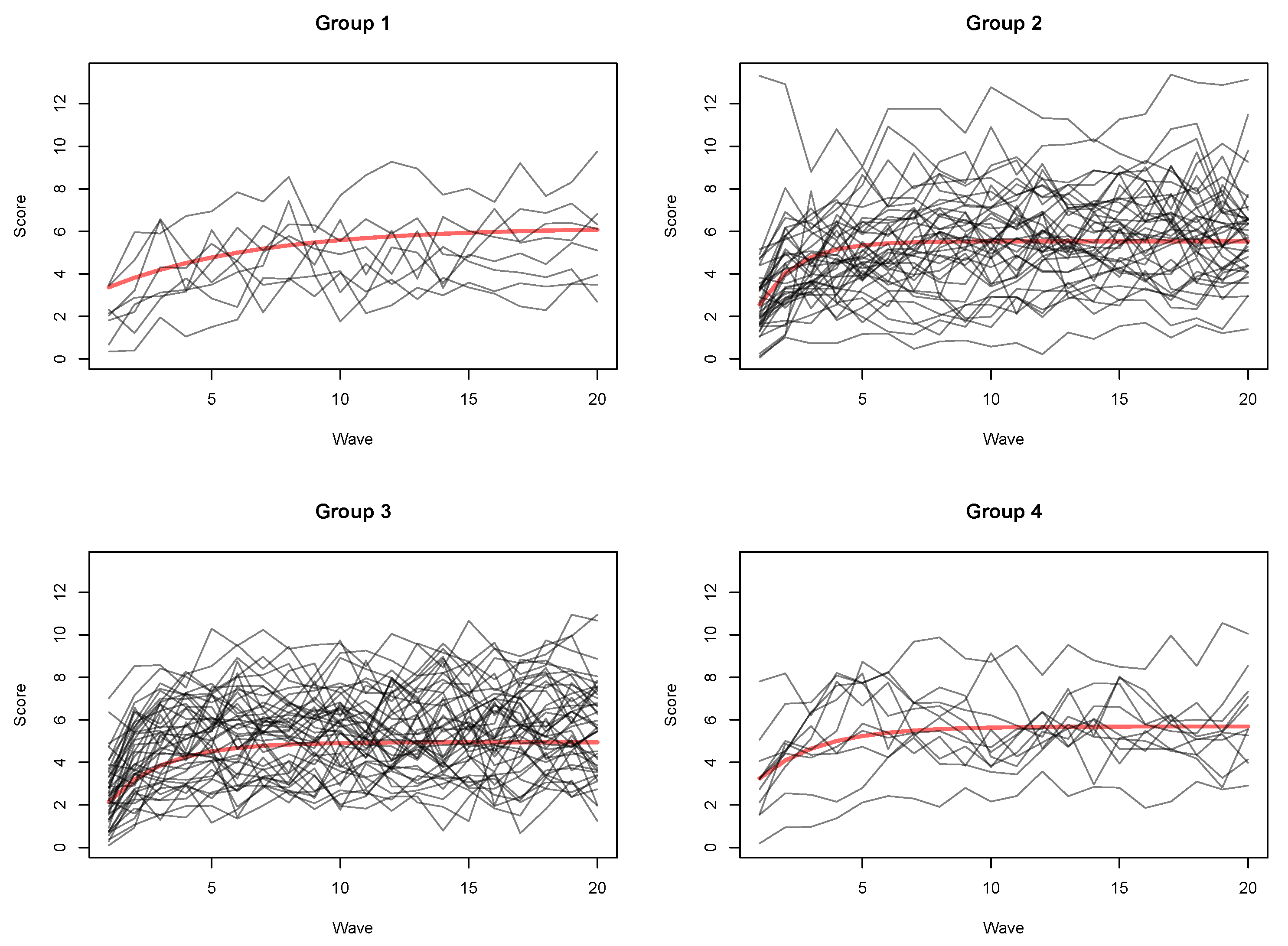
4.2. Icr-Gmm Clustering with Exponential Trajectory

We adopted the approach of Marcoulides and Trinchera [10] to fit the three-parameter exponential model, and obtained, at most, four clusters. Although BIC suggested two groups, the AIC and the BIC2, provided by the package lavaan [28], which is used in the R function provided by Marcoulides and Trinchera [10], chose the four cluster solution on which we focus. The two- and three-cluster solutions are provided in the Supplementary Material.

The partition on Figure 3 regroups four trajectories, although the differences in trajectories appear a little less important than shown by the estimated coefficients on Table 2. Clusters 1 and 4 are rather small in size (8 and 11 sequences, respectively) and they both start and finish with higher scores and a rather progressive increase. The groups 2 and 3 also share some common characteristics, such as low initial values and steeper progression. Despite these statements, we must note that the within-group variability appears rather high and the difference between groups is not as striking as it was in the previous GMM clustering.

This impression also holds when we observe the results of the Tukey tests on the covariates on

Table 4. Tukey tests for the difference in covariate mean levels between each pair of clusters. ICR-GMM method with exponential trajectories: solutions with two, three and four classes; p-values $<0.05$ are in bold.

ICR-GMM	2 cl.	3 Clusters			4 Clusters
Exponential	2-1	2-1	3-1	3-2	2-1	3-1	4-1	3-2	4-2	4-3
Age	−3.333	−4.254	−4.976	−0.723	1.240	1.648	0.625	0.407	−0.615	−1.023
p-value	0.329	0.648	0.418	0.985	0.998	0.994	1.000	1.000	1.000	0.998
LS	6.564	0.877	0.969	0.093	5.083	4.068	8.841	−1.015	3.758	4.773
p-value	0.017	0.973	0.953	1.000	0.776	0.865	0.506	0.987	0.854	0.727
CS	6.298	3.614	−0.844	−4.459	−0.868	0.655	5.614	1.522	6.481	4.959
p-value	0.071	0.749	0.977	0.591	0.999	1.000	0.891	0.980	0.687	0.822
SJS	0.040	0.234	−0.489	−0.723	0.385	0.636	0.795	0.251	0.410	0.159
p-value	0.913	0.890	0.478	0.264	0.946	0.792	0.775	0.922	0.909	0.994
SR	0.795	1.412	1.064	−0.348	1.014	1.195	2.307	0.181	1.293	1.112
p-value	0.299	0.392	0.454	0.933	0.899	0.839	0.547	0.996	0.746	0.814
WCST	−4.531	−7.583	−12.908	−5.325	10.139	9.919	5.227	−0.220	−4.912	−4.691
p-value	0.279	0.390	0.018	0.577	0.583	0.588	0.946	1.000	0.897	0.904

. There is no significant difference between the clusters on any of the covariates, which is not theoretically expected [7]. Although the average age appears higher for the group with lowest scores, the results are far from significant. Thus, it appears that, in our application, the ICR-GMM approach is not well-suited, although we adapted it with an appropriate change function.

4.3. HMTD Clustering

The last results we present in this article are those from the HMTD model (package HMTD available at https://github.com/ztau/HMTD-v0.0.1), which, in our application, focuses on the dependence of the mean scores on their past observations. Probably because of its greater computational simplicity, as compared to the GMM and ICR-GMM methods, this model allowed for the estimation of the largest number of clusters (6). The optimal number according to BIC is five, whereas AIC gives a very slight advantage to the six-group partition (Table 1). Both partitions appear very similar, with the only difference that the additional 6th cluster in the more complex solution takes its observations from clusters 2 and 5 from the five-group solution (which correspond to classes 2 and 1 in the six-cluster solution). On the correspondence matrix on Figure 4, we can see the similarity of these two partitions.

Figure 4 and Figure 5 display the trajectories of the five- and, respectively, six-cluster solution. We report the parameters for all clusters of these solutions on

Table 5. Estimated parameters for the five (bottom) and six (top side) clusters partitions of HMTD. Three groups coincide in both partitions, their correspondences are indicated on the second column of the top table.

6cl. sol.	corresp.	${\widehat{\mathit{\theta }}}_{\mathit{k},0}$	${\widehat{\mathit{\varphi }}}_{\mathit{k},0}$	${\widehat{\mathit{\varphi }}}_{\mathit{k},1}$
	5cl. sol.
1		1.81	4.81	0.53
2		1.07	4.47	0.37
3	3	0.65	1.07	0.67
4	4	1.32	2.76	0.29
5	1	1.00	3.18	0.43
6		0.98	4.13	0.51
5cl. sol.		${\widehat{\theta }}_{\mathit{k},\mathbf{0}}$	${\widehat{\varphi }}_{\mathit{k},\mathbf{0}}$	${\widehat{\varphi }}_{\mathit{k},\mathbf{1}}$
1		0.99	3.25	0.41
2		1.08	4.08	0.44
3		0.64	1.07	0.66
4		1.30	2.76	0.29
5		1.40	3.70	0.61

. We have the constant of the standard deviation ${\theta }_{k,0}$ within each cluster, the constant for the mean ${\varphi }_{k,0}$, and the auto-regressive part for the mean ${\varphi }_{k,1}$ (Remark: ${\theta }_{k,0}$ does not measure the variability between the sequences within each cluster, but the one of the Gaussian distribution component, i.e., the one around the expected mean for each period within each sequence. Here, this variability is constant over time but different across the clusters).

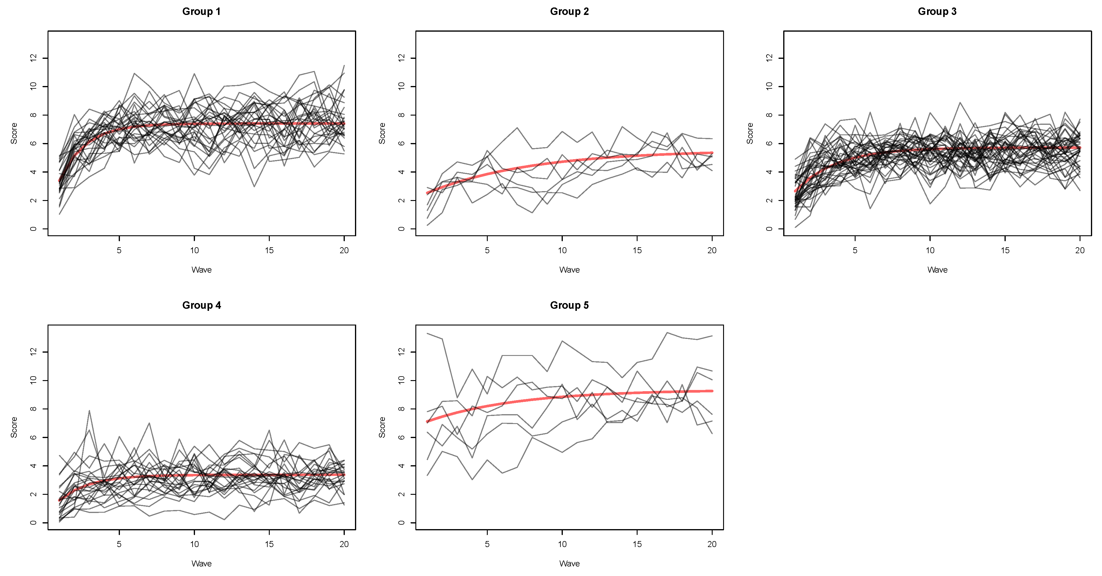
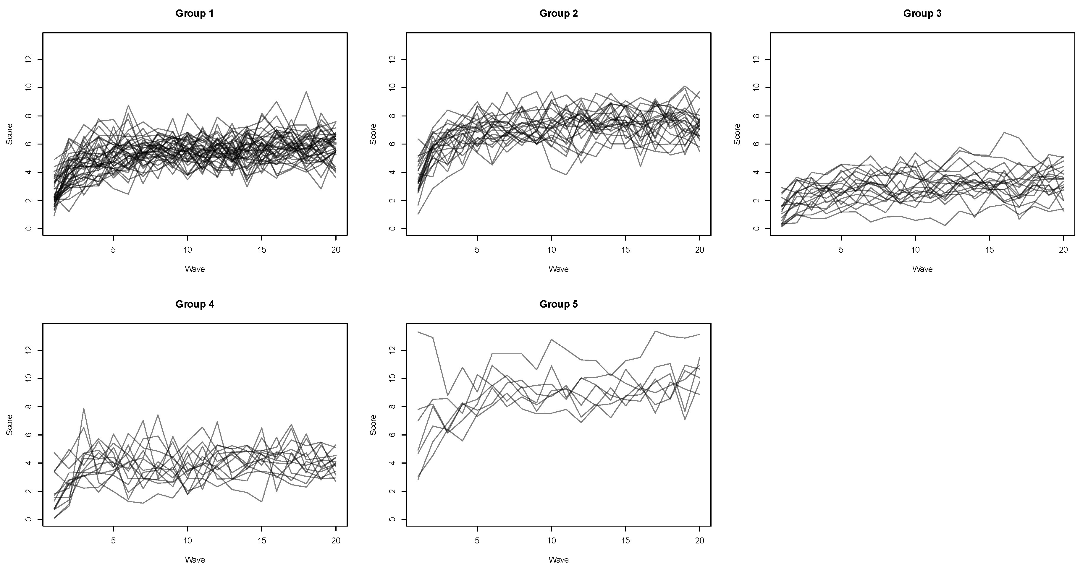
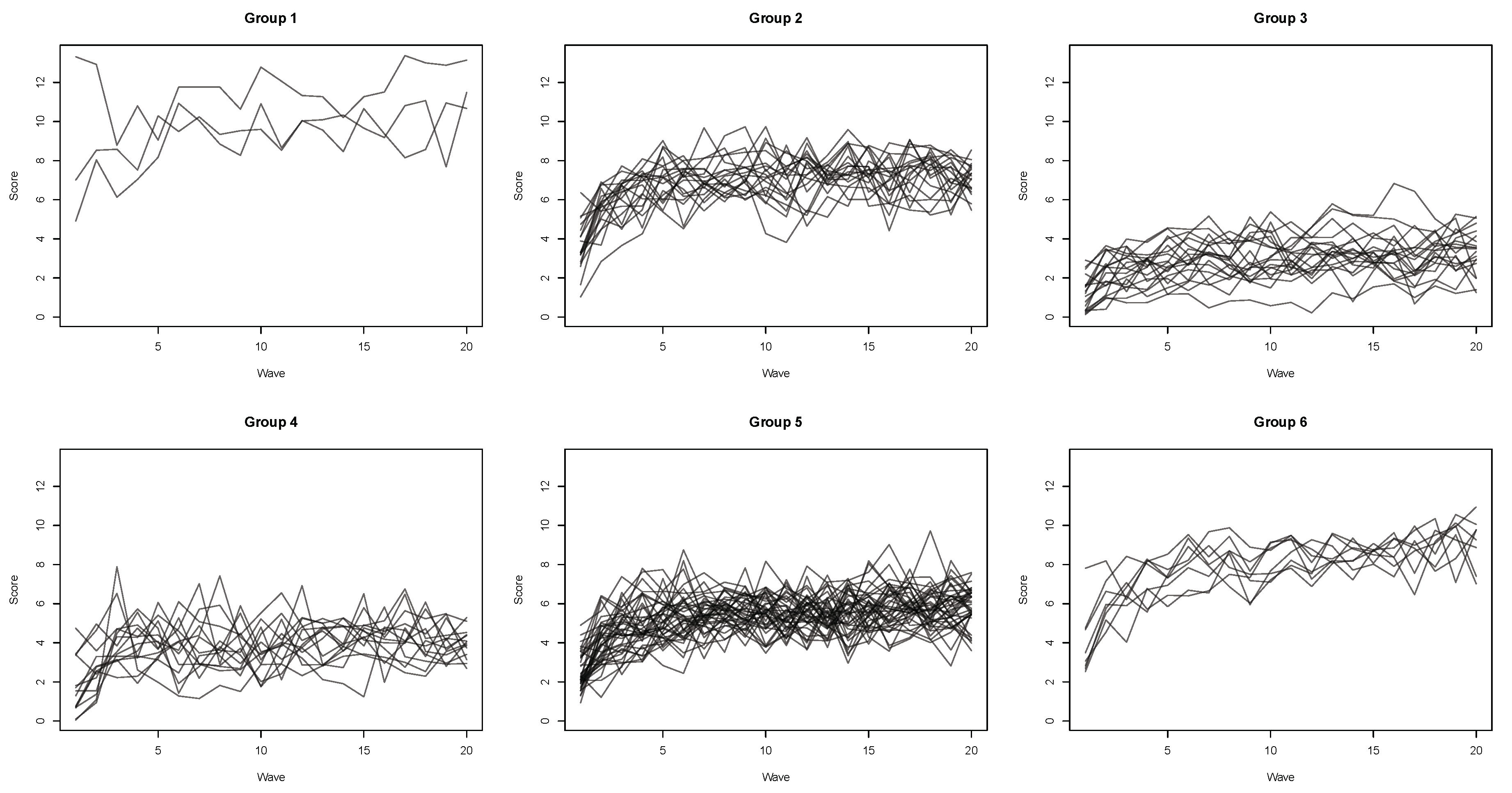
4.3.1. Five-Group Solution

The five- and the six-cluster solutions share three clusters, in which the same individuals were classified. Thus, we start by discussing these three groups. Cluster 3 (in both solutions) is characterized by the smallest constant for the mean, the largest auto-correlation, and the smallest standard deviation of all clusters. This indicates that the participants started with low scores and maintained them throughout the entire task. We call this the “lowest and stable” cluster. Cluster 4 (in both solutions) also obtained a low mean constant, but it also had a low auto-correlation and a high standard deviation. Its average performance is only slightly greater than that of cluster 3, but the sequences are much more variable over time than cluster 3 and also display a slight jump in the first three trials. We call this the “low and unstable with modest increase” cluster. Cluster 1 (which is five in the six-cluster solution) is the largest, with 39 sequences (38% of the sample), and contains the ’‘average” sequences. Its three parameters have median values as compared to those of the other clusters, and the individuals appear to display high homogeneity.

Among the clusters that are specific to the six-group solution, cluster 2 displays high constant and low auto-dependence for the mean. We call this the “normal high” performance. Finally, cluster 5 is the most erratic in terms of standard deviation. It also has high constant for the mean, and we call this the “highest and erratic” cluster.

In terms of the covariates (

Table 6. Tukey tests for the difference in covariate mean levels between each pair of clusters. HMTD: solutions with 2, 3, 4 and 5 groups; GMM with linear trajectories: solutions with 2, 3, 4 and 5 groups. p -values $<0.05$ are in bold.

HMTD	2 Cl.	3 Clusters			4 Clusters						5 Clusters
	2-1	2-1	3-1	3-2	2-1	3-1	4-1	3-2	4-2	4-3	2-1	3-1	4-1	5-1	3-2	4-2	5-2	4-3	5-3	5-4
Age	−7.882	10.581	13.187	2.606	9.756	7.267	−8.068	−2.488	−17.824	−15.336	−7.576	−1.570	9.784	−15.645	6.007	17.360	−8.068	11.353	−14.075	−25.429
p-value	0.028	0.024	0.005	0.783	0.087	0.467	0.661	0.937	0.040	0.149	0.385	0.997	0.298	0.134	0.748	0.017	0.772	0.273	0.285	0.009
LS	7.824	−3.828	−9.820	−5.992	−5.698	−8.596	3.487	−2.898	9.185	12.083	3.997	−3.620	−8.385	7.484	−7.616	−12.381	3.487	−4.765	11.103	15.868
p-value	0.008	0.472	0.014	0.158	0.343	0.176	0.931	0.850	0.326	0.179	0.787	0.871	0.284	0.641	0.372	0.066	0.973	0.858	0.332	0.087
CS	4.633	−9.217	−9.673	−0.456	−6.545	−4.809	14.026	1.737	20.571	18.835	5.831	2.175	−4.099	19.857	−3.657	−9.930	14.026	−6.274	17.683	23.956
p-value	0.215	0.074	0.067	0.993	0.400	0.776	0.195	0.979	0.012	0.048	0.676	0.990	0.935	0.032	0.953	0.407	0.276	0.823	0.112	0.019
SJS	1.202	−0.453	−1.462	−1.010	−0.570	−1.277	1.130	−0.707	1.700	2.407	0.343	−0.911	−1.000	1.473	−1.254	−1.343	1.130	−0.089	2.383	2.473
p-value	0.001	0.531	0.003	0.043	0.558	0.081	0.426	0.400	0.072	0.010	0.941	0.313	0.356	0.222	0.136	0.167	0.541	1.000	0.017	0.021
SR	2.970	−1.391	−3.800	−2.409	−1.931	−3.807	0.638	−1.876	2.569	4.444	1.388	−2.719	−1.923	2.026	−4.107	−3.311	0.638	0.796	4.745	3.949
p-value	0.000	0.237	0.000	0.016	0.136	0.005	0.979	0.217	0.333	0.044	0.549	0.063	0.419	0.671	0.003	0.055	0.994	0.971	0.039	0.153
WCST	−8.481	8.967	14.378	5.411	8.308	14.946	−5.638	6.638	−13.946	−20.583	−7.801	7.895	1.478	−13.439	15.696	9.279	−5.638	−6.417	−21.333	−14.917
p-value	0.056	0.169	0.018	0.506	0.349	0.072	0.924	0.586	0.366	0.122	0.573	0.619	0.999	0.539	0.090	0.684	0.971	0.904	0.158	0.563
HMTD	6 Clusters
	2-1	3-1		4-1	5-1	6-1	3-2		4-2	5-2	6-2	4-3		5-3	6-3	5-4		6-4	6-5
Age	7.386		10.123	21.476	11.692	−9.167		2.737	14.090	4.306	−16.553		11.353	1.570	−19.289		−9.784	−30.643		−20.859
p-value	0.973		0.902	0.269	0.811	0.953		0.994	0.121	0.921	0.134		0.319	0.999	0.050		0.347	0.000		0.012
LS	−1.982		−9.056	−13.821	−5.436	2.905		−7.073	−11.838	−3.453	4.887		−4.765	3.620	11.960		8.385	16.725		8.341
p-value	1.000		0.877	0.573	0.982	1.000		0.576	0.137	0.934	0.958		0.917	0.926	0.328		0.356	0.085		0.634
CS	−9.368		−13.111	−19.385	−15.286	0.286		−3.743	−10.016	−5.917	9.654		−6.274	−2.175	13.397		4.099	19.670		15.571
p-value	0.938		0.787	0.434	0.625	1.000		0.981	0.528	0.796	0.759		0.895	0.997	0.441		0.971	0.116		0.203
SJS	−0.368		−1.526	−1.615	−0.615	1.000		−1.158	−1.247	−0.247	1.368		−0.089	0.911	2.526		1.000	2.615		1.615
p-value	0.999		0.687	0.662	0.990	0.954		0.285	0.317	0.995	0.443		1.000	0.386	0.013		0.433	0.017		0.190
SR	−0.368		−4.412	−3.615	−1.692	0.250		−4.043	−3.247	−1.324	0.618		0.796	2.719	4.662		1.923	3.865		1.942
p-value	1.000		0.527	0.737	0.984	1.000		0.010	0.106	0.741	0.998		0.989	0.085	0.028		0.508	0.139		0.694
WCST	9.763		24.500	18.083	16.605	4.500		14.737	8.320	6.842	−5.263		−6.417	−7.895	−20.000		−1.478	−13.583		−12.105
p-value	0.985		0.554	0.834	0.853	1.000		0.207	0.860	0.817	0.988		0.949	0.711	0.168		1.000	0.658		0.614

), cluster 4 is significantly older than the clusters 2 and 5. This is coherent considering the average scores of the clusters. It is also interesting to mention that cluster 4 also has the lowest auto-correlation and, according to Figure A1 in the Appendix A, it also contains the oldest individuals on average. Cluster 5 has significantly larger CS scores than 1 and 4 and higher SJS scores than clusters 3 and 4. Thus, these individuals, who scored highest on the PR task, also had higher working memory abilities. Finally, cluster 3 (“lowest and stable”) has lower SR scores than 5 and 2.

4.3.2. Six-Group Solution

Table 7. Correspondence matrix between the five- and six-clusters solutions of HMTD.

Cluster	1	2	3	4	5	6
1	0	0	0	0	39	0
2	0	19	0	0	0	4
3	0	0	19	0	0	0
4	0	0	0	14	0	0
5	3	0	0	0	0	4

shows the correspondence matrix between the five- and six-cluster HMTD solutions and, thus, eases the comparison of these two models. As for the five-group solution, cluster 3 (“lowest and stable”) obtained the lowest constant of the mean and standard deviation, as well as the highest auto-correlation. Similarly, cluster 4 was the “low and unstable with modest increase” group, with low mean constant and low auto-correlation, but high standard deviation. Additionally, cluster 5 was the largest, and it represented the “average” group.

Cluster 1 had the highest mean constant, and it was composed of only three individuals who were in cluster 5 (“highest and erratic”) in the five-cluster solution. The remaining four individuals of cluster 5 in the 5-group solution were classified in cluster 6 here, together with four individuals previously in cluster 2. This cluster is characterized by individuals who start moderately high (but not highest) and who increase quite a bit. Finally, cluster 2 is largely similar to the previous cluster 2 “normal high” seen before.

A glance at Table 6 shows that this solution also displays some significant differences in terms of the covariates. Cluster 6 is significantly younger than 3, 4, and 5, and it also has higher SJS scores than 3. Cluster 3 has lower SR scores than 2 and 4. Although we would have expected greater group differences on the Tukey tests on the covariates, we point to the relatively small subsample sizes of each cluster, which reduces the power of the pairwise comparison test.

4.4. Correspondence between the Model Solutions

Every time that different clustering methods are applied, it is always interesting to understand the extent to which the various solutions are distinct from each other. This comparison may also guide the choice of a given clustering method over another. The correspondence matrices on

Table 8. Correspondence matrix between and the five (top) and six (bottom) cluster solutions of HMTD with the five clusters solution of exponential curve ICR-GMM (a) and exponential GMM (b).

(a)					(b)
HMTD	4 cl. exp. ICR-GMM				HMTD	5 cl. exponential GMM
5 clusters	1	2	3	4	5 clusters	1	2	3	4	5
1	3	14	17	5	1	4	2	32	0	1
2	1	9	10	3	2	20	0	1	0	2
3	1	7	9	2	3	0	2	1	16	0
4	3	6	5	0	4	0	2	5	7	0
5	0	3	3	1	5	4	0	0	0	3
6 clusters	1	2	3	4	6 clusters	1	2	3	4	5
1	0	2	1	0	1	1	0	0	0	2
2	0	7	9	3	2	16	0	1	0	2
3	1	7	9	2	3	0	2	1	16	0
4	3	6	5	0	4	0	2	5	7	0
5	3	14	17	5	5	4	2	32	0	1
6	1	3	3	1	6	7	0	0	0	1

and

Table 9. Correspondence matrix between four group exponential ICR-GMM and five cluster exponential GMM.

Exp.GMM	4 cl. exp. ICR-GMM
Clusters	1	2	3	4
1	1	9	14	4
2	0	5	1	0
3	5	15	15	4
4	2	7	12	2
5	0	3	2	1

provide interesting information about this question. The ICR-GMM method does not appear to have a clear correspondence to any of the other two methods. However, the GMM and the HMTD obtained results with this particular data set that displayed some similarities. More precisely, the five-class solutions of GMM and HMTD obtained high correspondence between clusters 1 and 2, 3 and 1, and 4 and 3, respectively.

5. Discussion

5.1. Data Particularities and Number of Parameters

The performance of a clustering method may vary highly depending on the data particularities. As mentioned, in our application we have a rather small sample size (number of sequences N), but with quite long sequences (large number of periods T). The small N reduces the power of the method and limits the maximal number of clusters that can be estimated, because a given minimal number of observations within each cluster is required for estimation. On the other hand, the increasing T requires more flexible methods of approximation and thus larger number of parameters.

What an applied researcher needs in such situations is a flexible method that remains parsimonious in terms of number of parameters to be estimated per group, yet with enough parameters for an accurate description of the data and adequate interpretation with respect to the substantive issues under scrutiny. It is also important that the method has the capacity of identifying small clusters that are truly significantly different from the others. A bootstrap approach to clustering may not be appropriate, because identical sequences may bias the estimation of the variability of the clusters, and adding noise will hinder one’s capacity to understand the behavior of the individual sequences across time.

5.2. Linearity and Trajectory Assumptions

It is common that, the longer a sequence, the less likely it is that it follows a truly linear function. As detailed, in this paper we attempted to capture the non-linearity with as few parameters as possible, by relying on previous research [7,8]. If the application calls for attention on the change function dictating the sequences, GMM and ICR-GMM might be well-suited, given that they need the explicit specification of such a change function. Additionally, analyzing the differences among the parameters across the clusters could be very useful in understanding the nature of the clusters. In our application, the learning underlying an unpracticed task (PR) lent itself to a mathematical model stipulating an initial level, and exponential acquisition rate, and a final asymptotic level of performance. However, many other sequences may stem from more random processes, so that no good guess can be made about a possible change function. Furthermore, in some cases the presence of very high volatility could make the difference between the individual trajectories vanish, which also penalizes trajectory-based methods.

Without any single clear pattern emerging in a data set, the simplicity and flexibility of HMTD may be an advantage. The lack of any precise trajectory makes the model very adaptive and economical to estimate. Moreover, this method estimates a single or possibly multiple measures of dependence from the past. The results that were obtained in this article have also shown that this method can be a very attractive alternative in such situations.

5.3. Summary of the Results

The ICR-GMM method did not provide very interesting results for this data set. Neither the trajectories in the four-cluster partition, nor their relations to the covariates appear as informative as those from the GMM and HMTD. A possible reason may be hidden in the computation of the distance considered as a sum of all the residuals across time. This calculation may underestimate the fact that some sequences may have different behavior over the different periods of time and, therefore, that their residuals may change. A residual definition that accounts for the temporality of the residuals may overcome this issue. However, we repeat that our conclusions are only relative to this particular data set.

The GMM adapted rather well to the data, mainly with the help of the exponential function. As discussed previously, the non-linear GMM could only be estimated with the same residual errors and the same variance-covariance of the coefficients among all groups. The complexity of the model made it infeasible to relax these assumptions for such a small data set and this estimation issue is a drawback of GMM. Nevertheless, it appears feasible that smaller clusters have smaller variability estimates than larger clusters, a hypothesis we were not able to test within our application.

HMTD was able to estimate the highest number of clusters here (6). As suggested by the fitting criteria, these partitions were important for the choice of the optimal number of groups. Both the five- and six- cluster solutions appear interpretable and displayed differences with respect to the covariates. Another important advantage is that this model did not require any previous information over the shape of the sequences. Here, we showed that, even in its simplest form, it adapted well to this particular data set.

6. Conclusions

Nowadays there are multiple clustering methods available to researchers of many disciplines, and interest in these applications is on a steady rise. We have limited ourselves to three methods, never before presented together, which apply to sequences of continuous data, but many other methods exist and deserve attention [4].

In this paper, we briefly discussed each of the three methods that we find particularly well-suited for sequences of continuous data: GMM, ICR-GMM, and HMTD. Each method has clear advantages, and may also present drawbacks in particular empirical settings. In our particular application, stemming from a learning experiment in cognitive psychology, the results were highly influenced by the nature of the data and the process dictating the phenomenon under investigation.

More precisely, given that we were able to apply a mathematical function that appeared to describe well the individual trajectories, the use of the GMM procedure was quite appropriate. Therefore, we suggest that, when users have strong theoretical reasons in favor of an explicit mathematical change function to describe the individual sequences, they implement this function in the GMM procedure and make use of that. If, however, there is no strong theoretical or empirical rationale in favor of an explicit mathematical function, we suggest that users apply the HMTD approach, because, given its parametric parsimony, it is quite easily estimated and it adapts well to different types of trajectories even in small samples. However, whichever method is applied, it is very important that the results be interpreted not solely based on statistical criteria, but also in light of the theoretical knowledge about the individual sequences.

It is important to stress that this work is limited to a single illustration. Clearly, additional more systematic research is needed in order to generalize the differences in behavior of these models across other types of sequences. For instance, further research could benefit from simulation experiments in which the three methods are formally compared on data generated under known underlying distributions.

References

1. Baltes, P.B.; Nesselroade, J.R. History and rationale of longitudinal research. In Longitudinal Research in the Study of Behavior and Development; Nesselroade, J., Baltes, P., Eds.; Academic Press: New York, NY, USA, 1979; pp. 1–39. [Google Scholar]
2. McArdle, J.J.; Nesselroade, J.R. Growth curve analysis in contemporary psychological research. In Comprehensive Handbook of Psychology, Vol. 2: Research Methods in Psychology; Schinka, J., Velicer, W., Eds.; Wiley: New York, NY, USA, 2003; pp. 447–480. [Google Scholar] [CrossRef]
3. Bauer, D.J. Observations on the Use of Growth Mixture Models in Psychological Research. Multivar. Behav. Res. 2007, 42, 757–786. [Google Scholar] [CrossRef]
4. Bolano, D.; Berchtold, A. General framework and model building in the class of Hidden Mixture Transition Distribution models. Comput. Stat. Data Anal. 2016, 93, 131–145. [Google Scholar] [CrossRef] [Green Version]
5. Taushanov, Z. Latent Markovian Modelling and Clustering for Continuous Data Sequences. Ph.D. Thesis, Université de Lausanne, Faculté des Sciences Sociales et Politiques, Lausanne, Switzerland, 2018. [Google Scholar]
6. Kennedy, K.M.; Partridge, T.; Raz, N. Age-related differences in acquisition of perceptual-motor skills: Working memory as a mediator. Aging Neuropsychol. Cogn. 2008, 15, 165–183. [Google Scholar] [CrossRef]
7. Ghisletta, P.; Kennedy, K.M.; Rodrigue, K.M.; Lindenberger, U.; Raz, N. Adult age differences and the role of cognitive resources in perceptual–motor skill acquisition: Application of a multilevel negative exponential model. J. Gerontol. Ser. B Psychol. Sci. Soc. Sci. 2010, 65, 163–173. [Google Scholar] [CrossRef] [PubMed]
8. Ghisletta, P.; Cantoni, E.; Jacot, N. Nonlinear growth curve models. In Dependent Data in Social Sciences Research; Springer: Berlin/Heidelberg, Germany, 2015; pp. 47–66. [Google Scholar]
9. Ghisletta, P.; McArdle, J.J. Latent growth curve analyses of the development of height. Struct. Equ. Model. 2001, 8, 531–555. [Google Scholar] [CrossRef]
10. Marcoulides, K.M.; Trinchera, L. Detecting Unobserved Heterogeneity in Latent Growth Curve Models. Struct. Equ. Model. A Multidiscip. J. 2019, 26, 390–401. [Google Scholar] [CrossRef]
11. Berchtold, A.; Raftery, A.E. The mixture transition distribution model for high-order Markov chains and non-Gaussian time series. Stat. Sci. 2002, 17, 328–356. [Google Scholar] [CrossRef]
12. Nagin, D.S. Analyzing developmental trajectories: A semiparametric, group-based approach. Psychol. Methods 1999, 4, 139. [Google Scholar] [CrossRef]
13. Francis, B.; Liu, J. Modelling escalation in crime seriousness: A latent variable approach. Metron 2015, 73, 277–297. [Google Scholar] [CrossRef] [Green Version]
14. Muthén, B.; Shedden, K. Finite mixture modeling with mixture outcomes using the EM algorithm. Biometrics 1999, 55, 463–469. [Google Scholar] [CrossRef] [PubMed]
15. Ram, N.; Grimm, K.J. Methods and measures: Growth mixture modeling: A method for identifying differences in longitudinal change among unobserved groups. Int. J. Behav. Dev. 2009, 33, 565–576. [Google Scholar] [CrossRef] [PubMed]
16. Grimm, K.J.; Helm, J.L. Latent Class Analysis and Growth Mixture Models. In The Encyclopedia of Adulthood and Aging; Whitbourne, S.K., Ed.; John Wiley & Sons, Inc.: Hoboken, NJ, USA, 2016. [Google Scholar]
17. Grimm, K.J.; Ram, N.; Estabrook, R. Nonlinear Structured Growth Mixture Models in Mplus and OpenMx. Multivar. Behav. Res. 2010, 45, 887–909. [Google Scholar] [CrossRef] [PubMed] [Green Version]
18. Muthén, B.O. Latent variable mixture modeling. In New Developments and Techniques in Structural Equation Modeling; Psychology Press: London, UK, 2001; pp. 21–54. [Google Scholar]
19. Taushanov, Z.; Berchtold, A. Markovian-based clustering of internet addiction trajectories. In Sequence Analysis and Related Approaches; Springer: Berlin/Heidelberg, Germany, 2018; pp. 203–222. [Google Scholar]
20. Bauer, D.J.; Curran, P.J. Distributional assumptions of growth mixture models: Implications for overextraction of latent trajectory classes. Psychol. Methods 2003, 8, 338. [Google Scholar] [CrossRef] [PubMed] [Green Version]
21. Proust-Lima, C.; Philipps, V.; Liquet, B. Estimation of extended mixed models using latent classes and latent processes: The R package lcmm. arXiv 2015, arXiv:1503.00890. [Google Scholar] [CrossRef] [Green Version]
22. Muthén, L.K.; Muthén, B.O. Mplus Users’s Guide, 8th ed.; Muthén & Muthén: Los Angeles, CA, USA, 1998. [Google Scholar]
23. Berchtold, A.; Surís, J.C.; Meyer, T.; Taushanov, Z. Development of somatic complaints among adolescents and young adults in Switzerland. Swiss J. Sociol. 2018, 44, 239–258. [Google Scholar] [CrossRef] [Green Version]
24. Raftery, A.E. A model for high-order Markov chains. J. R. Stat. Soc. Ser. B (Methodol.) 1985, 47, 528–539. [Google Scholar] [CrossRef]
25. Berchtold, A. Estimation in the mixture transition distribution model. J. Time Ser. Anal. 2001, 22, 379–397. [Google Scholar] [CrossRef] [Green Version]
26. Berchtold, A. Mixture transition distribution (MTD) modeling of heteroscedastic time series. Comput. Stat. Data Anal. 2003, 41, 399–411. [Google Scholar] [CrossRef]
27. Taushanov, Z.; Berchtold, A. Bootstrap Validation of the Estimated Parameters in Mixture Models Used for Clustering. J. Soc. Fr. Stat. 2019, 160, 114–129. [Google Scholar]
28. Rosseel, Y. lavaan: An R Package for Structural Equation Modeling. J. Stat. Softw. 2012, 48, 1–36. [Google Scholar] [CrossRef] [Green Version]
Figure 1. Entire sample of 102 sequences: the black curve links the mean values across all time periods and the red curve represents a fitted exponential form growth model.
Symmetry 12 01618 g001
Figure 2. Growth Mixture Model (GMM) with exponential trajectories, 5 cluster solution.
Symmetry 12 01618 g002
Figure 3. Residual-based method with exponential trajectories, four cluster solution.
Symmetry 12 01618 g003
Figure 4. Hidden Mixture Transition Distribution (HMTD) partition with six clusters.
Symmetry 12 01618 g004
Figure 5. HMTD partition with five clusters.
Symmetry 12 01618 g005