Multiple Aerodynamic Coefficient Prediction of Airfoils Using a Convolutional Neural Network

Abstract

Both symmetric and asymmetric airfoils are widely used in aircraft design and manufacture, and they have different aerodynamic characteristics. In order to improve flight performance and ensure flight safety, the aerodynamic coefficients of these airfoils must be obtained. Various methods are used to generate aerodynamic coefficients. The prediction model is a promising method that can effectively reduce cost and time. In this paper, a graphical prediction method for multiple aerodynamic coefficients of airfoils based on a convolutional neural network (CNN) is proposed. First, a transformed airfoil image (TAI) was constructed by using the flow-condition convolution with the airfoil image. Next, TAI was combined with the original airfoil image to form a composite airfoil image (CAI) that is used as the input of the CNN prediction model. Then, the structure and parameters of the prediction model were designed according to CAI features. Finally, a sample set that was generated on the basis of the deformation of symmetrical airfoil NACA 0012 was used to train and test the prediction model. Simulation results showed that the proposed method based on CNN could simultaneously predict the pitch-moment, drag, and lift coefficients, and prediction accuracy was high.

1. Introduction

Aircraft airfoils include symmetric and asymmetric airfoils. A symmetric airfoil is one with symmetrical upper and lower arcs. Typical symmetric airfoils include NACA0009 and NACA0012. To obtain better control characteristics, many horizontal tails of aircraft use symmetrical airfoils. Asymmetric airfoil is the result of deformation based on symmetrical airfoil. Generally speaking, asymmetric airfoil has a higher lift/drag ratio than symmetric airfoil does. Different airfoils have different aerodynamic characteristics that directly affect flight performance and flight safety. Therefore, the calculation of aerodynamic coefficients is an important part of airfoil design and research. Traditionally, wind-tunnel testing or computational-fluid-dynamics (CFD) simulations have been applied to obtain the aerodynamic coefficients of airfoils in the initial stage of aircraft design. However, wind-tunnel testing is not cheap in terms of cost, time, and resources, and a CFD simulation also consumes time to produce a large amount of accurate aerodynamic data.

In recent years, with the development of neural networks and machine learning, some prediction methods have been gradually applied. In these methods, prediction models that use airfoil geometric parameters and flow conditions (including angle of attack, Mach number, and Reynolds number) as input, and take known aerodynamic coefficients of airfoils as the learning object, have been established by using approaches such as kriging, multilayered perceptron (MLP), support vector machines (SVM), and support vector regression (SVR). The established models can predict unknown aerodynamic coefficients of airfoils. Thus, a large number of experiments and numerical calculations are avoided. Huang et al. [1] established a back-propagation (BP) neural-network model to predict the lift and drag coefficients of an NACA63-215 airfoil with different flow conditions. Liu [2] established a radial basis function (RBF) neural-network model to predict the airfoil lift and drag coefficients within a given parameter range. Wallach, Santos, Mattos, et al. [3,4] employed MLP and functional link networks to predict the lift and drag coefficients of NACA23012, the drag coefficients of a regional twinjet, and the drag coefficients of a wing–fuselage combination. Andrés et al. [5] hybridized an evolutionary programming algorithm with an SVR algorithm as the metamodel for the aerodynamic optimization of aeronautical wing profiles. Secco et al. [6] improved Wallach’s work [4]. There, wing–body combinations were composed of generic airfoils, and different artificial-neural-network (ANN) architectures were evaluated. In addition, the database used for ANN training suffered a considerable increase in size and number of input variables. The methods used in the above studies require geometric airfoil parameters, and are therefore called parametric prediction methods. The input data of this method are fewer, and training speed is faster when there are not many training samples. However, how to find the appropriate parameters to accurately represent airfoil geometry is the primary problem of the parametric method. Second, different airfoil-geometry representation methods use different types of parameters. It is necessary to respectively build prediction models. Third, the training time of parametric prediction methods increases exponentially with the number of samples.

Since 2006, with the intensive study of machine learning and big data, deep learning has been widely accepted and flourished [7], and has gradually been applied to the field of airfoil design. Sekar et al. [8] proposed an approach to perform the inverse design of airfoils using a deep convolutional neural network (CNN). In the training phase, the pressure-coefficient distribution was fed as input to the CNN to obtain a prediction model for the airfoil shape. In the testing phase, a new pressure-coefficient distribution was given to the CNN model, generating an airfoil shape that was very close to the associated airfoil, with an L2 error of less than 2% for most of the cases. However, only $C_p$ distribution was taken as input to CNN, which used the fixed angle of attack and Reynolds number.

In the field of the aerodynamic-coefficient prediction of airfoils, deep learning has also been applied. Yilmaz and German [9] studied a classifier based on CNN to predict airfoil performance that used airfoil images as input. The classifier predicted discrete pressure distribution on the wing surface with an accuracy of more than 80%. Zhang et al. [10] trained multiple CNN structures to predict the lift coefficient of airfoils with a variety of shapes in multiple flow conditions. One of the structures was improved on the basis of LeNet-5 [11], which processed the airfoil image to construct an artificial image as the input of the prediction model. The methods used in the above studies do not require the geometric parameters of the airfoil. Instead, they feed the airfoil images directly into the prediction model as input, and are therefore called graphical prediction methods. Compared with the parametric method, there are three advantages. First, the airfoil image can accurately represent the airfoil geometry. Second, the input of the prediction model are airfoil images and flow conditions, and no geometric parameters of the airfoil are needed. Third, the training time of the prediction model increases linearly with the number of samples.

On the basis of [12], a multiple aerodynamic-coefficient prediction method of airfoils based on CNN is proposed in this paper. This method belongs to the graphical method, but there are two differences compared with [9,10]. First, the number and types of input and output of the prediction model are different. The prediction model established in [9] was a single-input and single-output classifier. The input is the airfoil image at a zero angle of attack, and the output is discrete pressure distribution. The prediction model established in [10] was a multi-input and single-output regression. The input includes the airfoil image and flow condition, and the output is only the lift coefficient. The prediction model established in this paper is a multi-input and multioutput regression. The input is the same as [10], but the output includes three aerodynamic coefficients: pitch-moment ($C_{mz}$), drag ($C_D$) and lift ($C_L$) coefficients. Second, the way that it uses the flow condition to process the airfoil image is different than when preparing the input of the prediction model. A fixed flow condition was employed in [9], and the airfoil image was not processed. In [10], the airfoil image was tilted by the corresponding angle of attack, and colored by the free-stream Mach number and pixel density. An artificial image was constructed as the input of the prediction model. In this paper, the airfoil image was convolved with the flow condition to generate a transformed airfoil image (TAI). A composite airfoil image (CAI) was constructed as the input of the prediction model by combing TAIs and the original airfoil image. This process can keep the basic shape of the airfoil in the TAI, and it is comfortable for the CNN to extract image features.

This paper is structured as follows: the next section details the steps to establish the prediction models. Then, a simulation example is given to train and test the CNN model. Finally, a concluding section closes the paper.

2. Methodology

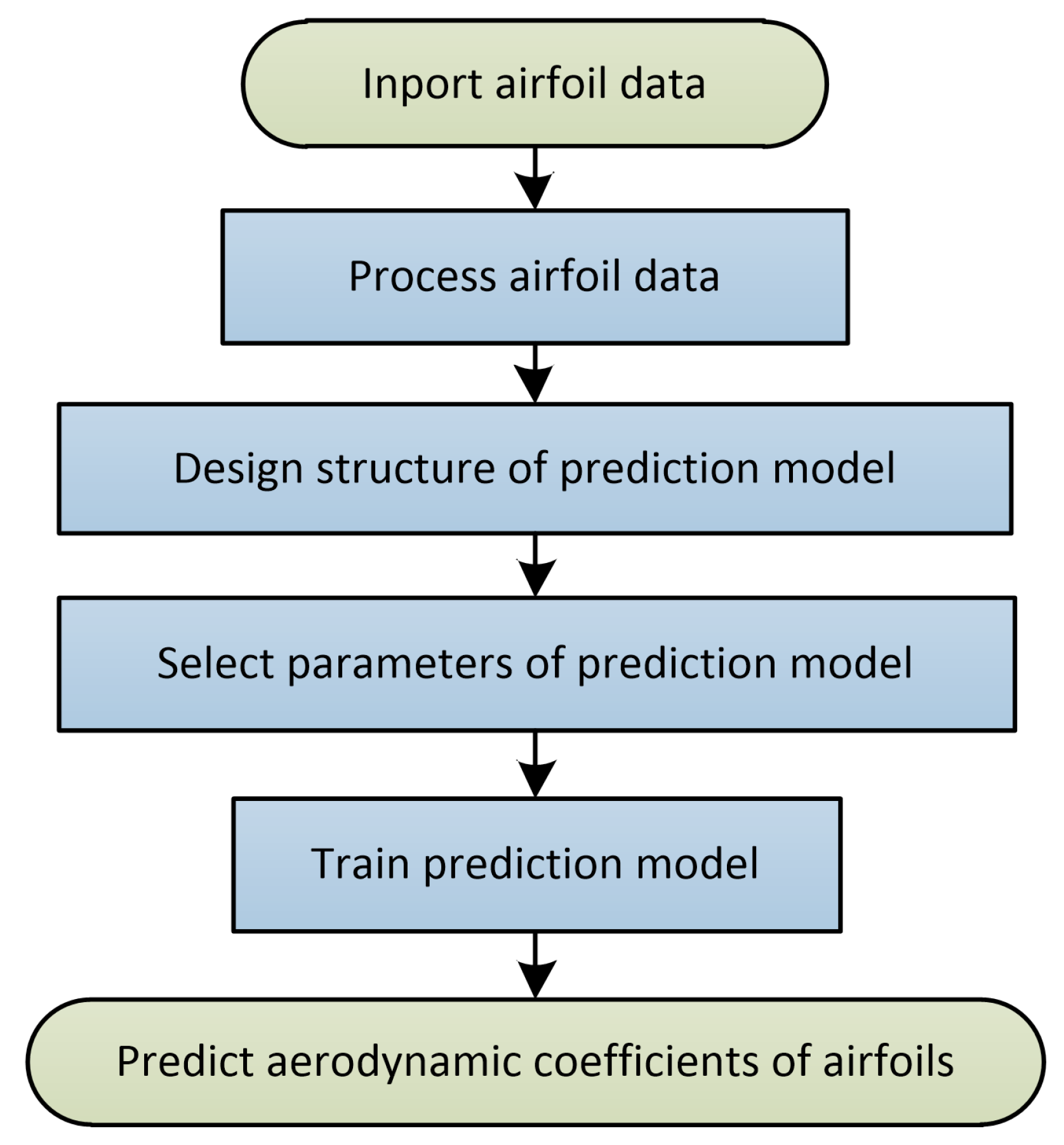
The steps to establish the aerodynamic-coefficient prediction model of airfoils are shown in Figure 1: airfoil-data processing, structure design, parameter selection, and model training.

2.1. Airfoil Data Processing

Airfoil data in this paper are flow conditions, aerodynamic coefficients, and airfoil images. The main contents of airfoil-data processing include:

(1) Defining flow-condition zoom factor.

Flow conditions include three parameters: angle of attack, Mach number, and Reynolds number. However, the order of magnitude of the parameters is quite different. If they are directly used to establish the prediction model, prediction accuracy is reduced. Therefore, they have to be adjusted by the zoom factor to ensure that the TAI and the original airfoil image have the same range of values.

(2) Normalization of aerodynamic coefficients.

The aerodynamic coefficients of airfoils include the pitch-moment, drag, and lift coefficients in this paper. The three coefficients also have differences in symbols and orders of magnitude. Therefore, it is necessary to adjust the numerical range of aerodynamic coefficients by normalization.

(3) Preparing input images.

Preparing the input images is the key to processing airfoil data. The input of the CNN prediction model is usually an image, a two-dimensional matrix for grayscale images, and three two-dimensional matrices for color images. The airfoil image was a grayscale image in this paper and could be directly used as the input of the CNN model. In general, the airfoil was flat, and its thickness and length often differed by an order of magnitude. Therefore, the thickness of the airfoil was magnified 10 times to improve the prediction accuracy of the model.

The flow conditions are three numerical parameters that could not be directly used as the input of CNN prediction model. Therefore, they had to be converted into images to be recognized. The conversion method of this paper was as follows: the airfoil image was convolved with the respective flow conditions to generate some new images, the TAIs; the combination of the TAIs and the original airfoil image (CAI) was the input to the CNN prediction model. The advantage of this method is that flow conditions were integrated into the airfoil image, and features of the airfoil image were maintained.

(4) Preparing training and test sets

The airfoil was grouped and scrambled. About 80% of the data were selected as the training set to establish the prediction model, and the remaining part formed the test set to validate.

2.2. Structure Design

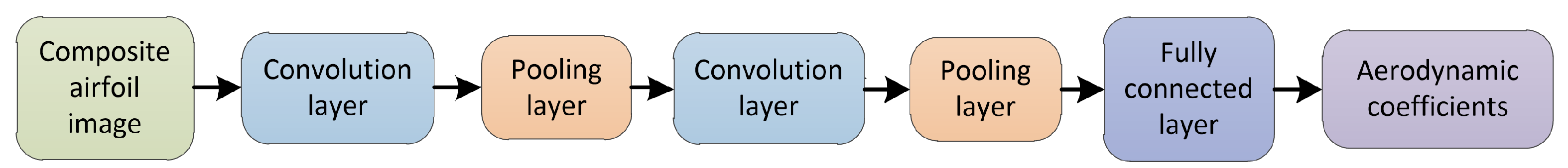
The structure of the prediction model established in this paper is similar to that of LeNet-5, as shown in Figure 2. However, the difference is that the nonlinear activation function was changed from a sigmoid to a rectified linear unit (ReLU) [13] because of its faster convergence rate. The output layer was changed from a classifier using the softmax function to a regression using the mean-squared-error (MSE) function. Since the CAIs are grayscale images, only two convolutional and pooling layers were used, which effectively prevented overfitting while ensuring prediction accuracy and training speed.

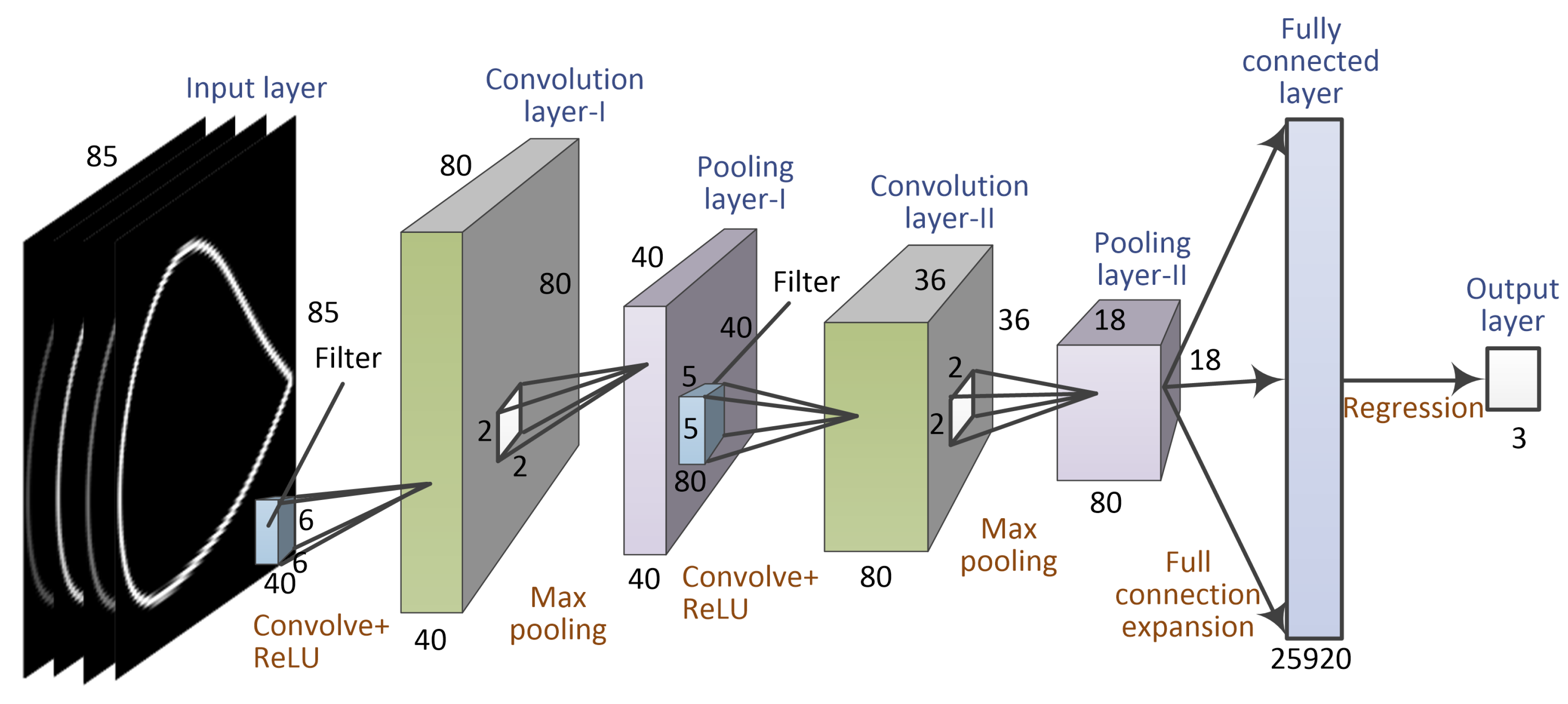
2.3. Parameter Selection

The parameters of the airfoil–CNN prediction model are called hyperparameters, and their values are shown in Figure 3.

(1) Input layer

The data of the input layer were the CAI, including TAIs and the airfoil image. In this paper, CAI resolution was set to $85\times 85$, that is, four $85\times 85$ two-dimensional matrices ranging from 0 to 255.

(2) Convolutional layer I

The convolutional layer is a core component of a CNN. Different filters can be used to obtain different CAI features. Convolutional layer I had a filter size of $6\times 6$, a filter number of 40, and a step size of 1 in each direction. After convolution and a ReLU operation, 40 feature maps with a resolution of $80\times 80$ were obtained.

(3) Pooling layer I

In order to reduce the amount of computation and prevent overfitting, a pooling layer (also called the downsampling or subsampling layer) was connected behind the convolutional layer. In general, the pooling methods of the pooling layer include average and maximal pooling. Average pooling averages the pixel values in the pooling region; maximal pooling takes the maximal pixel value in the pooling region.

Pooling layer I had a pooling size of $2\times 2$ and a step size of 2, which meant that adjacent pooling regions did not overlap. The pooling method selected maximal pooling. After pooling, 40 feature maps with a resolution of $40\times 40$ were obtained.

(4) Convolutional layer II

Convolutional layer II had a filter size of $5\times 5$, a filter number of 80, and a step size of 1. After convolution and a ReLU operation, 80 feature maps with a resolution of $36\times 36$ were obtained.

(5) Pooling layer II

Pooling layer II had a pooling size of $2\times 2$ and a step size of 2. The pooling method selected maximal pooling. After pooling, 80 feature maps with a resolution of $18\times 18$ were obtained.

(6) Fully connected layer

The number of neurons in the fully connected layer depended on the resolution and number of the feature maps in pooling layer II. In this paper, one fully connected layer with 25,920 neurons was set.

(7) Output layer

The regression output layer used MSE as the loss function to predict the aerodynamic coefficients of the airfoils. The MSE calculation formula is:

$$MSE={\displaystyle \sum _{j=1}^{s_{batch}}}\frac{{\left({\displaystyle \sum _{i=1}^{n_{coeff}}}\frac{{(y_i-x_i)}^2}{n_{coeff}}\right)}_j}{s_{batch}}$$

(1)

where $x_i$ and $y_i$ are the ith actual and predicted aerodynamic coefficient, respectively; $n_{coeff}$ is the number of airfoil aerodynamic coefficients to be predicted; and $s_{batch}$ is the minibatch size, that is, the number of CAI samples that were fed into the prediction model for each training iteration.

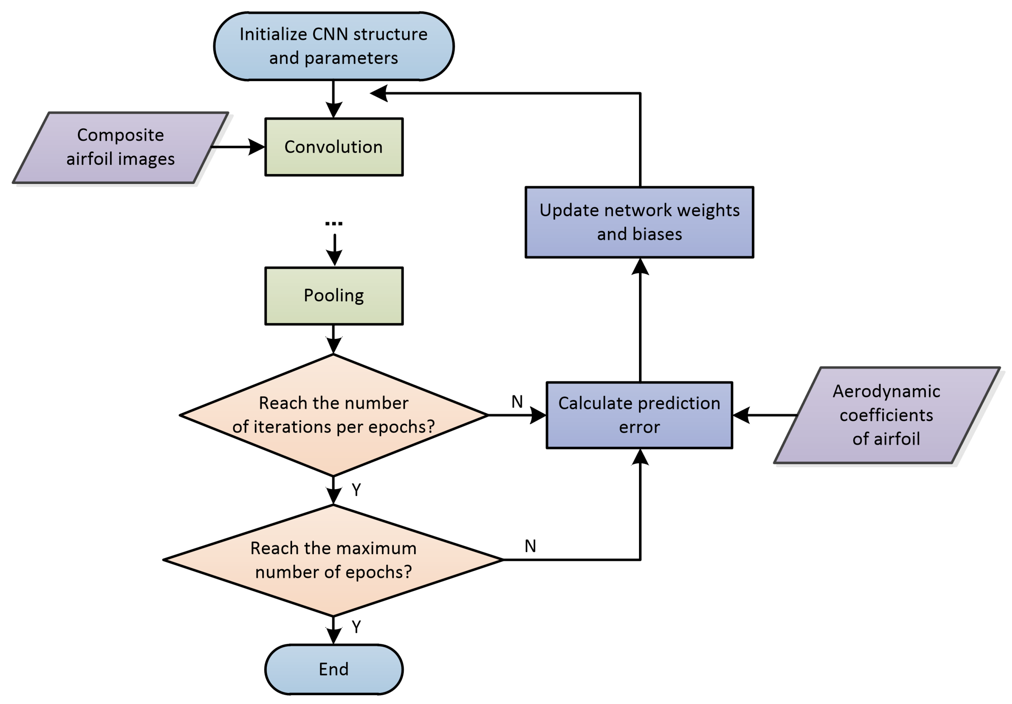
2.4. Training Process

The training process of the prediction model included two steps: forward calculation and error back propagation. Forward calculation extracted image features with the convolutional and pooling operations, constructed a conventional neural network with the fully connected layer, and obtained prediction values through the output layer. Differences between prediction and actual values were prediction errors. Error back propagation transferred prediction errors backward by the algorithms such as gradient descent, and updated network weights and biases. Depending on the complexity of the problem, the number of convolutional, pooling, and fully connected layers could be flexibly selected.

After forward calculation and error back propagation, if the end condition was not reached, the above steps were repeated. Whether the end of CNN training was achieved could be determined by the error threshold or the maximal number of epochs. In this paper, the latter is used as the end condition. The training process of the airfoil–CNN prediction model is shown in Figure 4.

In this paper, the training algorithm selected stochastic gradient descent with momentum (SGDM) [14]. An iteration was one step taken in the SGDM towards minimizing the loss function using a minibatch, which is a subset of the training set that was used to evaluate the gradient of the loss function and update the weights. An epoch is the full pass of the training algorithm over the entire training set.

3. Results and Discussion

3.1. Data Preparation

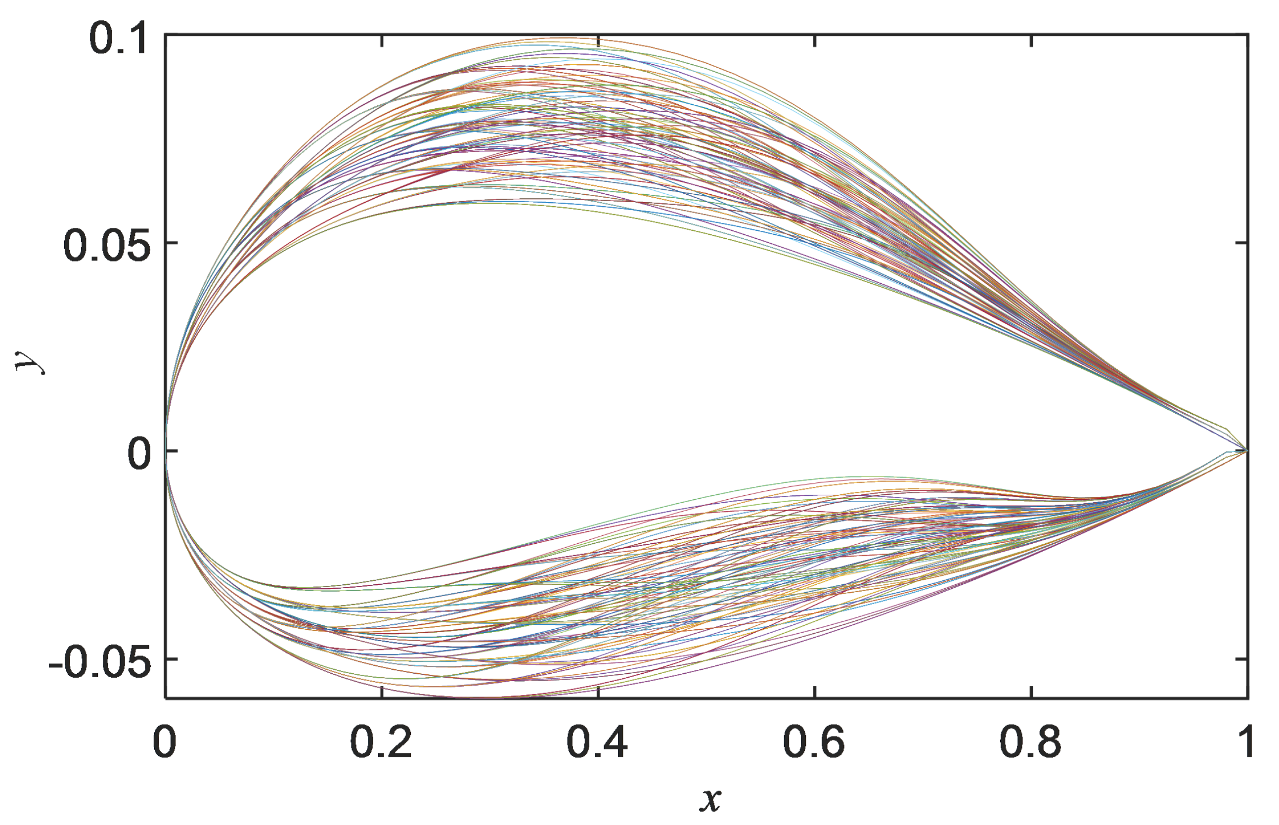
Data preparation is an important task in machine learning. The sample set of airfoils used in this study included symmetric and asymmetric airfoils. They were generated on the basis of symmetric airfoil NACA0012 through the improved Hicks–Henne bump function [15]. The number of bump function of the airfoil’s upper and lower surface were both set to 4; the values of the control points were 0, 0.005, and 0.01. A total of $3^8=6561$ 2D airfoil geometries were obtained, and 300 airfoils were randomly selected to calculate the aerodynamic coefficients under different flow conditions as the sample data of the CNN prediction model. The geometry of the 300 airfoils is shown in Figure 5.

The aerodynamic coefficients of those airfoils were calculated by computational fluid software MBNS2D [16], independently developed by our department. A Navier–Stokes (NS) equation, Roe scheme, and a two-equation k-$\omega$ SST turbulence model were adopted for this simulation. With regard to flow conditions, the angle of attack was 2, 6, 9, 12, and 15 deg; the Mach number was 0.1, 0.3, and 0.6; the Reynolds number took a fixed value of $6.5\times {10}^6$. 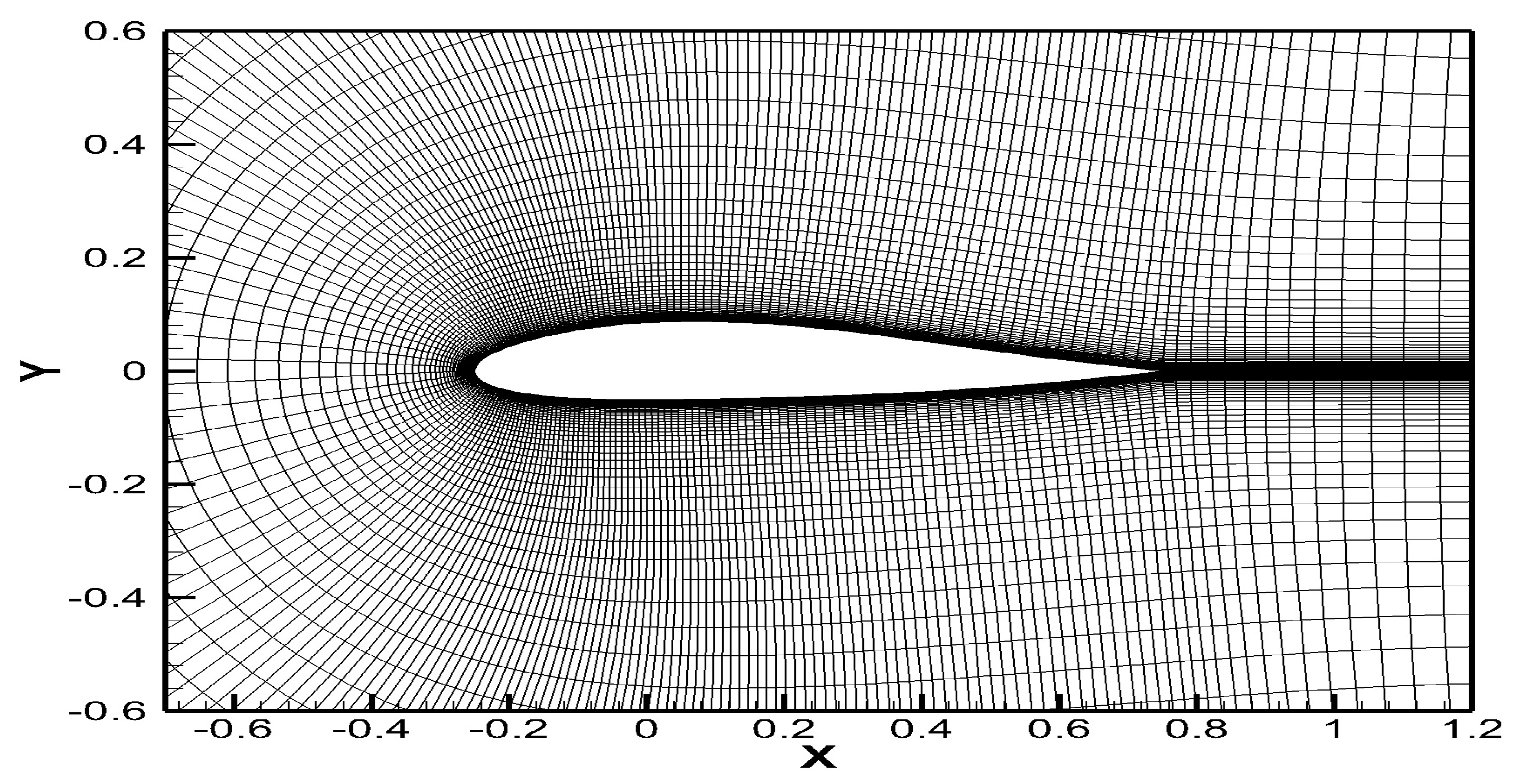Figure 6 shows the X–Y plane of the computational grid. The number of grids was set to $300\times 100$, the grids of leading and trailing edges were encrypted, and the first layer height in the wall-normal direction was less than ${10}^{-5}C$ (C is chord length). To study gird convergence, four grid levels were chosen, and the grid-refinement ratio was $\sqrt{2}$.

Table 1. Computational-fluid-dynamics (CFD) results of $C_D$ and $C_L$ ($\alpha$ = 2, Ma = 0.4, Re = $6.5\times {10}^6$).

Grid	${\mathit{C}}_{\mathit{m}\mathit{z}}$	$\mathit{ϵ}(\%)$	${\mathit{R}}_{\mathit{G}}$	${\mathit{C}}_{\mathit{m}\mathit{z}}$	$\mathit{ϵ}(\%)$	${\mathit{R}}_{\mathit{G}}$
gird1 ($210\times 70$)	0.01088	9.46		0.34306	1.2
gird1 ($300\times 100$)	0.01028	3.42	0.42	0.34443	0.8	0.53
gird1 ($420\times 140$)	0.01003	0.9		0.34516	0.6
gird1 ($600\times 200$)	0.00994	-	-	0.34740	-	-

shows the simulation results of $C_D$ and $C_L$ at a fixed-flow condition.The relative error of Grid 2 was 3.42% and 0.8%. The convergence ratio RG of Grids 1, 2, and 3 was 0.42 and 0.53. 0 < $R_G$ < 1 indicates that simulations were monotonically convergent [17]. For setting flow conditions, the Mach number and angle-of-attack values were within the normal flight speed and angle control range of an ordinary aircraft, and the aerodynamic characteristics of the aircraft in this range were approximately linear, so that the robustness of the model would not be significantly affected by the selection of samples. If the angle of attack continued to increase beyond the stall angle of attack, or the Mach number approached or exceeded 1, the flow phenomenon would become extremely complex, and the aerodynamic characteristics of the aircraft would show strong nonlinear characteristics. This belongs to special research fields, such as nonlinear problems at a high angle of attack, and transonic or supersonic flow problems.

It takes about 350 s to calculate the aerodynamic coefficients of an airfoil under certain flow conditions with a personal computer (Intel Core i5-8250U CPU, 8 GB memory, and GeForce MX150 graphics card). Airfoil geometries were grayed to obtain airfoil images. The arbitrary combination of 300 airfoil images, 3 Mach numbers, and 5 angles of attack, together with aerodynamic coefficients, could form 4200 samples (excluding aerodynamic coefficients with a 15 deg attack angle and Mach number of 0.6). The order of the 4200 samples was scrambled, and 3360 samples were randomly selected to train the prediction model where airfoil aerodynamic coefficients were used as labels. The remaining 840 samples were used as the test data to validate the prediction model.

3.2. Model Training

Since the Reynolds number takes a fixed value, it is not used to generate the TAI, that is, it does not participate in the training of the prediction model. The airfoil image is grayscale, and the corresponding two-dimensional matrix ranged from 0 to 255. TAI value should also be approximately in the same range. Therefore, the zoom factors of angle of attack and the Mach number were set to 1/16 and 25/16, respectively.

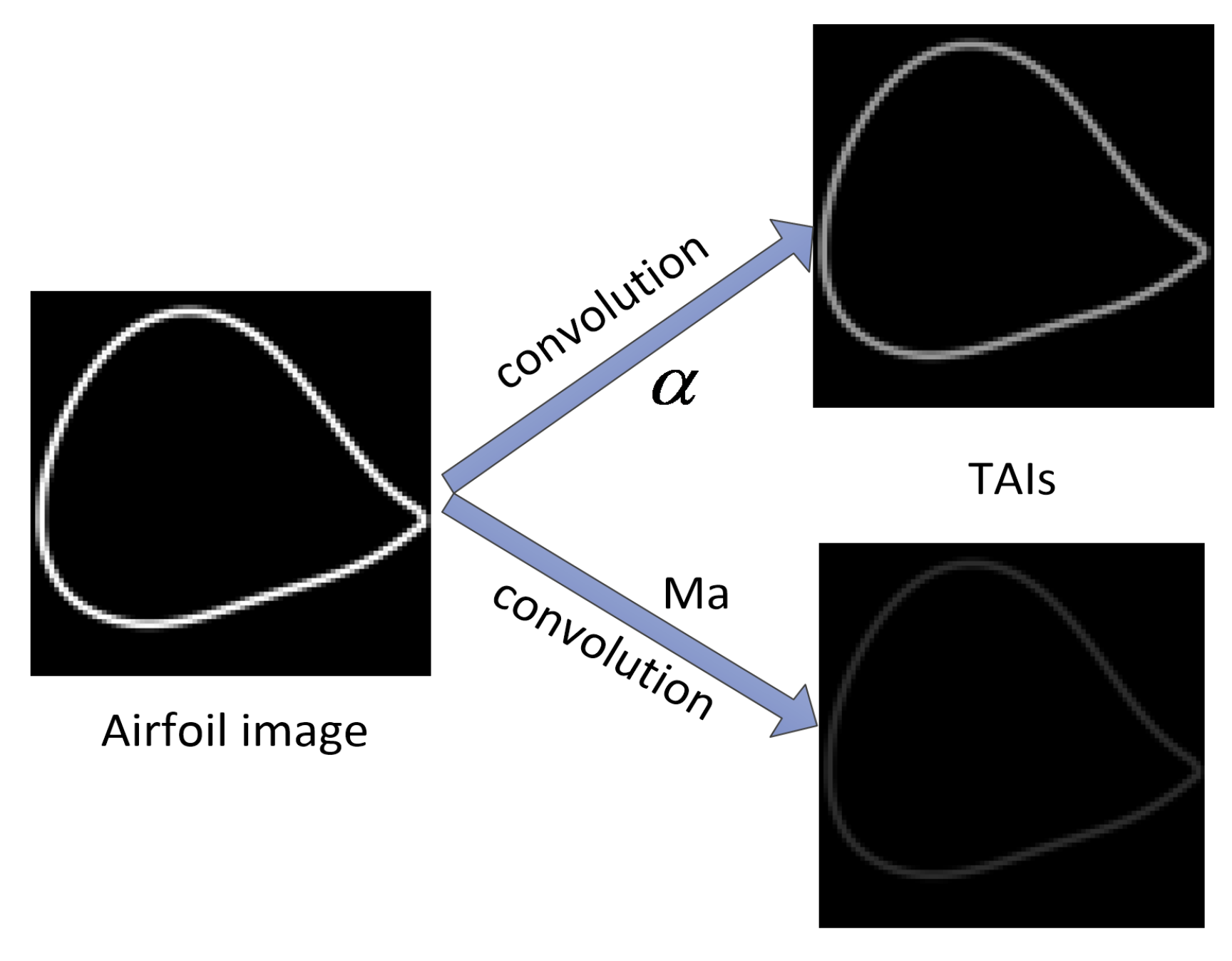
The airfoil image convolved with the angle of attack and the Mach number, respectively, to generate two TAIs. For example, a random airfoil image is shown on the left side of Figure 7. The angle of attack was 9 deg, and the Mach number was 0.1. They were multiplied by zoom factors to yield 0.65629 and 0.15625 deg, respectively. The generated TAIs by convolving them with the left airfoil image are shown on the right side of Figure 7.

The training parameters of the prediction model were as follows: momentum parameter, 0.9; minibatch size, 8, that is, eight CAIs were input in each iteration for training; maximal number of epochs, 80; the initial value of learning rate, $1\times {10}^{-6}$, which was adjusted to 70% every 6 epochs; $L_2$ regularization parameter, $1\times {10}^{-4}$. It cost about 35 minutes to train the model with the same personal computer. The training time of the model was closely related to the number of training samples. However, If the number of samples were maintained, only the sampling points of the design variable were changed, e.g., angle of attack was set to 2, 5, 8, 11, and 15 deg; it would have little effect on the training time of the model, and on the prediction capability of the model, as aerodynamic characteristics were approximately linear within this angle of attack‘s value ranges, as mentioned above.

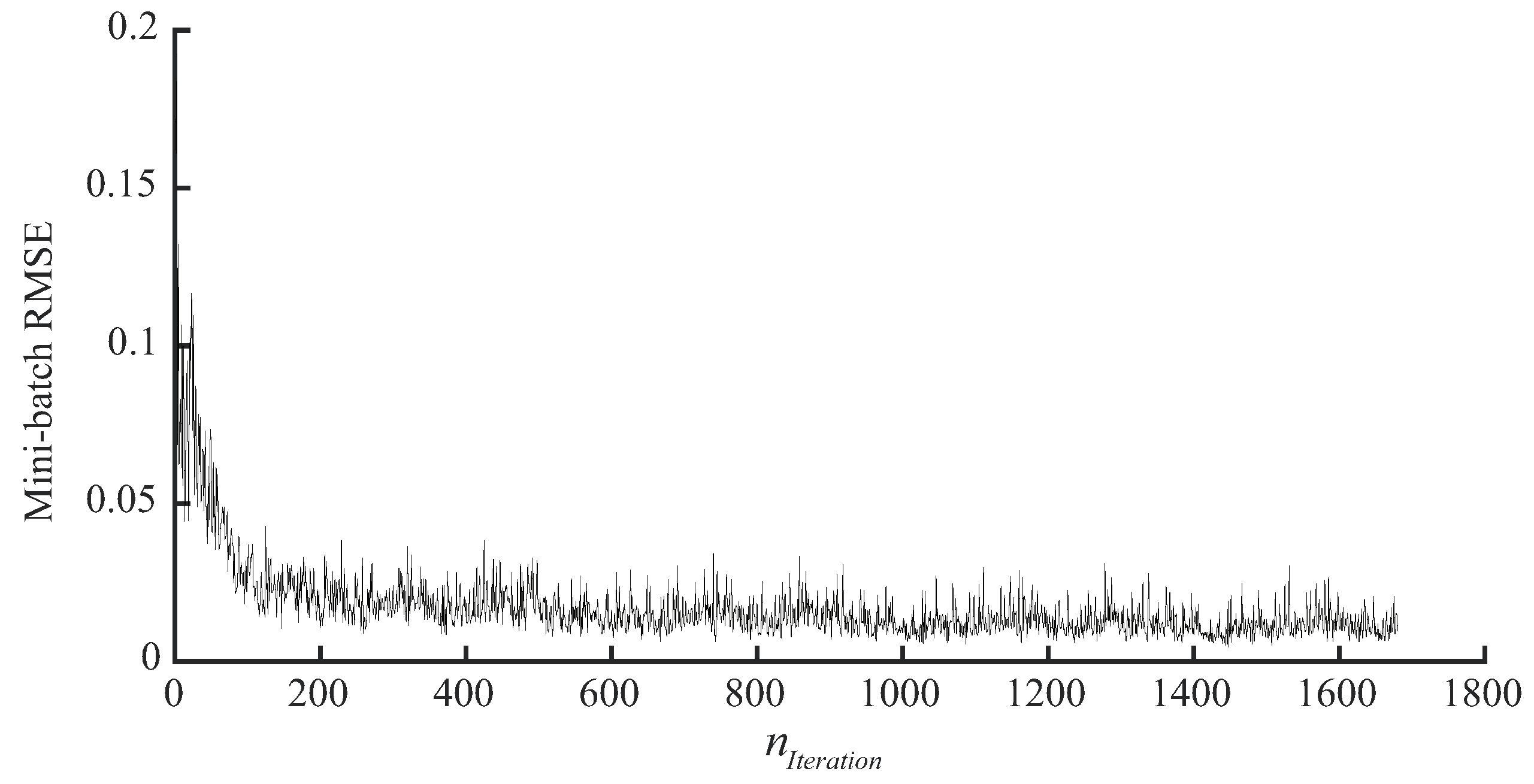
Figure 8 presents the training history with the root mean squared error (RMSE) of the minibatch, where the RMSE was calculated by the following formula:

$$RMSE=\sqrt{MSE}=\sqrt{{\displaystyle \sum _{j=1}^{s_{batch}}}\frac{{\left({\displaystyle \sum _{i=1}^{n_{coeff}}}\frac{{(y_i-x_i)}^2}{n_{coeff}}\right)}_j}{s_{batch}}}$$

(2)

where $n_{Iteration}$ represents the number of iterations. For better observation, only the minibatch RMSE of four epochs (1680 iterations) is given in Figure 8, showing the RMSE gradually decreasing with the number of iterations. Since airfoil images were relatively simple, the progress of extracting the feature map by filters was fast. The convergence of the CNN training progress was shallow. In the first 100 iterations, the basic features of the airfoil images were mainly extracted, and the RMSE converged faster. After that, features were only fine-tuned, and RMSE convergence speed was also reduced. More epochs do not necessarily mean a better result. Too many epochs lead to overfitting.

3.3. Discussion

In total, 840 test samples were fed to the trained prediction model to validate the prediction model; prediction time was 0.96 s. this was very short and could be ignored, so the time consumption of this method was mainly during model training. The time of one CFD evaluation was about 6 min (350 s), which was shorter than the model-training time. However, it often needs to calculate hundreds of flight states in practical application, so the CFD method consumes more time.

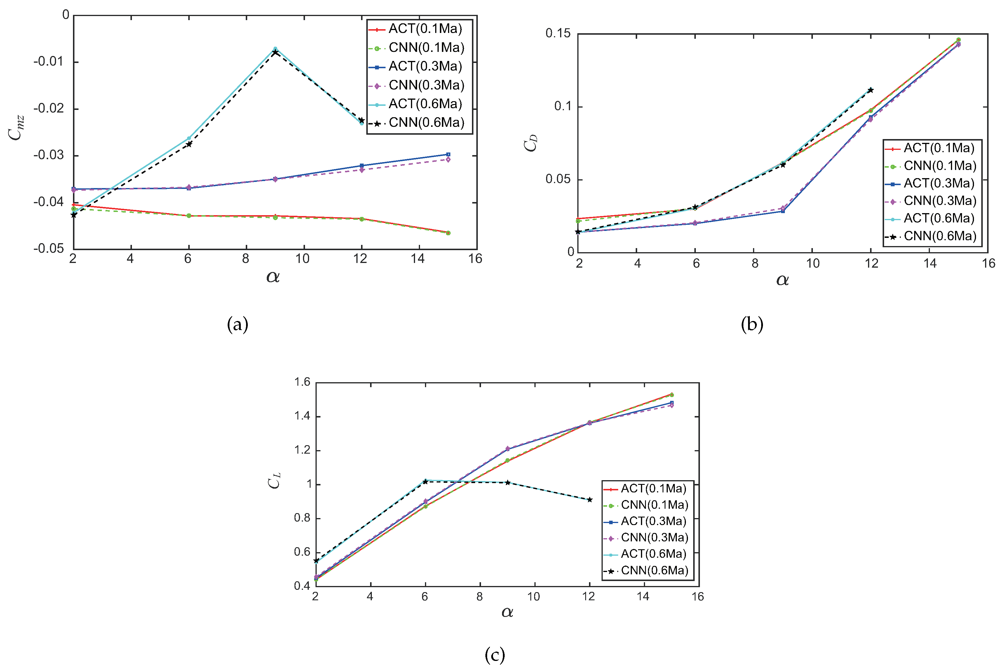
Comparisons between the actual and predicted aerodynamic coefficients of an random airfoil at different angles of attack and Mach numbers are shown in Figure 9, where $C_{mz}$, $C_D$, $C_L$ represent the pitch-moment, drag, and lift coefficients, respectively; ACT represents the actual aerodynamic coefficient; and CNN represents the predicted aerodynamic coefficient. A conclusion could be drawn, as shown in the figures, that the prediction model established in this paper could accurately predict the three aerodynamic coefficients.

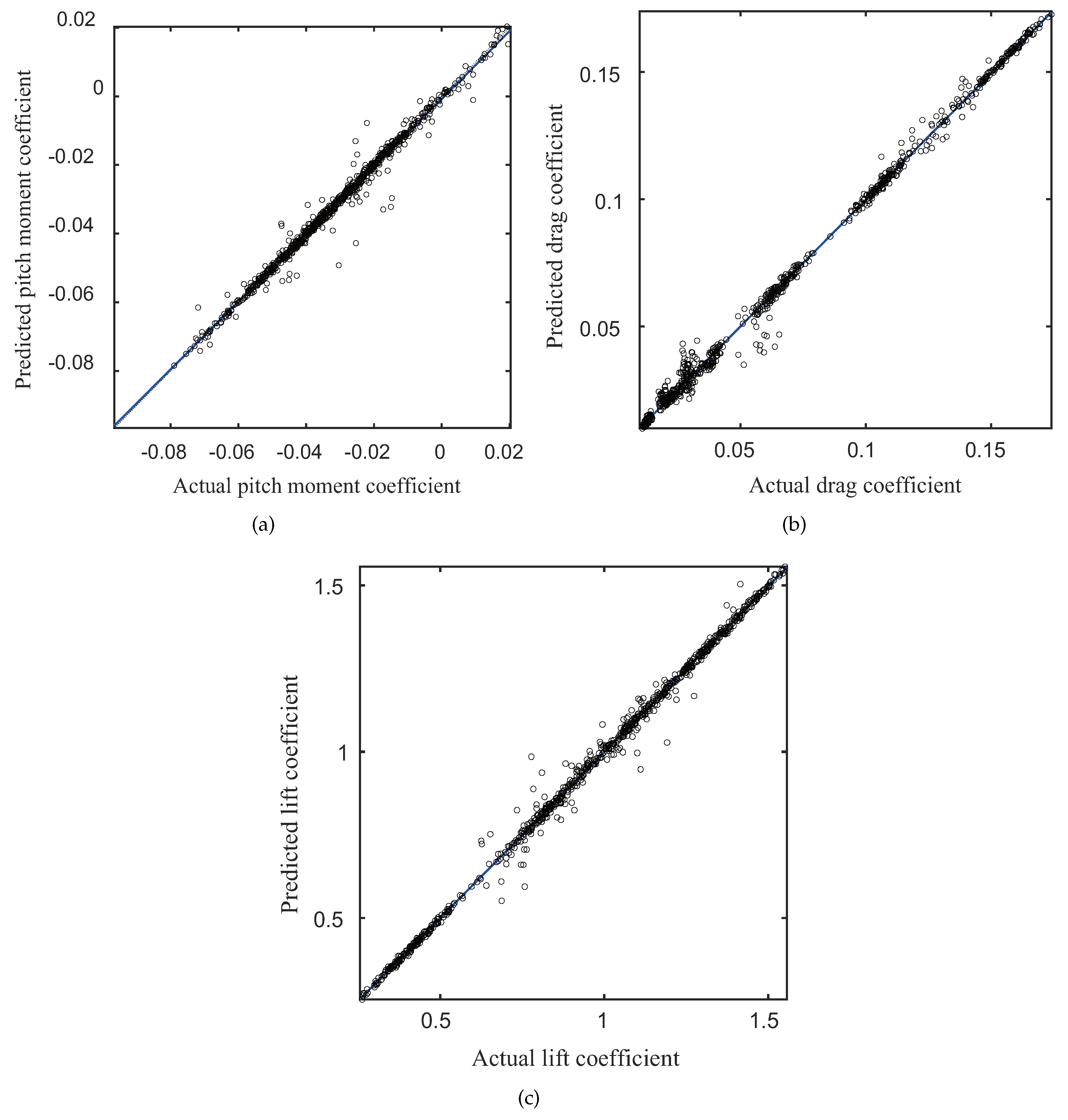
Figure 10 is the linear regressions of the actual relative to the predicted aerodynamic coefficients. The majority of points were clustered near the ${45}^{\circ }$ line, meaning that the predicted values were close to the actual values. Only a few points had a poor prediction effect. Compared with [10], prediction accuracy decreased. Previous research was to predict a single aerodynamic coefficient under fixed-flow conditions, and the prediction model was more targeted. In this paper, we established a prediction model to predict multiple aerodynamic coefficients under various flow conditions.

Table 2. Root mean squared error (RMSE) of airfoil aerodynamic coefficients.

Methods of Input Image Preparation	RMSE
	${\mathit{C}}_{\mathit{m}\mathit{z}}$	${\mathit{C}}_{\mathit{D}}$	${\mathit{C}}_{\mathit{L}}$
Method used in this paper (convolution of flow conditions and airfoil images to generate TAIs).	0.0027	0.0035	0.0273
Construct 2 $85\times 85$ constant two-dimensional input matrices using angle of attack and Mach number.	0.0030	0.0044	0.0341
Construct $85\times 85$ two-dimensional input matrix by using combination of angle of attack and Mach number. Upper part of the matrix is angles of attack, and the lower part is Mach number.	0.0052	0.0057	0.0492
Method in [10].	0.0042	0.0042	0.0296

shows the RMSE of the airfoil aerodynamic coefficients by different methods of input image preparation. The inside of the airfoil image was filled in [10]. As shown in Table 2, the RMSE of the method used in this paper was minimal. Further compared with [10], when the number of epochs was 80, it can be seen from Figure 9a of [10] that the RMSE of $C_L$ was about 0.081; after 400 epochs, it was about 0.069. In this paper, three aerodynamic coefficients were predicted at the same time. After 80 epochs, the RMSE of $C_L$ dropped to 0.0273. Compared with [10], prediction accuracy was higher.

To further demonstrate the performance of the proposed graphical method in this paper, we compared it with other two graphical methods. The CNN network was replaced with a Directed Acyclic Graph (DAG) network and MLP. The data-processing and training methods of the DAG network are similar to those of the CNN, but its structure is complex and training time is long. The MLP network could not directly process the image. The image could only be used as input to the prediction model if it were converted into a vector. Therefore, the resolution of the airfoil image could not be set too high. If the MLP network were selected as a three-layer network whose number of layers was [80, 10, 3], the resolution of the airfoil image had to be within $20\times 20$. Otherwise, an out-of-memory error would occur.

Table 3. Comparison of three graphical methods.

Prediction Network	Resolution of Airfoil Image	Training Time (min)	RMSE
			${\mathit{C}}_{\mathit{m}\mathit{z}}$	${\mathit{C}}_{\mathit{D}}$	${\mathit{C}}_{\mathit{L}}$
CNN	$85\times 85$	35	0.0027	0.0035	0.0273
DAG	$85\times 85$	35	0.0137	0.0413	0.2834
MLP	$16\times 16$	35	0.0028	0.0040	0.0332

shows the comparison of the three graphical methods. It can be seen from Table 3 that the CNN prediction model had the shortest training time and the highest prediction accuracy.

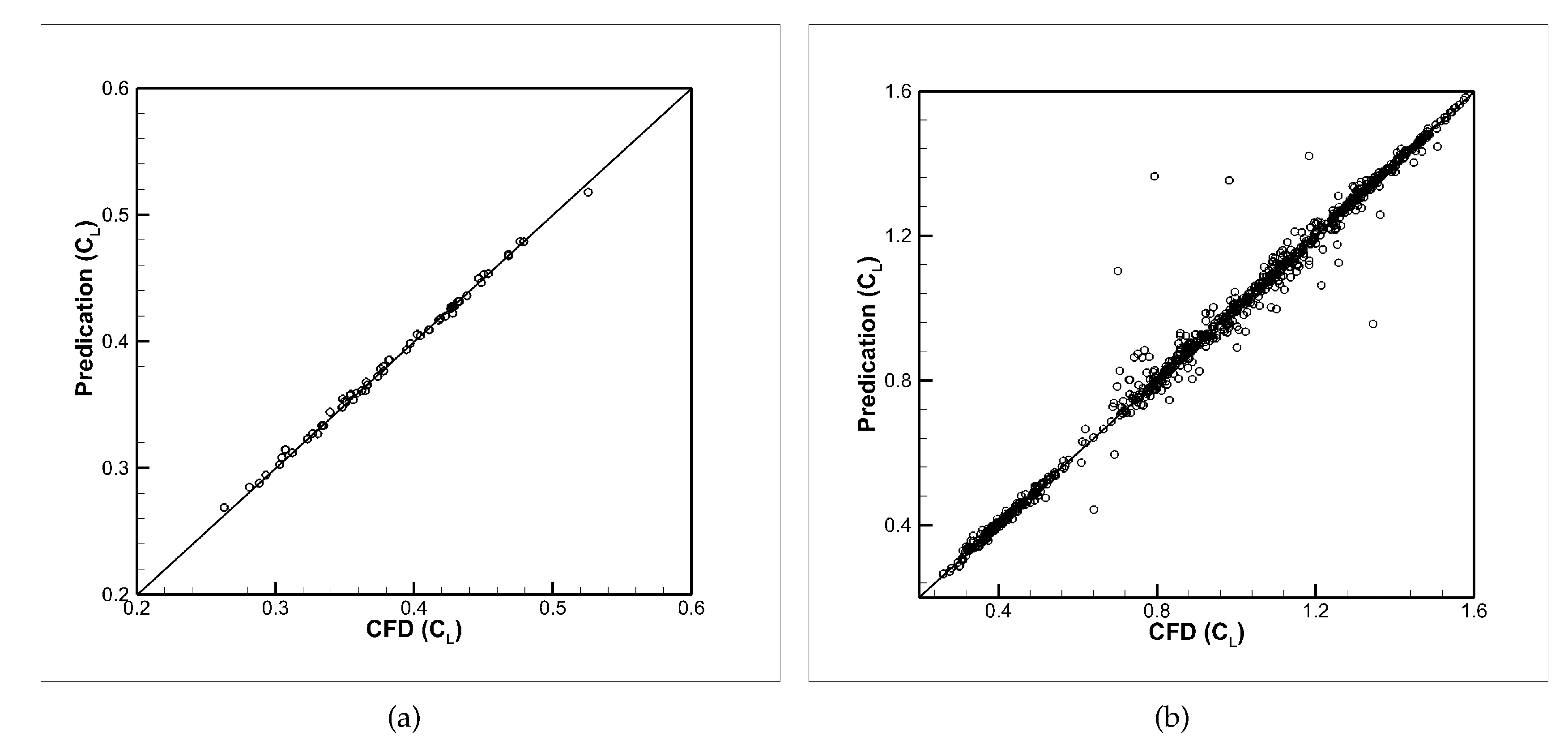
Traditionally, the kriging method is commonly used to predict the aerodynamic characteristics of airfoils, and it is a parametric method. Figure 11 and

Table 4. Results of kriging model.

Case	Training Time (s)	RMSE	Mean Relative Error	Maximum Relative Error
Case 1 (300 samples)	192	0.0029	$0.59\%$	$2.44\%$
Case 2 (4200 samples)	85,095	0.0433	1.94%	80.20%

show the predicted results of $C_L$ in two different cases with the kriging method. In Case 1, there were 300 samples selected from the 4200 samples at a fixed-flow condition: attack angle was 2 and Mach number is 0.1. In Case 2, all of the 4200 samples were used. The 80% of samples were used for training and the remaining 20% for validation in both cases. Open-source tool pyKriging was used here with a genetic optimization algorithm. The RMSE was 0.0029, mean relative error was 0.59%, and the maximal relative error was 2.44% in Case 1, which was more accurate compared with the method proposed in this paper. However, results were not so satisfactory in Case 2. Training-time consumption of the kriging model increased exponentially with the increase of samples. For example, when 100, 200, 300, 400, and 500 samples were randomly selected from 4200 samples for the kriging model, training time was 25.3, 68.5, 191.7, 389.6, and 813.5 s, respectively, and it took about 23 h (85,095 s) to train the model in Case 2. However, training-time consumption of the method proposed in this paper linearly increased with the increase of samples. Therefore, although the kriging model exactly went through the training points and could approximate the true model with fewer data [18], the method proposed in this paper was more adaptable to big data compared with the kriging method.

4. Conclusions

This paper proposed a multiple aerodynamic-coefficient prediction method of airfoils based on CNN. It convolved an airfoil image with flow conditions to generate a TAI. The TAI was combined with the original airfoil image to form a CAI, which was used as the input of the CNN to establish a prediction model. The prediction model could predict three aerodynamic coefficients of airfoils at the same time, with little time consumption and high accuracy.

Although there were a few points with substantial deviations from the optimum, most of the predicted values were close to the actual value, which proved the feasibility of the prediction method. In future research, we will continue to improve the prediction model. The latest deep-learning technology will be applied to improve prediction accuracy. At the same time, we will further explore the application prospects of deep learning in the CFD field, and predict the velocity, temperature, and pressure fields, and other parameters of the 3D model.