Article

Optimal Denoising and Feature Extraction Methods Using Modified CEEMD Combined with Duffing System and Their Applications in Fault Line Selection of Non-Solid-Earthed Network

School of Electrical and Electronic Engineering, North China Electric Power University, Baoding 071003, China
*
Authors to whom correspondence should be addressed.
Symmetry 2020, 12(4), 536; https://doi.org/10.3390/sym12040536
Submission received: 18 February 2020 / Revised: 22 March 2020 / Accepted: 23 March 2020 / Published: 3 April 2020

Abstract

:
As the non-solid-earthed network fails, the zero-sequence current of each line is highly non-stationary, and the noise component is serious. This paper proposes a fault line selection method based on modified complementary ensemble empirical mode decomposition (MCEEMD) and the Duffing system. Here, based on generalized composite multiscale permutation entropy (GCMPE) and support vector machine (SVM) for signal randomness detection, the complementary ensemble empirical mode decomposition is modified. The MCEEMD algorithm has good adaptability, and it can restrain the modal aliasing of empirical mode decomposition (EMD) at a certain level. The Duffing system is highly sensitive when the frequency of the external force signal is the same as that of the internal force signal. For automatically identifying chaotic characteristics, by using the texture features of the phase diagram, the method can quickly obtain the numerical criterion of the chaotic nature. Firstly, the zero-sequence current is decomposed into a series of intrinsic mode functions (IMF) to complete the first noise-reduction. Then an optimized smooth denoising model is established to select optimal IMF for signal reconstruction, which can complete the second noise-reduction. Finally, the reconstructed signal is put into the Duffing system. The trisection symmetry phase estimation is used to determine the relative phase of the detection signal. The faulty line in the non-solid-earthed network is selected with the diagram outputted by the Duffing system.

1. Introduction

Nowadays, the non-solid-earthed network is widely used in the distribution network. When a single phase-to-ground occurs, the line voltage of the system remains symmetrical, and it can run for 2 to 3 hours after the fault occurs. However, the phase voltage of the non-fault line could rise, which would be a severe threat to the insulation of the system. It is necessary to remove faults quickly for safety in operation. There are many difficulties in fault line selection, such as weak fault current signal and complex actual operating environment [1,2,3]. Due to the compensation effect of the arc suppression coil, the fundamental component of the zero-sequence current cannot select the fault line. However, the arc suppression coil has little influence on the high-frequency component, but the high-frequency component is non-stationary and nonlinear, and the traditional faulty line selection method would fail. It is thus necessary to conduct further research in the area.
At present, faulty line selection methods are roughly divided two ways: fault steady-state characteristic method and fault transient characteristic method [4,5]. The steady-state characteristic method mainly uses the magnitude and direction of the fundamental zero-sequence current to form the criterion. However, due to the compensation effect of the arc suppression coil, the fundamental zero-sequence current direction of the faulty line and the non-fault line may be the same, and the fundamental zero-sequence current of the faulty line may not be the maximum. The result of the steady-state characteristic method may be unreliable. The fault transient characteristic method is more reliable because the transient characteristics are abundant, and it is not affected by the compensation of the arc suppression coil. Previous studies [6,7] used wavelet transform to decompose signals and extract fault features for faulty line selection. However, the wavelet basis function needs to be accurately selected, and the frequency band selected by wavelet transform under intense noise may not be valid. Zhang, Liu, and Piao [8] used a phase-locked loop to extract the fifth harmonic zero-sequence current, and the faulty line was selected by the fifth harmonic zero-sequence current characteristics. However, if the component of other harmonic signals is significant, it will affect the accuracy of faulty line selection. Zhang and co-workers [9] used empirical mode decomposition (EMD) to analyze transient characteristics. However, when there is intensive noise in the signal, the EMD algorithm would have the problem of mode confusion and cause the failure of faulty line selection. Kang and colleagues [10] used the matrix pencil method to analyze the characteristic frequency band of transient zero-sequence current, and the faulty line was selected according to the frequency component. However, this method did not take account of the effect of noise. Li and co-workers [11] used variational mode decomposition (VMD) to deal with nonlinear signals. VMD does not need to use the recursive decomposition process. It alleviates some deficiencies in EMD and has been applied in the field of signal processing. However, it is limited by the selection of the number of decomposition layers. Ensemble empirical mode decomposition (EEMD) improves the mode confusion problems of the EMD algorithm by adding different white noises to the original signal repeatedly [12,13,14,15]. However, the added white noises can cause reconstruction error. Complementary ensemble empirical mode decomposition (CEEMD) can decrease the reconstruction error of the EEMD by adding opposite white noises to the target signal [16,17,18]. However, if the amplitude of the added white noise and the number of iterations are not appropriate, the result would be many pseudorandom components. Some useful characteristics will be lost when the high-frequency signal is filtered, which will affect the denoising effect. Complete ensemble empirical mode decomposition with adaptive noise (CEEMDAN) has been applied for denoising of the nonlinear signals [19,20,21]. However, CEEMDAN still has noise existing in the result of intrinsic mode functions, and some intrinsic mode functions could exist in hysteretic intrinsic mode functions.
This paper extracts the transient characteristics of the zero-sequence current accurately based on modified complementary ensemble empirical mode decomposition (MCEEMD) and the Duffing system. The pseudorandom components of CEEMD’s intrinsic mode functions (IMF) are eliminated according to generalized composite multiscale permutation entropy (GCMPE) and support vector machine (SVM). The EMD decomposes the remaining intrinsic mode functions. The results are arranged in the order from high frequency to low frequency, namely, the MCEEMD algorithm. MCEEMD is a process of smoothing the signal, which can adaptively decompose the signal into a series of intrinsic mode functions according to the local scale characteristics of the signal. MCEEMD algorithm can suppress the mode confusion of the EMD algorithm and has better completeness and orthogonality than the CEEMD algorithm. The optimal intrinsic mode functions are selected to ensure that the filtered signal has preferable similarity and smoothness by an optimal smooth denoising model. The filtered signal can reduce the noise content and contain the useful components of the original signal. Wang and colleagues [22] proposed that the Duffing system is highly sensitive to a weak signal. In this paper, a new method of identifying chaotic characteristics based on texture features of the phase diagram is proposed. It has such advantages as visibility, a simple algorithm, and a small computational amount. Every line’s filtered signal is input into the Duffing system as a characteristic value, and the faulty line is selected by the change of the phase diagram of the system.

2. Generalized Composite Multiscale Permutation Entropy

2.1. Permutation Entropy

Permutation entropy (PE) can detect the randomness and dynamic behavior of a time series. It has a strong anti-interference ability and is suitable for dealing with nonlinear data [23,24]. Given a time series {x(i) i = 1, 2, …, N} with length N, the time series is reconstructed as follows:
X ( 1 ) = { x ( 1 ) , x ( 1 + τ ) , , x ( 1 + ( m 1 ) τ ) } X ( i ) = { x ( i ) , x ( i + τ ) , , x ( i + ( m 1 ) τ ) } X ( N ( m 1 ) τ ) = { x ( N ( m 1 ) τ ) , x ( N ( m 2 ) τ ) , , x ( N ) }
where m is the embedded dimension, and τ is a time delay. The m elements in X(i) are rearranged in ascending order as
x ( i + ( j 1 1 ) τ x ( j + ( j 2 1 ) τ )   x ( i + ( i + j m 1 ) τ ) .
For x ( i + ( j i 1 1 ) τ ) = x ( i + ( j i 2 1 ) τ ) , the permutation is ordered as x ( i + ( j i 1 1 ) τ ) x ( i + ( j i 2 1 ) τ ) for j i 1 j i 2 . Each vector X(i) gets a set of symbol sequences as
S ( g ) = [ j 1 , j 2 , , j m ] ,
where g = 1 ~ k ,   k m ! . Due to m different symbols [ j 1 , j 2 , , j m ] , there are m! different symbol arrangements. S(g) is just one of m! symbol arrangements. The frequency of each symbol arrangement is defined as Pg (g=1, 2, …, k). The PE can be calculated according to the Shannon entropy as
H p ( m ) = g = 1 k P g ln P g ,
when P g = 1 / m ! , the maximal value of Hp(m) is ln(m!). The standardized PE is calculated as
H p = H p ( m ) ln ( m ! ) ,
where 0 H p 1 . When the value of Hp is larger, the time series is rather more complex. On the contrary, the time series is rather more regular.

2.2. Multiscale Permutation Entropy

Since PE is only a single-scale analysis of time series, it has some limitations. In order to solve this deficiency, multiscale permutation entropy (MPE) is proposed. The most crucial step of this algorithm is to make the time series coarse-grained [25]. Given a time series {x(i) i = 1, 2, …, N} with length N, the coarse granulation’s process is calculated as
y j ( s ) = 1 s i = ( j 1 ) s + 1 j s x ( i ) , 1 j N s ,
where s is the scale factor, and y j ( s ) is a new time series at a scale factor, namely, coarse-grained series. The PE of each coarse-grained time series can be calculated. MPE is made of these PE values:
MPE ( X , s , m , τ ) = PE ( y ( s ) , m , τ ) .
Although MPE can overcome the single time scale problem of PE, the method still has some deficiencies. The process of coarse granulation is unique, and some vital information would inevitably be lost [26,27,28]. The results of MPE may show an unstable trend.

2.3. Generalized Composite Multiscale Permutation Entropy

Zheng [29] proposed the GCMPE algorithm solving the deficiencies of MPE. The algorithm is listed as follows: Firstly, the PE values of all coarse-grained sequences in the same scale factor are calculated, and all entropy values are averaged. Secondly, the first moment (average) can be extended to the second moment (variance), namely the GCMPE method. The generalized coarse-grained sequence can be expressed as
y k , j ( s ) = 1 s i = ( j 1 ) s + k j s + k 1 ( x i x i ¯ ) 2 1 j | N s | ,   1 k s ,
where x i ¯ = 1 s k = 0 s 1 x i + k . For scale factor s, we calculate s generalized coarse-grained sequences’ PE values. Then, GCMPE ( X ,   s ,   m ,   τ ) can be expressed as
GCMPE ( X ,   s ,   m ,   τ ) = 1 s k = 1 s PE ( y k ( s ) ,   m ,   τ ) .
The coarse granulation’s processes of MPE and GCMPE with s = 3 are shown in Figure 1. The MPE can only decompose one sequence, so some crucial information would inevitably be left out. GCMPE can decompose three sequences. It can synthesize the info of multiple coarse-grained sequences at the same scale and extend the first moment (average) to the second moment (variance). Theoretically, GCMPE is better than MPE [29].

2.4. Parameter Selection and Comparative Analysis

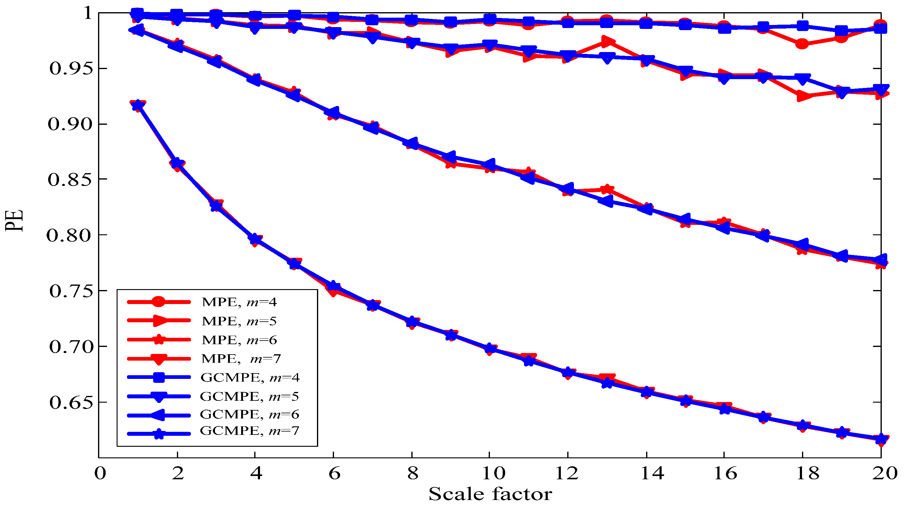
To study the influence of the embedding dimension on the calculation results, MPE and GCMPE were used to analyze the Gaussian white noise under the conditions of m = 4, 5, 6, 7. The result is shown in Figure 2. In Figure 2, it can be seen that when the embedded dimension m increased, the fluctuation and deviation of MPE increased. However, as the embedded dimension m increased, the changing trend of GCMPE is relatively smooth, and the swing is small. The comparison results show the superiority of GCMPE. As the embedded dimension m is small, the value of GCMPE does not change obviously, which cannot reflect the advantages of multi-scale analysis. On the other hand, as the value of m is large, the reconstructed time series will be homogenized, and GCMPE cannot reflect the subtle changes of the sequence [29]. Therefore, the embedded dimension m is set to 6 in this paper. If the maximal scale factor smax is >10, the GCMPE can reflect the crucial information of the signal. The time delay τ has little effect on GCMPE. Consequently, the maximal scale factor smax is set to 16, and the time delay τ is set to 1.

2.5. Signal Randomness Detection

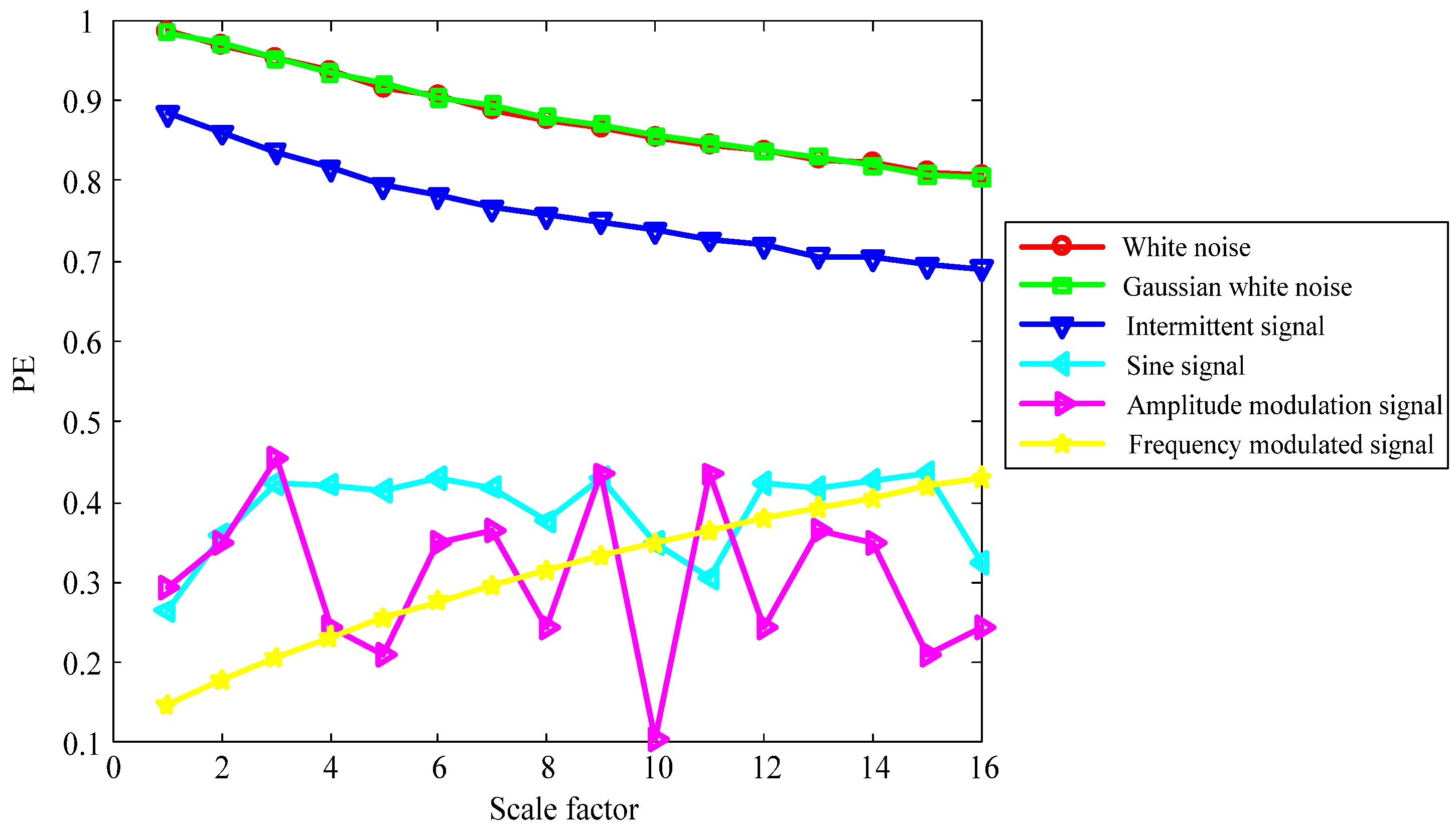
The randomness tests of white noise, Gaussian white noise, intermittent signal, sine signal, amplitude modulation signal, and frequency modulated signal are analyzed by GCMPE. The result is shown in Figure 3. From Figure 3, it is easy to know that the GCMPE values of white noise, Gaussian white noise, and intermittent signals are larger, indicating that these signals are more random. In contrast, the GCMPE values of other signals are smaller, meaning that these signals are more regular. The obtained results are consistent with the actual situation. Namely, the GCMPE value of the random signal is greater than that of the regular signal.
The SVM algorithm, which is suitable for small sample classification, is introduced to realize the intelligent detection of abnormal signals. We collected 239 signals, including 70 regular signals and 169 random signals. After obtaining their GCMPE values, the GCMPE values of 120 signals were randomly selected as the training samples of SVM, and the rest of the GCMPE values of the signals were used as the test samples. The penalty parameter c = 0.25 and kernel function parameter g = 0.0625 of SVM were calculated by K-fold cross-validation [30]. The output result was 1, which represents the regular signal; the output result was 2, which represents the abnormal signal. The recognition rates of signal types are 100%.
Through the simulation experiment, it can be seen that GCMPE-SVM can be used to detect abnormal signals.

3. MCEEMD Algorithm

3.1. The Steps of MCEEMD

After the abnormal signal is decomposed, it is not necessary to use EMD to decompose the added noises completely. Given the advantages of the GCMPE-SVM, MCEEMD can be designed. Firstly, the original signal is decomposed by CEEMD. Secondly, the IMF decomposed by CEEMD is detected by GCMPE-SVM, and the abnormal signal is eliminated from the original signal. Finally, the residual signal is decomposed by EMD, namely MCEEMD algorithm.
The detailed steps of the modified method are as follows:
Step 1: Add K pairs of opposite white noises to the original signal I(t) as follows:
{ I i + ( t ) = I ( t ) + a i n i ( t ) I i ( t ) = I ( t ) a i n i ( t ) ,
where ni(t) (i = 1, 2, …, K) is white noise, and its mean value is 0; ai is noise amplitude, and its value is 0.2 times the standard deviation of the original signal I(t).
Step 2: EMD decomposes each signal in the set. Each signal can get a series of intrinsic mode function components. The jth intrinsic mode function of the ith signal is IMFij.
Step 3: The corresponding intrinsic mode functions are averaged to eliminate white noise as much as possible:
IMF j = 1 2 K i = 1 2 K IMF i j ,
where IMFj is the jth intrinsic mode function, which is obtained by CEEMD.
Step 4: The GCMPE of each intrinsic mode function of CEEMD decomposition is analyzed by using SVM. When the output value is 2, the intrinsic mode function is considered to be an abnormal signal and is removed from the original signal. Supposing p modes are abnormal components. Then the residue signal R(t) is defined as
R ( t ) = I ( t ) i = 1 p IMF i .
Step 5: The R(t) is decomposed by EMD to obtain the MCEEMD’s IMF. The results are arranged in the order from high frequency to low frequency.

3.2. Analysis of the Simulation Signal Using EMD, CEEMD, and MCEEMD

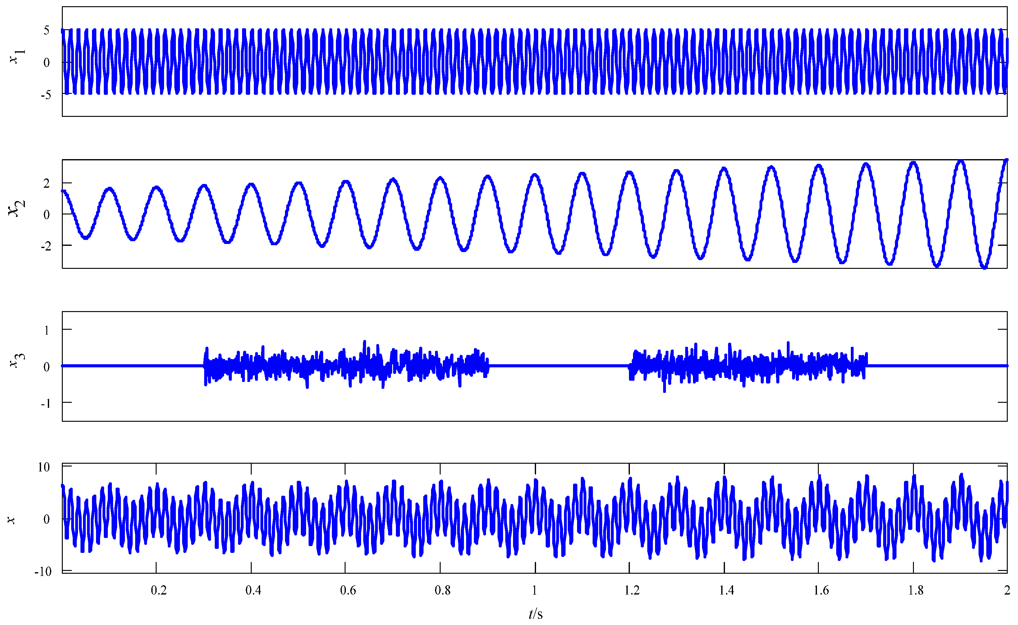
In order to demonstrate the advantages of the MCEEMD, the simulation experiments are carried out in this section. The artificial signals are given by Equation (13), where x is composed by x1, x2, and x3, and the sampling frequency is 1000 Hz. The original signals are shown in Figure 4.
{ x 1 = 5 sin ( 120 π t + π / 4 ) x 2 = ( t + 1.5 ) sin ( 20 π + π / 2 ) x 3 = [ zeros ( 1 , 300 ) , 0.2 · randn ( 1 , 600 ) , zeros ( 1 , 300 ) , 0.2 · randn ( 1 , 500 ) , zeros ( 1 , 300 ) ] x = x 1 + x 2 + x 3
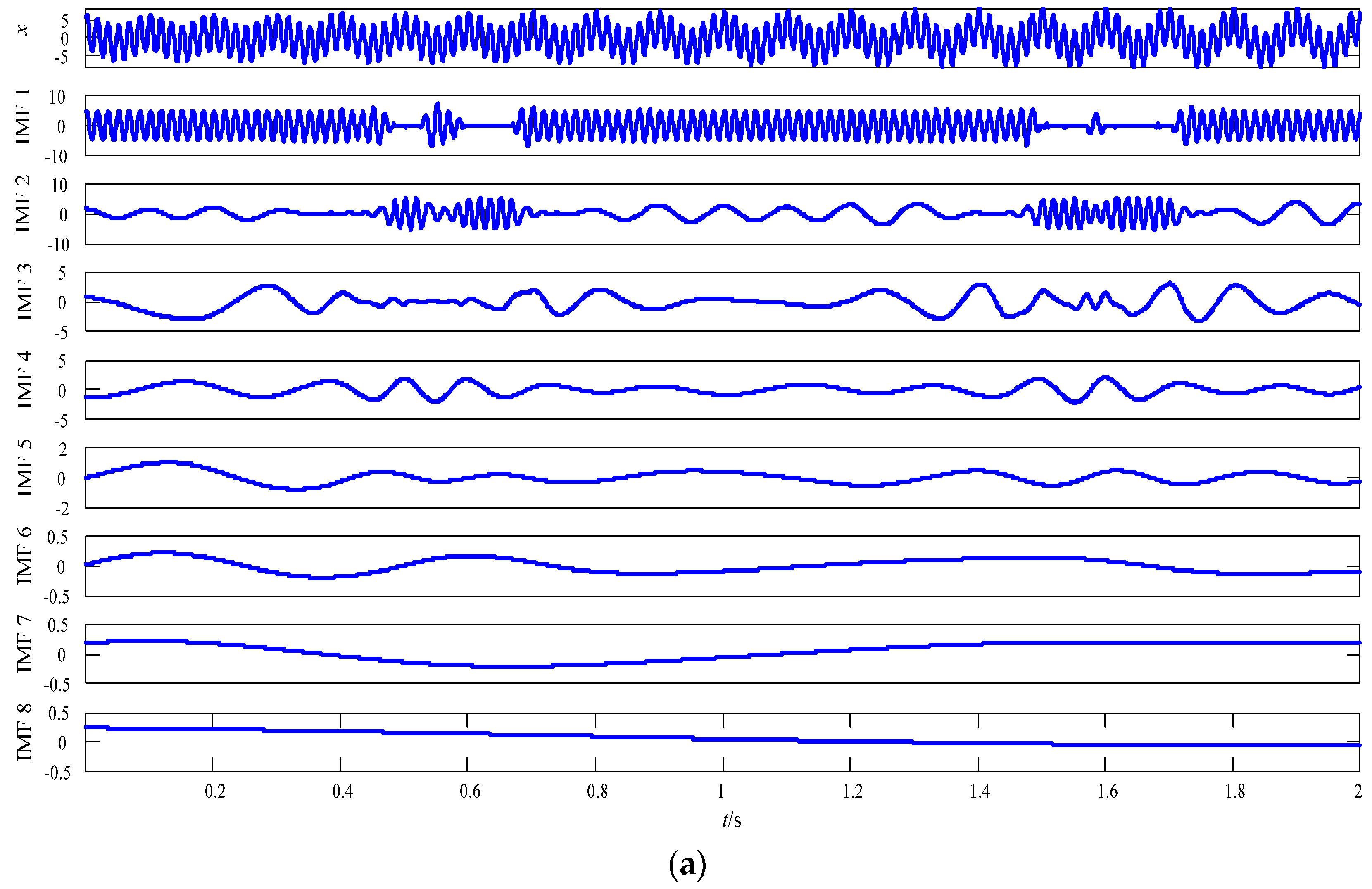
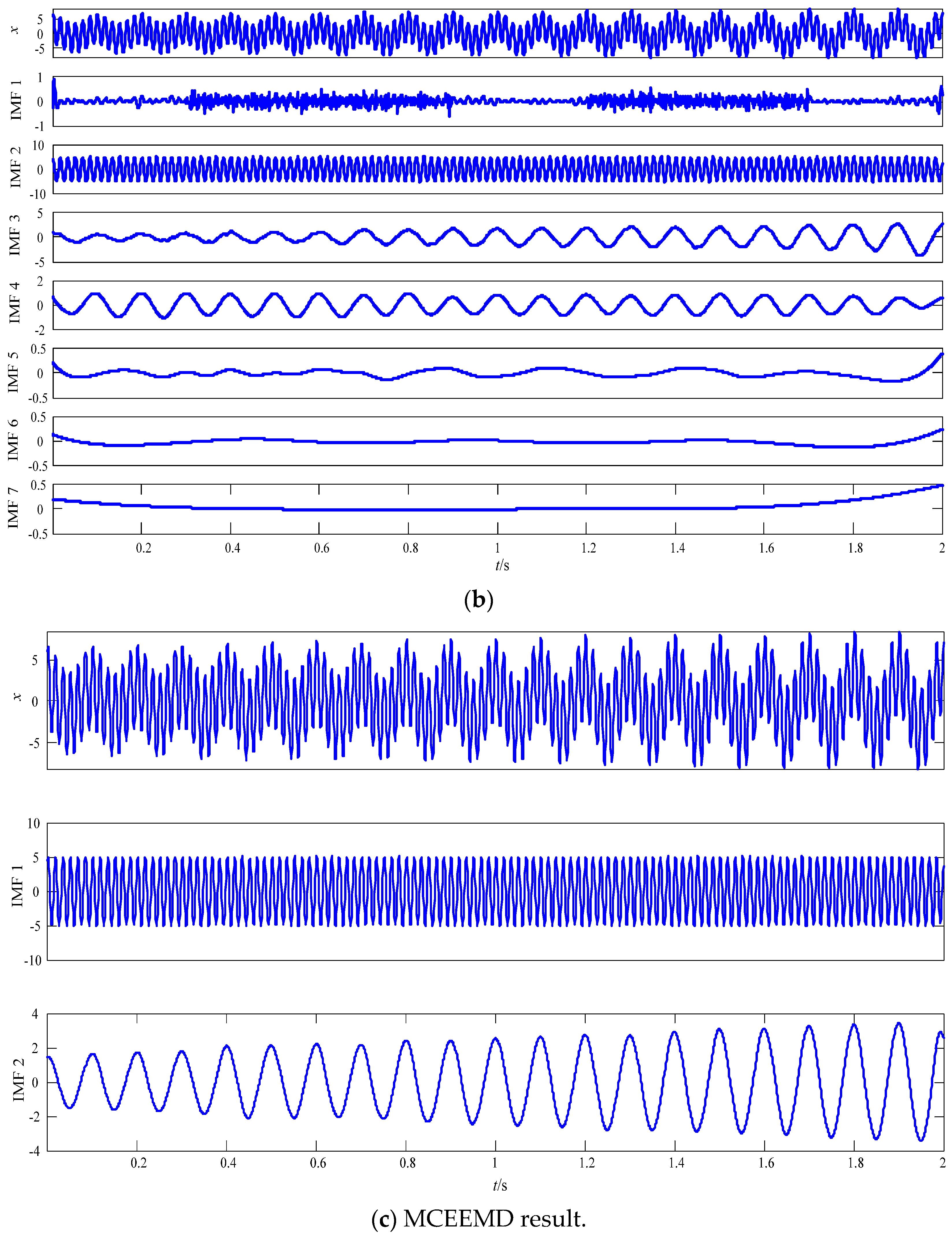
EMD, CEEMD, and MCEEMD are used to decompose x. The decomposition results are shown in Figure 5.
In Figure 5a, it is evident that the EMD algorithm has the problem of mode confusion. It is also seen in Figure 5b that the CEEMD algorithm produces false components. As can be seen in Figure 5c, the MCEEMD has no spurious components, and it removes the noise components. The correlation coefficient [1,16] can be used to analyze the degree of linear association between variables. The correlation coefficient is close to 1, indicating a higher correlation between the two variables. In addition, Table 1, Table 2 and Table 3 show the correlation coefficients of the three decomposition methods. As can be seen in Table 1, the EMD algorithm cannot extract x2 effectively. In Table 2, it is evident that CEEMD’s IMF3-IMF4 and x2 have a higher correlation. Here, the CEEMD decomposition encounters the mode confusion at a certain level. In Table 3, MCEEMD can effectively extract x1 and x2, and it restrains mode confusion. The results show that the method proposed in this paper can effectively extract the useful components of the original signal, and it suppress mode mixing at a certain level.
The index of orthogonality (Ort) can be used as a valid index to evaluate the inhibition of the end effect [31]. The smaller the Ort, the better the decomposition effect. Ort is shown in Table 4 where the Ort of MCEEMD is 5.8701 × 10 5 , and the value is almost close to 0. The results show that the Ort of MCEEMD is better than that of the other two algorithms.
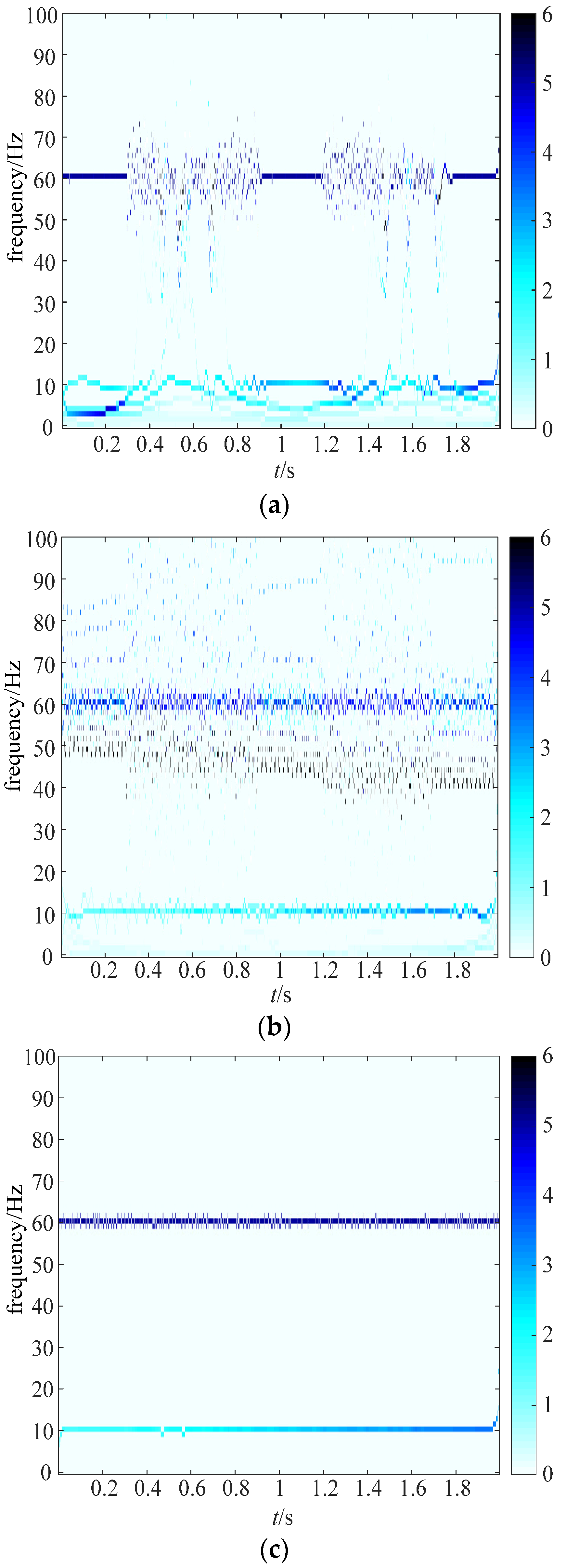
Hilbert–Huang transformation gains its popularity to analyze signals in time and frequency domains [32]. Figure 6 provides the Hilbert–Huang spectrums for three decomposition methods. As can be seen in Figure 6a, the result of EMD has a visible phenomenon of frequency mixing at 10 Hz, and the instantaneous frequency has an apparent fluctuation. Figure 6b shows the decomposition result of CEEMD has many pseudo components between 50 Hz to 90 Hz, and its instantaneous frequency is also unstable. However, the result in Figure 6c shows that MCEEMD can extract the effective components of the original signal, and there are no pseudo components in the Hilbert–Huang spectrum, and its instantaneous frequency is stable. To summarize, it is evident that the proposed algorithm has better decomposition results and overcomes mode mixing.

4. Optimal Smooth Denoising Model

4.1. Optimal Smooth Denoising

The optimal smooth denoising model is composed of the MCEEMD and the objective function. The objective function takes into account the similarity and smoothness of different filtering algorithms. MCEEMD decomposes the original signal I(t), and the signal reconstruction SR(t) can be obtained as
S R k ( t ) = i = 1 k IMF i ,
where SRk(t) represents the kth signal reconstruction, and i is the number of the IMF.
The standard deviation of the difference value between the signal reconstruction SR(t) and the original signal I(t) is taken as the similarity standard [33], like
{ X ( t ) = I ( t ) S R ( t ) Amse = std ( X ( t ) ) = i = 1 N ( X ( i ) X ¯ ) 2 N 1 ,
where N is the number of sample points, and Amse represents the similarity standard. The smaller Amse, the closer the reconstructed signal is to the original signal.
If the function f(x) on the interval (a, b) is assumed to have a continuous first-order derivative, its figure is a curve with tangents everywhere, and the tangents rotate continuously with the movement of the tangent point. The curve is defined as a smooth curve. In particular, it is obtained that a necessary and sufficient condition for function derivable at a certain point is that the left and right derivatives of the point coexistent and are equal. Suppose the point x1 lies on the curve f(x). The left curvature and the right curvature at point x1 are as follows:
{ K = | f ( x 1 ) | ( 1 + ( f ( x 1 ) ) 2 ) 3 / 2 K + = | f + ( x 1 ) | ( 1 + ( f + ( x 1 ) ) 2 ) 3 / 2 ,
where K and K + are the left curvature and the right curvature, respectively. If f(x) is smooth and differentiable at x = x1, the left curvature and the right curvature at x1 are equal as follows:
K = K +   | f ( x 1 ) | = | f + ( x 1 ) | .
f ( x 1 ) and f + ( x 1 ) are expanded to the difference forms as follows:
{ f ( x 1 ) f ( x 1 2 h ) 2 f ( x 1 h ) + f ( x 1 ) h 2 f + ( x 1 ) f ( x 1 + 2 h ) 2 f ( x 1 + h ) + f ( x 1 ) h 2   ,
where h represents the sampling step. It is evident, therefore, that if f(x) is smooth and differentiable at x = x1, it means f ( x 1 ) = f + ( x 1 ) . The smoothness of the signal reconstruction at x = x1 can be defined as
S N | x = x 1 = f ( x 1 + 2 h ) f ( x 1 2 h ) 2 [ f ( x 1 + h ) f ( x 1 h ) ] ,
where SN is the smoothness index of the signal reconstruction at x = x1. The standard deviation of SN values of all points is taken as the smoothness index of the whole signal reconstruction as
Asmse = std ( S N ) ,
where Asmse represents the smoothness standard. The smaller Asmse, the smoother the signal reconstruction SR(t). Thus, the objective function Aminf can be defined as
Aminf = μ Amse + ( 1 μ ) Asmse ,
where μ is the weight factor, and 0 μ 1 . The factor μ can be valued by balancing the requirements of the similarity and smoothness. It is set to 0.6 in this paper. As Aminf gets the minimum, the objective function can achieve an optimal solution, and then match the optimal solution with the filtering algorithm, namely, the optimal smooth denoising model.

4.2. Optimal Smooth Denoising Experiment of Simulation Signal

In order to validate the effectiveness of the optimal smooth denoising model, it is utilized to analyze simulation signals. The simulation signals are given as follows:
{ x 1 = sin ( 25 π t + cos ( 50 π t ) ) x = x 1 + n o i s e ,
where x1 represents the clear signal, and x is the noisy signal. The x1 is shown in Figure 7a; x is composed of x1 and Gaussian white noise as shown in Figure 7b.
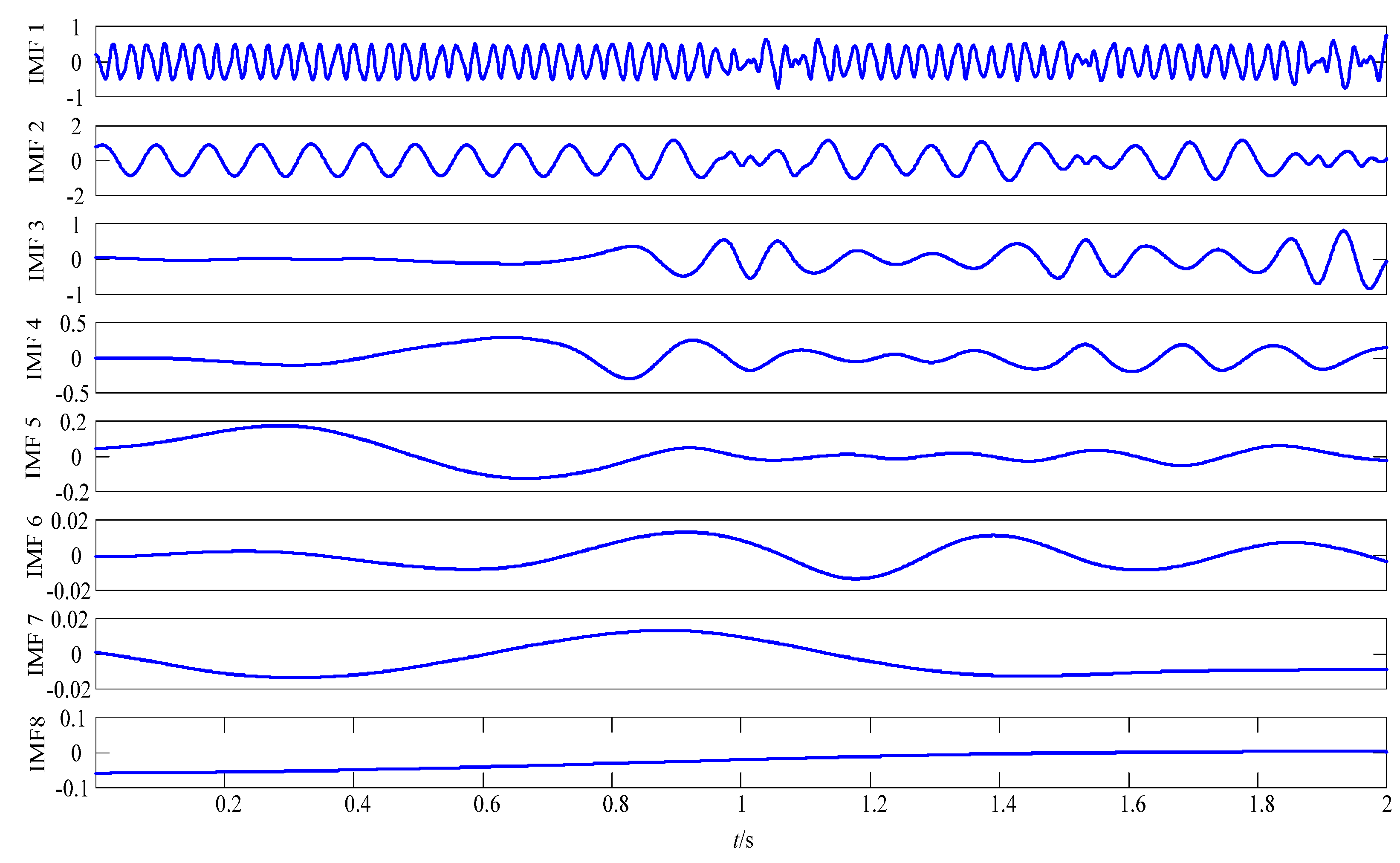
The noisy signal x is decomposed by the MCEEMD. The results are shown in Figure 8. From Figure 8 it is easy to know that the MCEEMD decomposition results can get eight components.
Different filtering algorithms are established based on the eight components obtained by the MCEEMD decomposition results as follows:
{ S R 1 = I M F 1 S R 2 = i = 1 2 IMF i S R 3 = i = 1 3 IMF i S R 8 = i = 1 8 IMF i   ,
The similarity standard Amse, the smoothness standard Asmse, and the objective function Aminf of each filtering algorithm are listed in Table 5. As shown in Table 5, based on these results, the filtering algorithm SR8 is thought to be optimal when the similarity standard Amse and the smoothness standard Asmse are comprehensively considered.
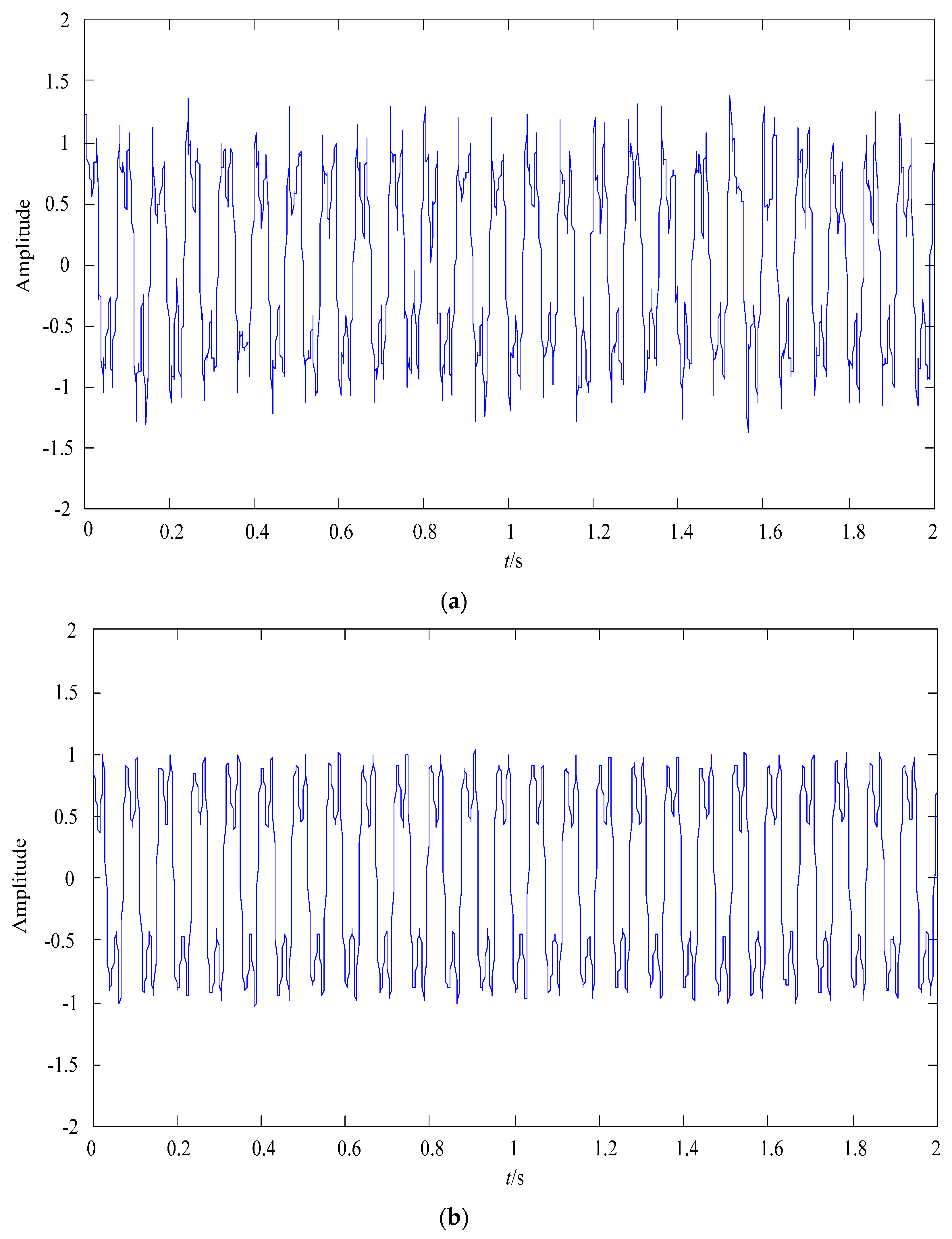
In order to prove the excellent performance of the optimal smooth denoising model, the filtering algorithm SR8 is compared with the wavelet threshold denoising. The results are shown in Figure 9.
As shown in Figure 9a, it can be seen that the waveform still contains noises. The signal-to-noise ratio of the wavelet threshold denoising is 10.9047 dB. The wavelet threshold denoising also confronts the problems of how to choose the wavelet base and wavelet decomposition level. For the optimal smooth denoising model, its signal-to-noise ratio is 11.0150 dB, and the similarity coefficient between its result and the clear signal x1 is 0.9971. To summarize, the proposed denoising method not only can retain the accurate information of the original signal but also can reduce the noise and smooth the original signal.

5. Measuring Principle of Duffing System

5.1. Duffing System Model

The Duffing system is widely used in weak signal detection [34,35,36]. When it is in the critical state, a minimal change of its parameters can cause the change of the system state. For the fifth harmonic, the amplitude of the fault line is large relatively, and the phase of the fault line is opposite to that of the non-fault lines. The fifth harmonic components of the fault line and the non-fault line can change the Duffing system into different state trajectories. The normal form of the Duffing equation can be defined as
x + k x x + x 3 = r cos ( t ) ,
where k represents the damping ratio, and rcos(t) denotes the internal driving force. x + x 3 is a non-linear restoring force. The equivalent form of the Duffing equation can be expressed as
{ x = y y = x x 3 k y + r cos ( t ) .
The damping ratio k is fixable, and it is set to 0.5 in this paper. As the internal driving force amplitude r varies from small to big, the Duffing system can have different motion states. If r = 0, the system will have three singular points; (0, 0) is the saddle point and (±1, 0) is the center point. When r exceeds a certain threshold rc, the trajectory of the system turns into a chaotic state. If r continues increasing over a certain threshold rd, the trajectory of the system changes from the chaotic state to the large-scale periodic motion state. The state at rd is used to detect the signal. rd can be previously determined by the computer simulation experiment [37]. Based on the experiments, we chose rd = 0.8253. For detecting the high-frequency signal, we must do time scale transformation. Defining t = ω τ , we obtain
1 ω 2 d 2 x d τ 2 + k ω d x d τ x + x 3 = r d cos ( ω τ ) + a cos ( ω τ + φ ) ,
where a cos ( ω τ + φ ) is the input signal. The total driving force can be expressed as
F ( t ) = r d cos ( ω τ ) + a cos ( ω τ + φ ) = r cos ( ω t + θ ) ,
where
{ r = r d 2 + 2 r d a cos φ + a 2 θ = arctg a sin φ r d + a cos φ .
Since a<<rd, θ is very small, and its impact on the system can be negligible. If π arccos ( a / 2 r d ) φ π + arccos ( a / 2 r d ) , r r d , the trajectory of the Duffing system is still in a chaotic state. If θ is not in this range, it makes the transition from the chaotic state to the large-scale periodic motion state. Making use of the characteristic of the Duffing system can select the fault line in the non-solid-earthed network. In this paper, the angular frequency of the internal driving force is set as 500π rad/s, and the calculated step size is set as 5 × 10⁻⁶. For ignoring the effect of θ , the input signal shall be multiplied by a detection factor. We chose different detection factors for experiments, and 0.01 had the best effect.

5.2. Trisection Symmetry Phase Estimation

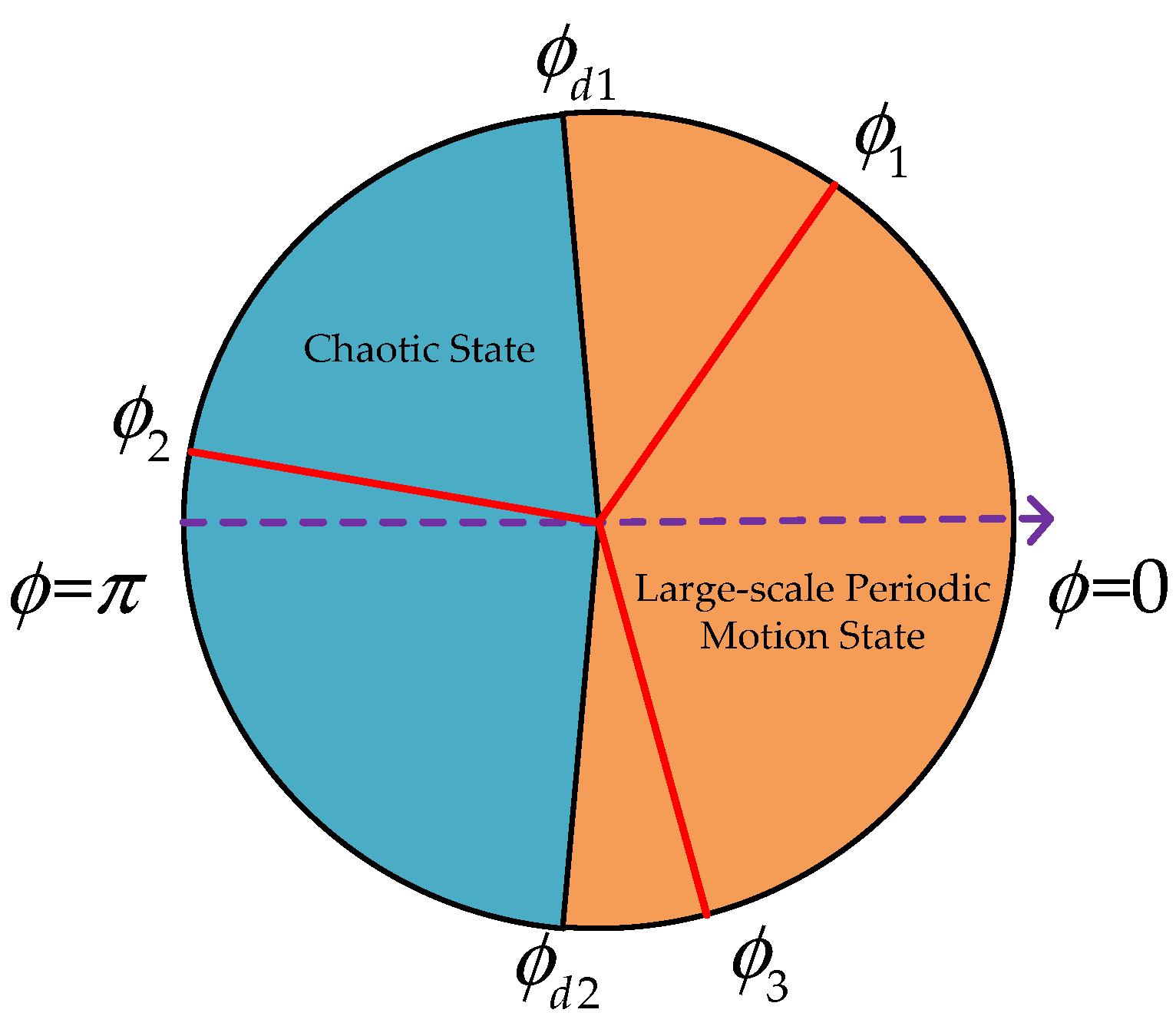
Trisection symmetry phase estimation (TSPE) can determine the phase of the input signal relative to the internal driving force [38]. The detection process of TSPE is shown in Figure 10. In Figure 10, ϕ d 1 and ϕ d 2 are the critical phase sites. Dividing the 2π area into three equal parts, we shift the phase of the input signal by 0, 2π/3, and 4π/3, respectively. The phase-shifted signals are input into the Duffing system in turn. There must be a phase’s motion state, which is different from the other two phases’ motion states. From Figure 10, it can be seen that ϕ 2 is in the chaotic state, however, ϕ 1 and ϕ 3 are in the large-scale periodic motion states. Hence, it is concluded that critical sites are located in ( ϕ 1 ,   ϕ 2 ) and ( ϕ 2 ,   ϕ 3 ) . The dichotomy is used to reduce the search area of the critical phase within ( ϕ 1 ,   ϕ 2 ) and ( ϕ 2 ,   ϕ 3 ) . The process continues until the critical phase is searched.
A line’s zero-sequence current, which is denoised by the optimal smooth denoising model of MCEEMD, is the selected signal. TSPE determines the critical phase. Moving all line signals synchronously according to the critical phase, we input them into the Duffing system. The fault line and the non-fault line can make the Duffing system in different state trajectories.

5.3. A Method of Distinguishing Chaotic Characteristics

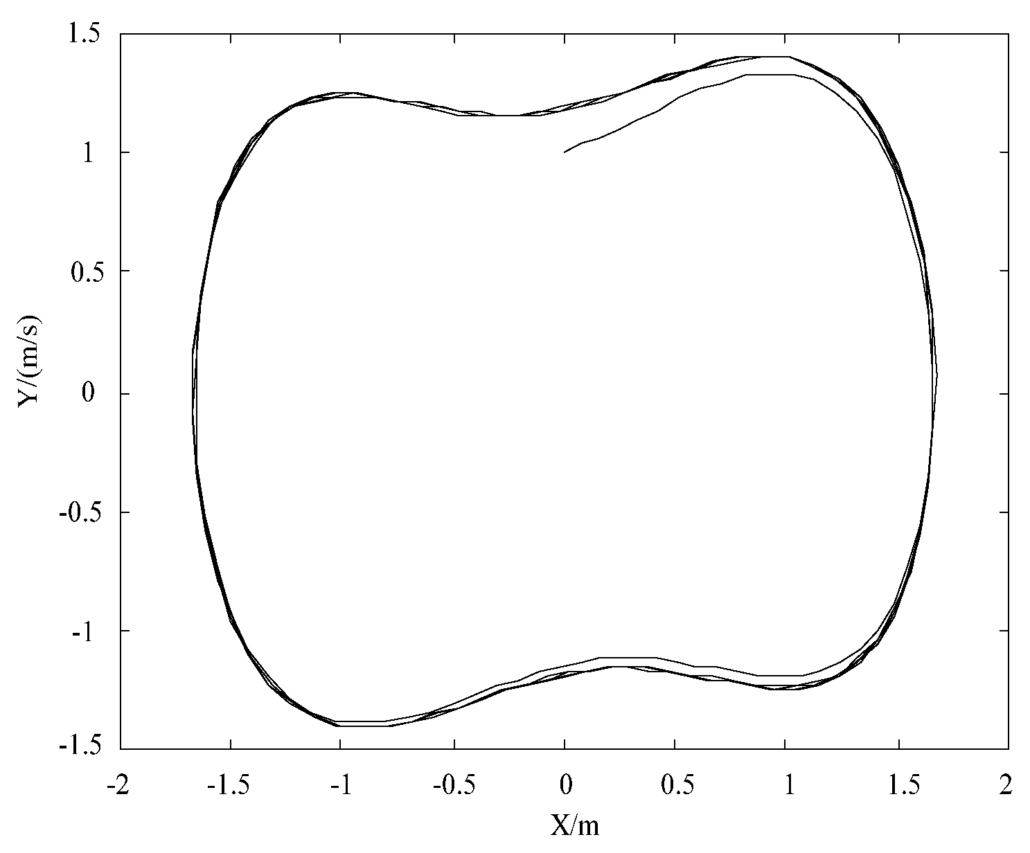
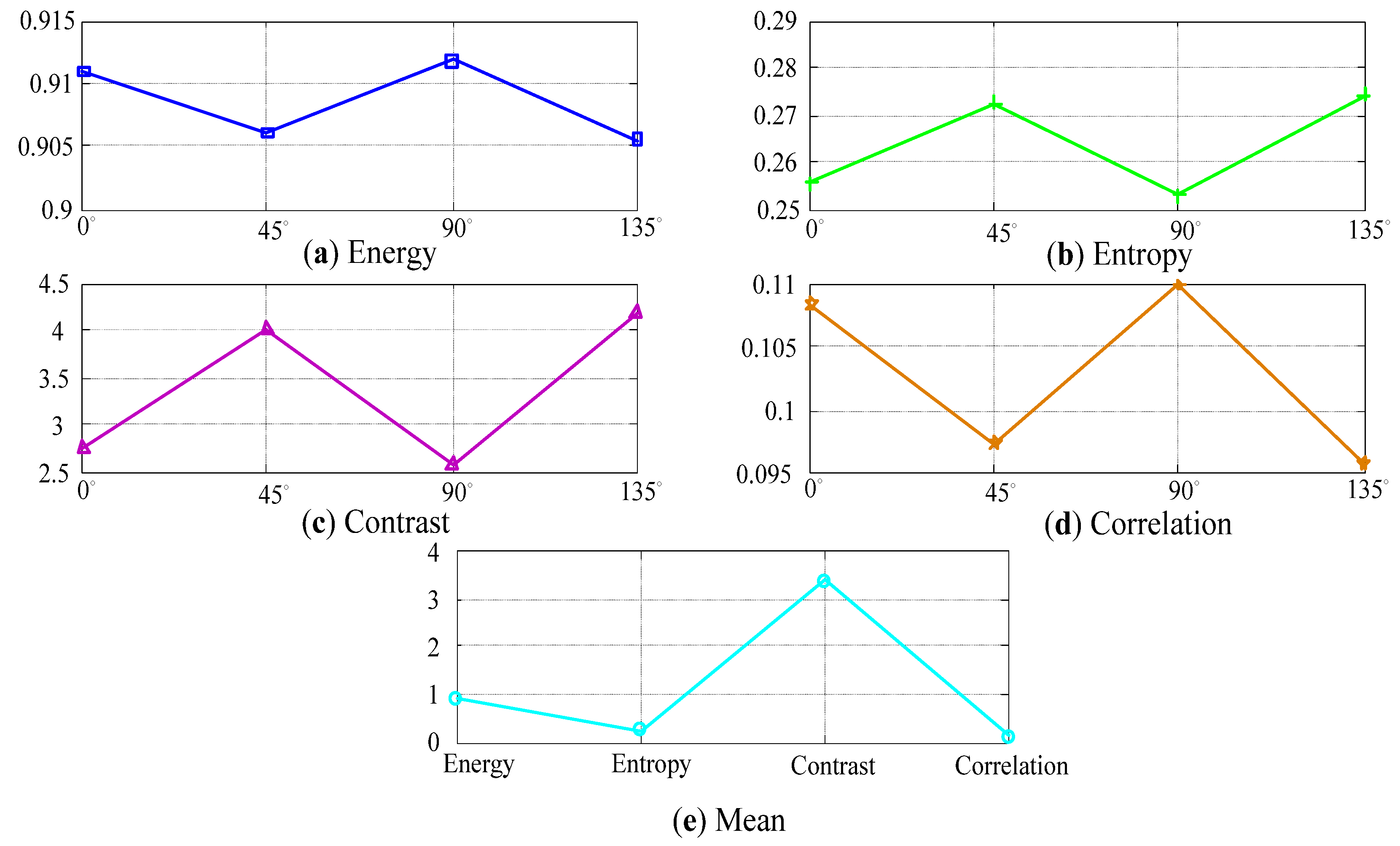
In this paper, a method of automatic recognition of chaotic characteristics based on texture features is proposed. According to this method, we can easily and quickly judge that the system is in a chaotic state or a stable large-scale periodic state. The gray level co-occurrence matrix (GLCM) can describe texture features [39]. We construct the GLCM of four directions [40], namely 0 ° ,   45 ° ,   90 ° , and 135 ° . Energy, entropy, contrast, and correlation [41,42] can be extracted from the four GLCMs. We calculated the mean value of the same feature in four directions. The four texture features were defined as a texture feature vector. The large-scale periodic motion state is shown in Figure 11.
We calculated the texture parameters of this phase diagram. The results are shown in Figure 12. The mean result is defined as the reference vector. We calculated the Euclidean distance between this reference vector and the texture parameter vectors of other phase diagrams. After many experiments, it was concluded that if the Euclidean distance is less than 1.5, the phase diagram is in the large-scale periodic motion state. Otherwise, the phase diagram is in a chaotic state. The method can avoid the involvement of human factors and automatically identify chaotic nature by computers.

6. Fault Line Selection Steps and Simulation

6.1. Introduction of the Fault Line Selection Steps

When a single phase-to-ground fault occurs in the non-solid-earthed network, the system can generate asymmetric zero-sequence currents. The zero-sequence currents of all lines are processed as follows:
Step 1: The zero-sequence current is decomposed by MCEEMD. We can get a series of intrinsic mode functions.
Step 2: The superior filtering algorithm can be selected by the optimal smooth denoising model, and it is used as the input signal of the Duffing system.
Step 3: The Duffing system is adjusted to the critical state. Every line’s denoising result is input into the Duffing system.
Step 4: We calculate the texture parameters of all phase diagrams. The state of the system is judged by Euclidean distance. The phase diagram state of the fault line is different from that of the non-fault line. If all phase diagrams are in the same state, the bus bar is the faulty line.

6.2. Simulation Study

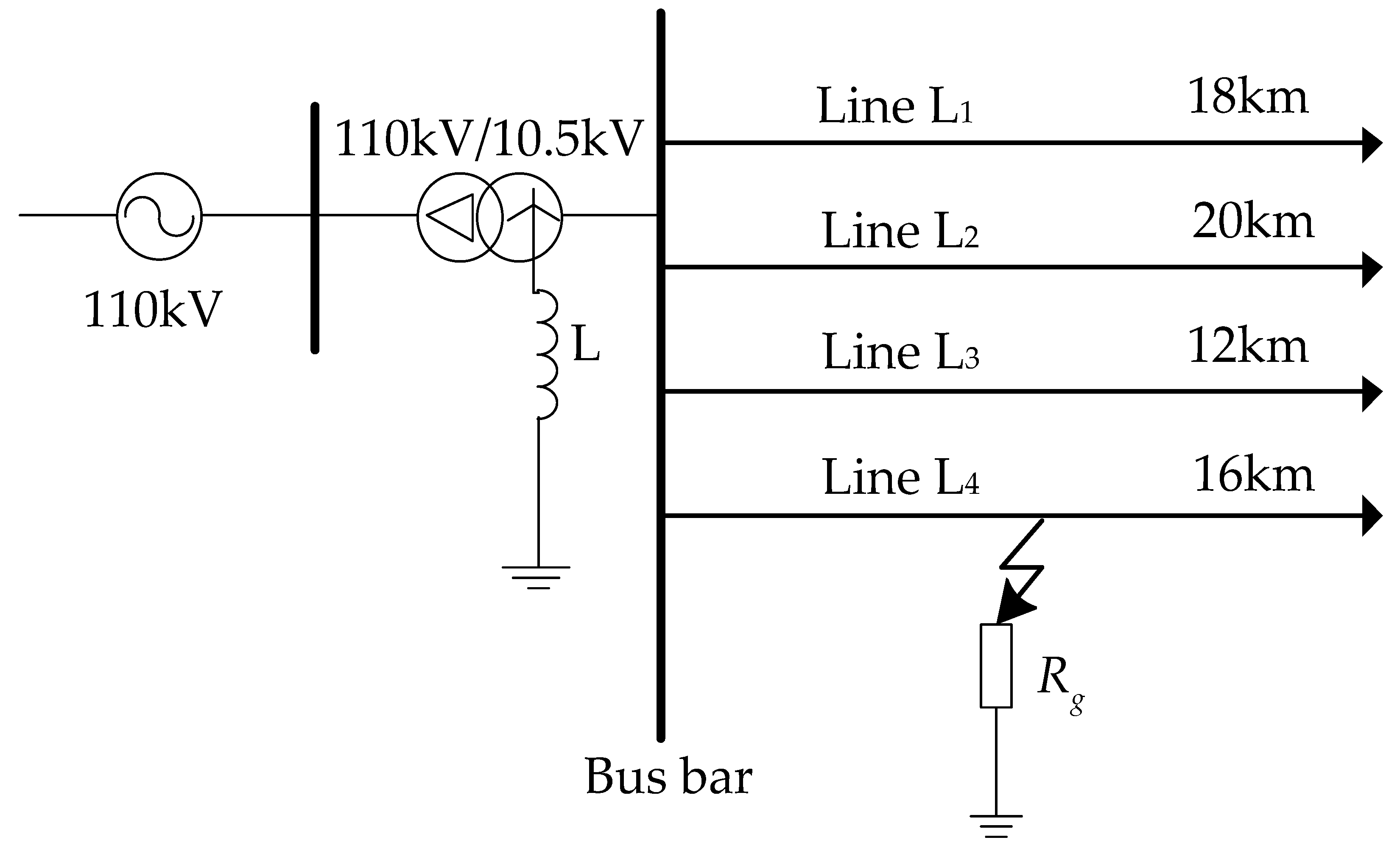
The MATLAB software was used in this paper to simulate the non-solid-earthed network. The simulation model is shown in Figure 13. The three-phase voltage source is set as 110 kV. The transformer ratio is 110 kV/10.5 kV, and its nominal capacity is 20 MVA. Table 6 also shows the impedance parameters and length of the lines. The equivalent inductance of the arc-suppression coil is 1.2102 H.
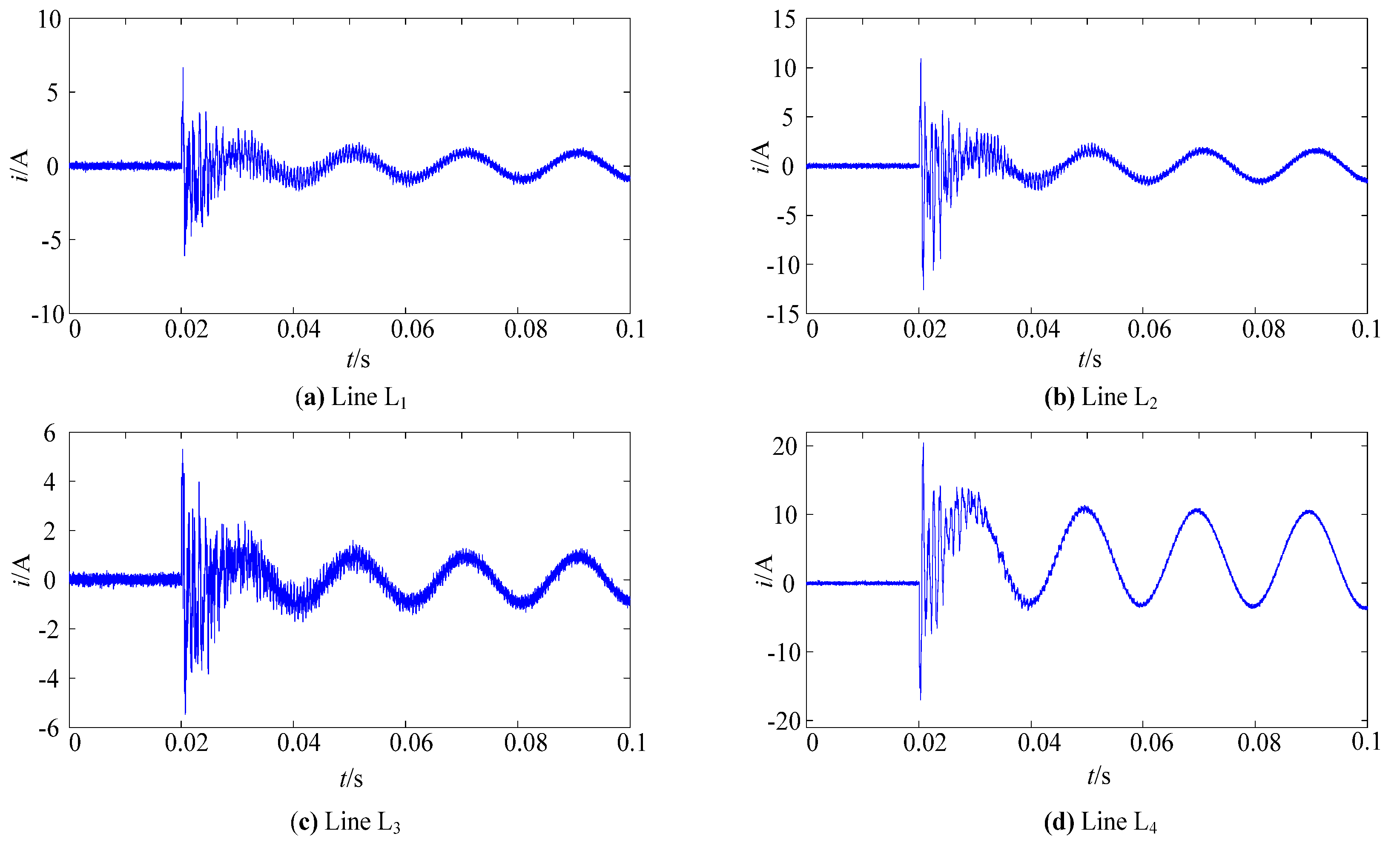
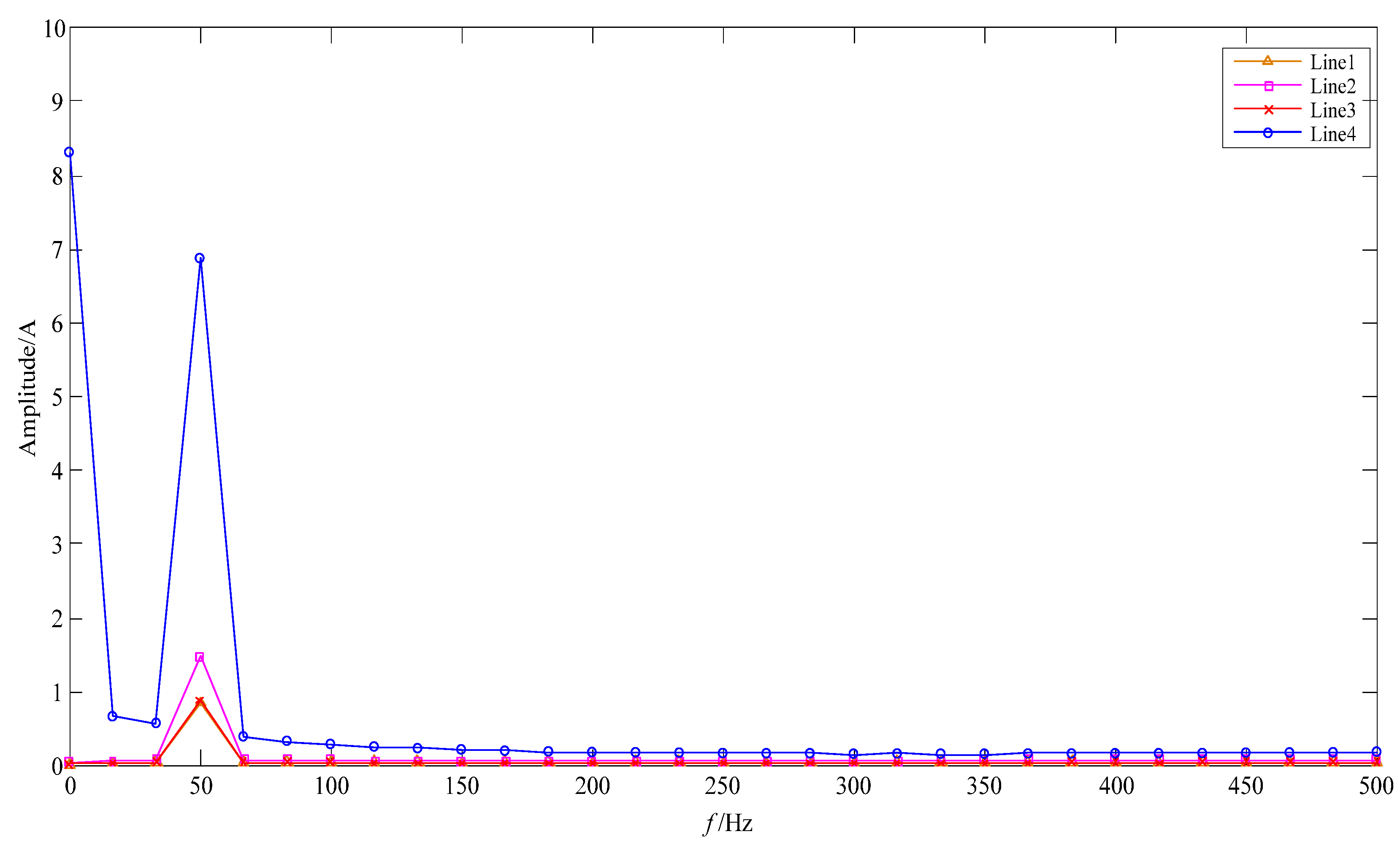
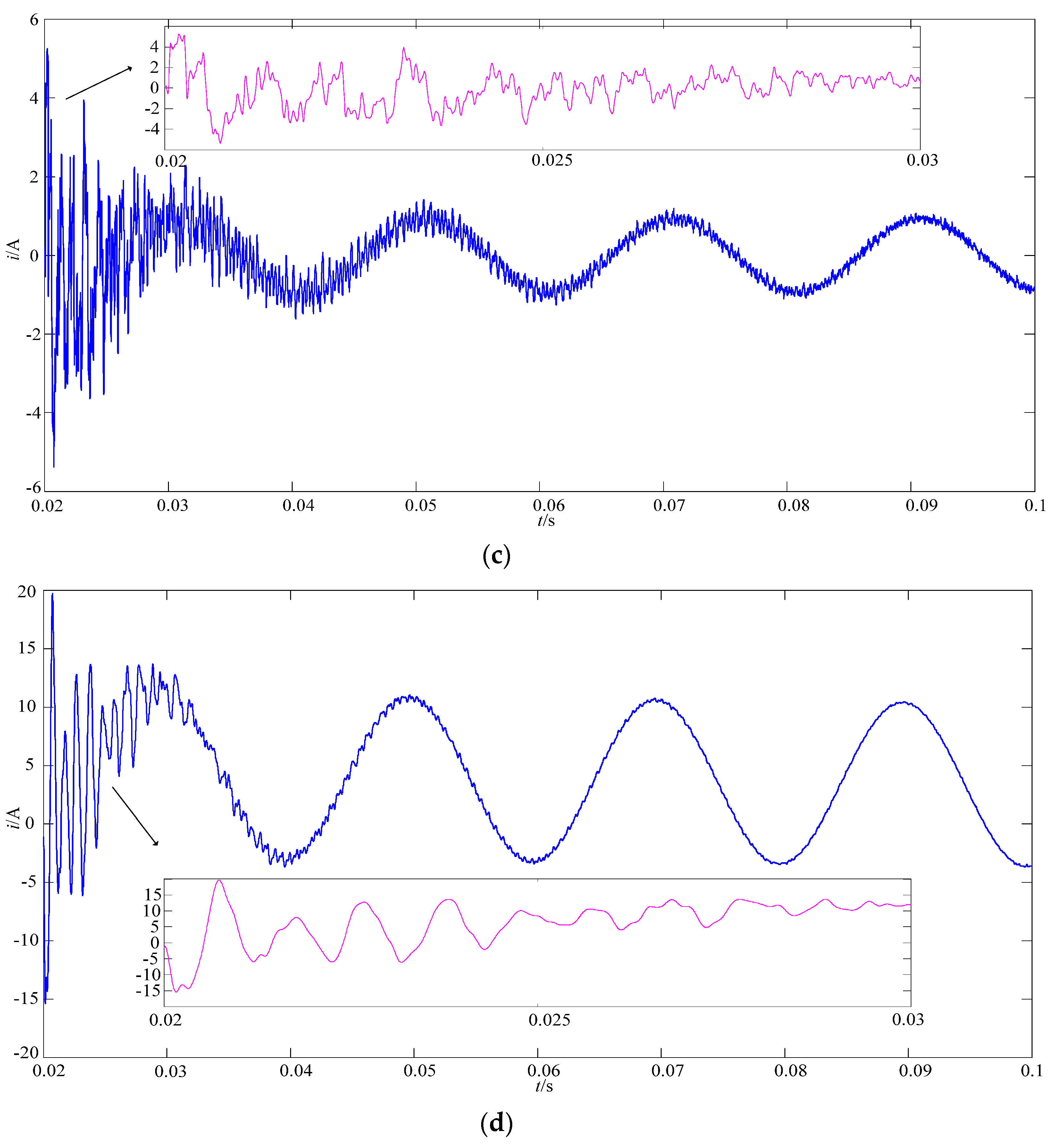
Case 1: Suppose there is a single-phase-to-ground fault in phase A of line L4 at 0.02 s, 5 km away from the bus bar. The ground resistance Rg is 10 Ω. The zero-sequence currents collected in the actual non-solid-earthed network often carry noise with them. After the simulation, we add the Gaussian white noise to the zero-sequence currents in lines 1–4. The results are shown in Figure 14 from 0 to 0.1 s. Every line’s zero-sequence current is done with the help of fast Fourier transform. The result of fast Fourier transform analysis is shown in Figure 15. As seen from Figure 15, the zero-sequence current contains minor amounts of the fifth harmonic. In a study by Zhang and colleagues [8], the method of fault line selection failed by comparing the amplitude of the fifth harmonic.
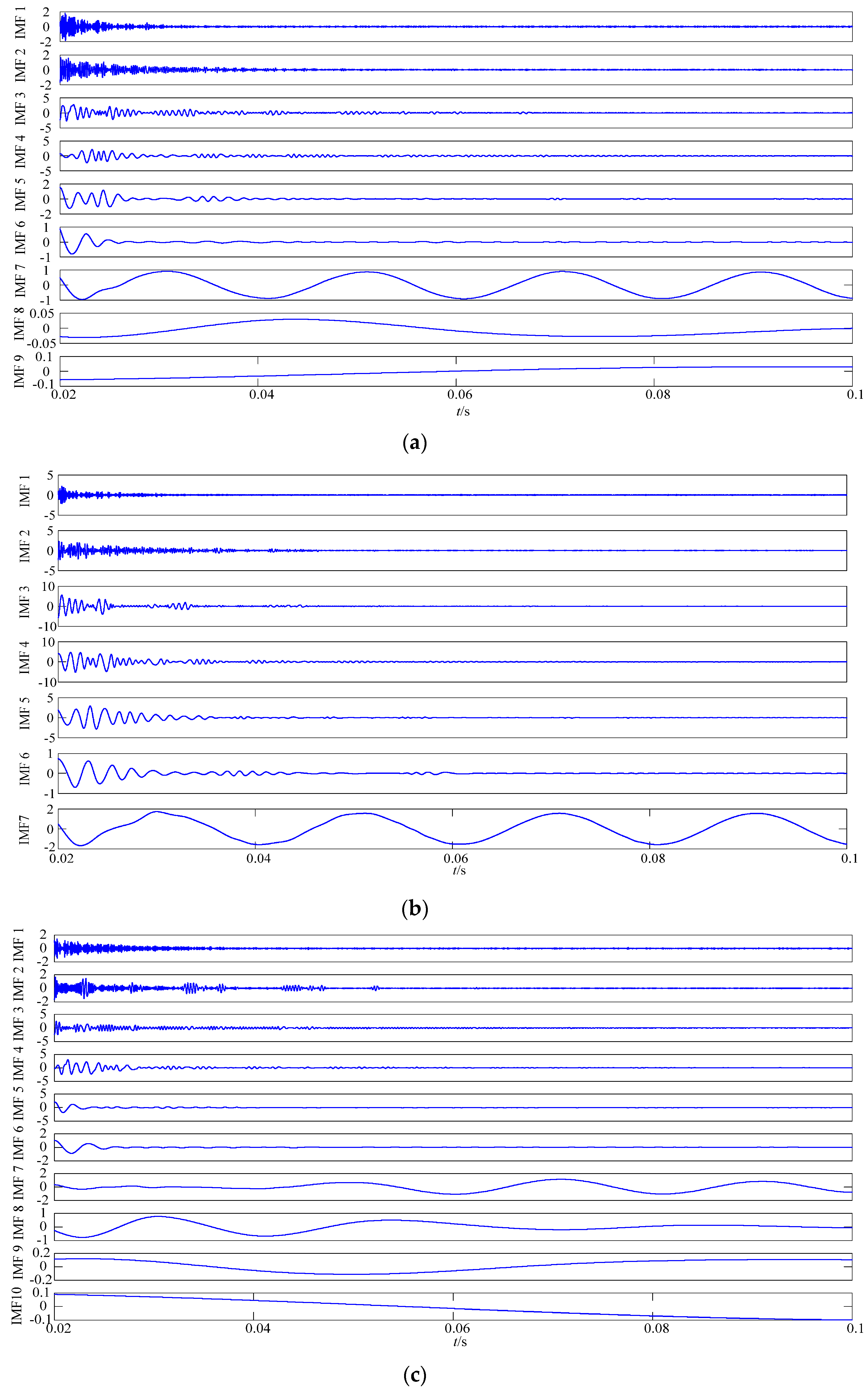
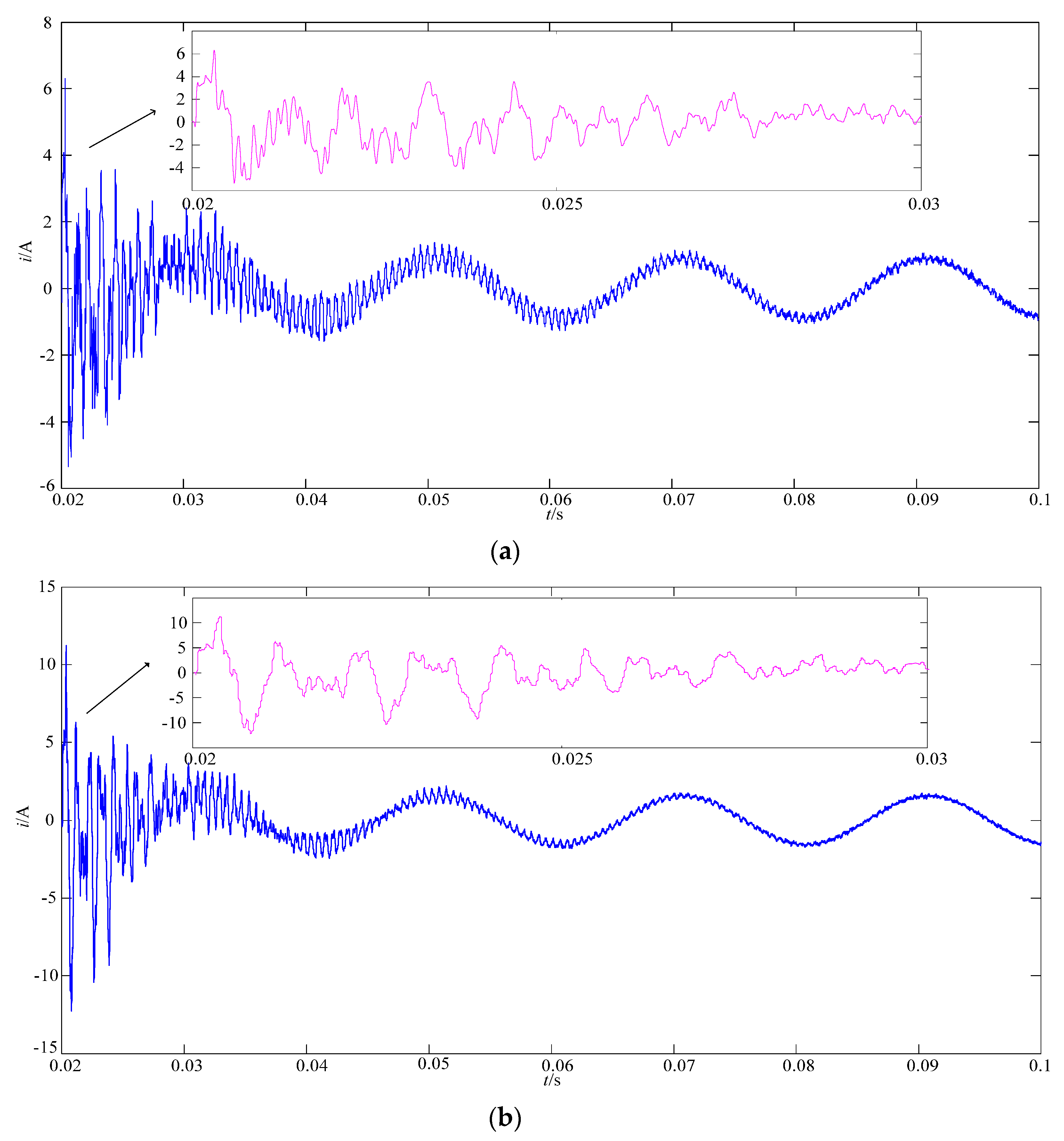
MCEEMD is used to decompose the post-fault zero-sequence current. The decomposition results are shown in Figure 16. As seen from Figure 16, the results of each line are arranged in descending sequence by frequency. Different intrinsic mode functions can be obtained by using MCEEMD, and a series of filtering algorithms can be obtained, respectively. The optimum filtering algorithm can be determined by the optimal smooth denoising model. Every line’s optimal smooth denoising result is shown in Figure 17. As shown in Figure 17, the proposed algorithm not only achieves noise reduction effect, but also reflects well the available information of the original signal. Every line’s denoising result can be used as the input signal of the Duffing system.
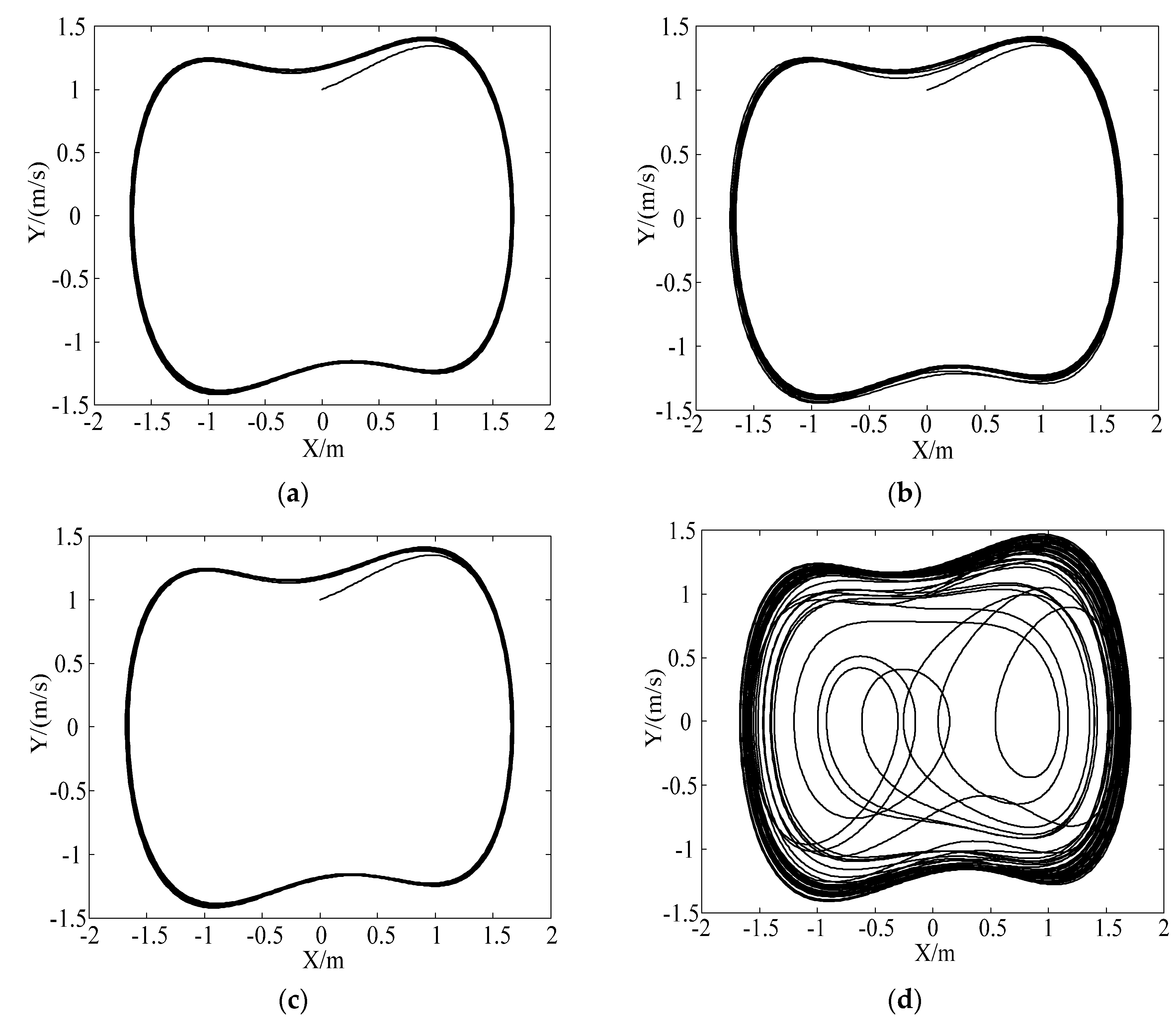
The Duffing system is adjusted to the critical state. Every line’s denoising result is input into the Duffing system. The equation of the Duffing system is solved by the fourth-order Runge–Kutta. The Duffing system’s phase diagram when adding each line’s denoising result is shown in Figure 18. As can be seen in Figure 18, the phase diagram of line L4 is in a chaotic state while the others are in a large-scale periodic motion state. It can be seen that the trajectory of the large-scale periodic motion state moves around (±1, 0) and (0, 0). The fifth harmonic components of the fault line and the non-fault line can make the Duffing system in different state trajectories. Therefore, line L4 has a single-phase-to-ground fault. For automatically identifying chaotic nature, we extract texture features of phase diagrams. As introduced in Section 5.3, the reference vector of the texture feature is (0.9086, 0.2638, 3.3849, 0.1029). The chaotic nature can be identified according to the Euclidean distance between the reference vector and texture feature of the phase diagram. The results are shown in Table 7. As shown in Table 7, only the Euclidean distance of line L4 is more than 1.5, and therefore its phase diagram is in a chaotic state. However, the other phase diagrams are the large-scale periodic state. The results mean the method can select the fault line accurately.
Case 2: Since fault conditions are different in the actual non-solid-earthed network, we carried out different fault situations, such as fault line, fault resistance, and fault distance. The selection results of fault in different conditions are shown in Table 8. As can be seen in Table 8, the Duffing systems of the fault line and the non-fault line show different state trajectories. Table 8 also shows that the state of the system can be accurately identified by the texture feature recognition of the phase diagram. If Euclidean distance is less than 1.5, the phase diagram is the large-scale periodic motion state. Otherwise, the phase diagram is a chaotic state. To summarize, the proposed method is able to select the fault line with different situations.

7. Conclusions

In this paper, we proposed a novel fault line selection method for the non-solid-earthed network based on MCEEMD and the Duffing system, and the research came to the following conclusions:
(1)
GCMPE can solve the deficiencies of MPE and has better stability than MPE. Based on GCMPE and SVM for abnormal signal detection, a new denoising algorithm is proposed. The simulation results show that MCEEMD has better decomposition results than the existing algorithms. MCEEMD also has strong adaptability and restrains the mode mixing of EMD.
(2)
The optimal smooth denoising model can be determined by balancing the similarity and smoothness of different filtering algorithms. The superior algorithm can retain the useful features of the original signal and reduce the noise and smooth the original signal.
(3)
A novel method of identifying chaotic nature based on texture features of the phase diagram is presented. This way can avoid the involvement of human factors and automatically identify chaotic nature by computers.
(4)
The fault line in the non-solid-earthed network can be selected with the diagram outputted by the Duffing system. A large number of experimental studies show that the proposed method can accurately select the fault line under different fault situations. The research provides a novel train of thought for the fault line in the non-solid-earthed network.

Author Contributions

Conceptualization, S.H. and W.G.; methodology, S.H.; software, W.G.; validation, S.H. and W.G.; formal analysis, S.H.; investigation, W.G.; resources, S.H. and W.G.; data curation, W.G.; writing—original draft preparation, S.H. and W.G.; writing—review and editing, W.G.; visualization, S.H. and W.G.; supervision, S.H.; project administration, S.H. All authors have read and agreed to the published version of the manuscript.

Funding

This research received no external funding.

Acknowledgments

This work was supported by the National Key R&D Program of China (Grant no. 2018YFF01011900).

Conflicts of Interest

The authors declare no conflicts of interest.

Nomenclature

MCEEMDModified complementary ensemble empirical mode decomposition
GCMPEGeneralized composite multiscale permutation entropy
SVMSupport vector machine
IMFIntrinsic mode functions
EMDEmpirical mode decomposition
VMDVariational mode decomposition
EEMDEnsemble empirical mode decomposition
CEEMDComplementary ensemble empirical mode decomposition
CEEMDANComplete ensemble empirical mode decomposition with adaptive noise
PEPermutation entropy
MPEMultiscale permutation entropy
GLCMGray level co-occurrence matrix
OrtOrthogonality
FFTFast Fourier transform

References

  1. Wang, X.; Gao, J.; Song, G.; Cheng, Q.; Wei, X.; Wei, Y. Faulty line selection method for distribution network based on variable scale bistable system. J. Sens. 2016, 2016, 7436841. [Google Scholar] [CrossRef] [Green Version]
  2. Wang, X.; Wei, Y.; Zeng, Z.; Hou, Y.; Gao, J.; Wei, X. Fault line selection method of small current to ground system based on atomic sparse decomposition and extreme learning machine. J. Sens. 2015, 2015, 678120. [Google Scholar] [CrossRef]
  3. Shao, W.; Bai, J.; Cheng, Y.; Zhang, Z.; Li, N. Research on a faulty line selection method based on the zero-sequence disturbance power of resonant grounded distribution networks. Energies 2019, 12, 846. [Google Scholar] [CrossRef] [Green Version]
  4. Lin, X.; Sun, J.; Kursan, I.; Zhao, F.; Li, Z.; Li, X.; Yang, D. Zero-sequence compensated admittance based faulty feeder selection algorithm used for distribution network with neutral grounding through Peterson-coil. Int. J. Electr. Power Energy Syst. 2014, 63, 747–752. [Google Scholar] [CrossRef]
  5. Zhuang, S.; Miao, X.; Jiang, H.; Guo, M. A line selection method for single-phase high-impedance grounding fault in resonant grounding system of distribution network based on improved euclidean-dynamic time warping distance. Power Syst. Technol. 2020, 44, 273–281. [Google Scholar]
  6. Dong, X.; Shi, S. Identifying single-phase-to-ground fault feeder in neutral noneffectively grounded distribution system using wavelet transform. IEEE Trans. Power Deliv. 2008, 23, 1829–1837. [Google Scholar] [CrossRef]
  7. Costa, F.; Souza, B.; Brito, N.; Silva, J.; Santos, W. Real-time detection of transients induced by high-impedance faults based on the boundary wavelet transform. IEEE Trans. Ind. Appl. 2015, 51, 5312–5323. [Google Scholar] [CrossRef]
  8. Zhang, Z.; Liu, X.; Piao, Z. Fault line detection in neutral point ineffectively grounding power system based on phase-locked loop. IET Gener. Transm. Distrib. 2014, 8, 273–280. [Google Scholar]
  9. Zhang, S.; Zhai, X.; Dong, X.; Li, L.; Tang, B. Application of EMD and Duffing oscillator to fault line detection in un-effectively grounded system. Proc. Chin. Soc. Electr. Eng. 2013, 33, 161–167. [Google Scholar]
  10. Kang, X.; Liu, X.; Suonan, J.; Ma, C.; Wang, C.; Yang, L. New method for fault line selection in non-solidly grounded system based on matrix pencil method. Autom. Electr. Power Syst. 2012, 36, 88–93. [Google Scholar]
  11. Li, Y.; Li, Y.; Chen, X.; Yu, J. Denoising and feature extraction algorithms using NPE combined with VMD and their applications in ship-radiated noise. Symmetry 2017, 9, 256. [Google Scholar] [CrossRef] [Green Version]
  12. Hou, J.; Wu, Y.; Gong, H.; Ahmad, A.; Liu, L. A novel intelligent method for bearing fault diagnosis based on EEMD permutation entropy and GG clustering. Appl. Sci. 2020, 10, 386. [Google Scholar] [CrossRef] [Green Version]
  13. Wang, S.; Sun, Y.; Zhou, Y.; Jamil Mahfoud, R.; Hou, D. A new hybrid short-term interval forecasting of PV output power based on EEMD-SE-RVM. Energies 2019, 13, 87. [Google Scholar] [CrossRef] [Green Version]
  14. Xue, S.; Tan, J.; Shi, L.; Deng, J. Rope tension fault diagnosis in hoisting systems based on vibration signals using EEMD, improved permutation entropy, and PSO-SVM. Entropy 2020, 22, 209. [Google Scholar] [CrossRef] [Green Version]
  15. Ren, Y.; Suganthan, P.; Srikanth, N. A comparative study of empirical mode decomposition-based short-term wind speed forecasting methods. IEEE Trans. Sustain. Energy 2015, 6, 236–244. [Google Scholar] [CrossRef]
  16. Zhao, L.; Yu, W.; Yan, R. Rolling bearing fault diagnosis based on CEEMD and time series modeling. Math. Probl. Eng. 2014, 2014, 101867. [Google Scholar] [CrossRef]
  17. Liu, F.; Gao, J.; Liu, H. The feature extraction and diagnosis of rolling bearing based on CEEMD and LDWPSO-PNN. IEEE Access 2020, 8, 19810–19819. [Google Scholar] [CrossRef]
  18. Yang, D.; Sun, Y.; Wu, K. Research on CEEMD-AGA denoising method and its application in feed mixer. Math. Probl. Eng. 2020, 2020, 9873268. [Google Scholar] [CrossRef]
  19. Fuentealba, P.; Illanes, A.; Ortmeier, F. Independent analysis of decelerations and resting periods through CEEMDAN and spectral-based feature extraction improves cardiotocographic assessment. Appl. Sci. 2019, 9, 5421. [Google Scholar] [CrossRef] [Green Version]
  20. Li, G.; Yang, Z.; Yang, H. A denoising method of ship radiated noise signal based on modified CEEMDAN, dispersion entropy, and interval thresholding. Electronics 2019, 8, 597. [Google Scholar] [CrossRef] [Green Version]
  21. Tian, S.; Bian, X.; Tang, Z.; Yang, K.; Li, L. Fault diagnosis of gas pressure regulators based on CEEMDAN and feature clustering. IEEE Access 2019, 7, 132492–132502. [Google Scholar] [CrossRef]
  22. Wang, G.; Chen, D.; Lin, J.; Chen, X. The application of chaotic oscillators to weak signal detection. IEEE Trans. Ind. Electron. 1999, 46, 440–444. [Google Scholar] [CrossRef]
  23. Xue, W.; Dai, X.; Zhu, J.; Luo, Y.; Yang, Y. A noise suppression method of ground penetrating radar based on EEMD and permutation entropy. IEEE Geosci. Remote Sens. Lett. 2019, 16, 1625–1629. [Google Scholar] [CrossRef]
  24. Srinu, S.; Mishra, A.K. Cooperative sensing based on permutation entropy with adaptive thresholding technique for cognitive radio networks. IET Sci. Meas. Technol. 2016, 10, 934–942. [Google Scholar] [CrossRef]
  25. Du, W.; Guo, X.; Wang, Z.; Wang, J.; Yu, M.; Li, C.; Wang, G.; Wang, L.; Guo, H.; Zhou, J.; et al. A new fuzzy logic classifier based on multiscale permutation entropy and its application in bearing fault diagnosis. Entropy 2019, 22, 27. [Google Scholar] [CrossRef] [Green Version]
  26. Wang, X.; Lu, Z.; Wei, J.; Zhang, Y. Fault diagnosis for rail vehicle axle-box bearings based on energy feature reconstruction and composite multiscale permutation entropy. Entropy 2019, 21, 865. [Google Scholar] [CrossRef] [Green Version]
  27. Huo, Z.; Zhang, Y.; Shu, L.; Gallimore, M. A new bearing fault diagnosis method based on fine-to-coarse multiscale permutation entropy, laplacian score and SVM. IEEE Access 2019, 7, 17050–17066. [Google Scholar] [CrossRef]
  28. Humeau-Heurtier, A.; Wu, C.-W.; Wu, S.-D. Refined composite multiscale permutation entropy to overcome multiscale permutation entropy length dependence. IEEE Signal Process. Lett. 2015, 22, 2364–2367. [Google Scholar] [CrossRef]
  29. Zheng, J.; Liu, T.; Meng, R.; Liu, Q. Generalized composite multiscale permutation entropy and PCA based fault diagnosis of rolling bearings. J. Vib. Shock 2018, 37, 61–66. [Google Scholar]
  30. Wan, Z.; Yi, S.; Li, K.; Tao, R.; Gou, M.; Li, X.; Guo, S. Diagnosis of elevator faults with LS-SVM based on optimization by K-CV. J. Electr. Comput. Eng. 2015, 2015, 935038. [Google Scholar] [CrossRef] [Green Version]
  31. Liu, W.; Zhou, X.; Jiang, Z.; Ma, F. Improved empirical mode decomposition method based on optimal feature. J. Jilin Univ. (Eng. Tech. Ed.) 2017, 47, 1957–1963. [Google Scholar]
  32. Wang, Z.; Qiao, P.; Shi, B. Nonpenetrating damage identification using hybrid lamb wave modes from Hilbert-Huang spectrum in thin-walled structures. Shock Vib. 2017, 2017, 5164594. [Google Scholar] [CrossRef] [Green Version]
  33. Zheng, Y.; Sun, X.; Chen, J.; Yue, J. Extracting pulse signals in measurement while drilling using optimum denoising methods based on the ensemble empirical mode decomposition. Pet. Explor. Dev. 2012, 39, 750–753. [Google Scholar] [CrossRef]
  34. Li, G.; Zeng, L.; Zhang, L.; Wu, Q. State identification of Duffing oscillator based on extreme learning machine. IEEE Signal Process. Lett. 2018, 25, 25–29. [Google Scholar] [CrossRef]
  35. Song, W.; Deng, S.; Yang, J.; Cheng, Q. Tool wear detection based on Duffing-holmes oscillator. Math. Probl. Eng. 2008, 2008, 510406. [Google Scholar] [CrossRef] [Green Version]
  36. Chang, T. Chaotic motion in forced Duffing system subject to linear and nonlinear damping. Math. Probl. Eng. 2017, 2017, 3769870. [Google Scholar] [CrossRef]
  37. Li, Y.; Yang, B.; Shi, Y. Chaos-based weak sinusoidal signal detection approach under colored noise background. Acta Phys. Sin. Chin. Ed. 2003, 52, 526–530. [Google Scholar]
  38. Shang, Q.; Yin, C.; Li, S.; Yang, Y. Study on detection of weak sinusoidal signal by using Duffing oscillator. Proc. Chin. Soc. Electr. Eng. 2005, 25, 66–70. [Google Scholar]
  39. Suresh, A.; Shunmuganathan, K.L. Image texture classification using gray level co-occurrence matrix based statistical features. Eur. J. Sci. Res. 2012, 75, 591–597. [Google Scholar]
  40. Luo, J.; Song, D.; Xiu, C.; Geng, S.; Dong, T. Fingerprint classification combining curvelet transform and gray-level cooccurrence matrix. Math. Probl. Eng. 2014, 2014, 592928. [Google Scholar] [CrossRef]
  41. Liu, X.; Xu, K.; Zhou, P.; Liu, H. Feature extraction with discrete non-separable shearlet transform and its application to surface inspection of continuous casting slabs. Appl. Sci. 2019, 9, 4668. [Google Scholar] [CrossRef] [Green Version]
  42. Lo, C.; Chen, C.; Yeh, Y.; Chang, C.; Yeh, H. Quantitative analysis of melanosis coli colonic mucosa using textural patterns. Appl. Sci. 2020, 10, 404. [Google Scholar] [CrossRef] [Green Version]
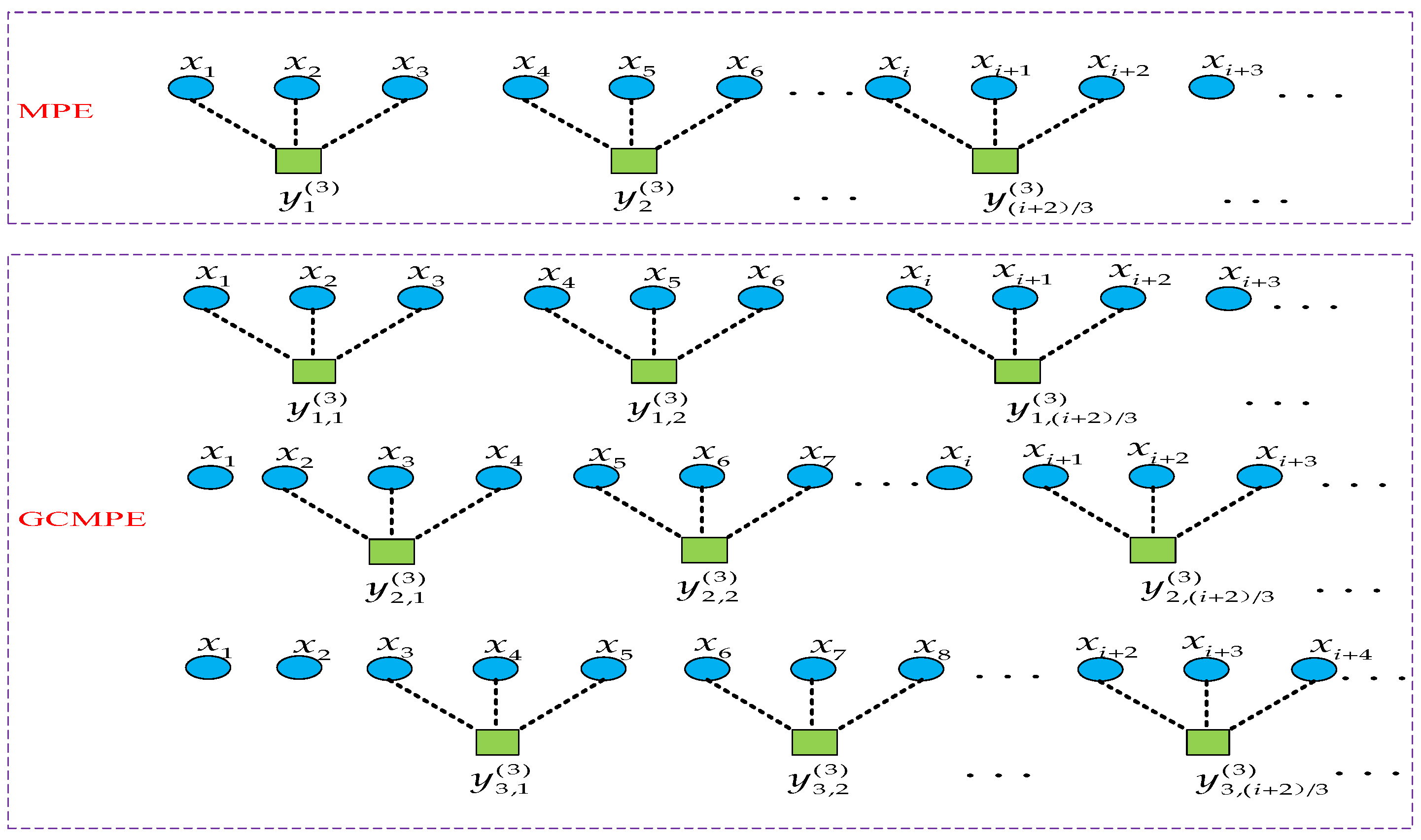
Figure 1. The coarse granulation’s processes of multiscale permutation entropy and generalized composite multiscale permutation entropy with s = 3.
Symmetry 12 00536 g001
Figure 2. Multiscale permutation entropy (MPE) and generalized composite multiscale permutation entropy (GCMPE) of white noise under different scale factors and embedded dimensions [26].
Symmetry 12 00536 g002
Figure 3. GCMPE values for various types of signals.
Symmetry 12 00536 g003
Figure 4. Original simulation signals.
Symmetry 12 00536 g004
Figure 5. The decomposition results of (a) empirical mode decomposition (EMD), (b) complementary ensemble empirical mode decomposition (CEEMD), and (c) modified complementary ensemble empirical mode decomposition (MCEEMD).
Symmetry 12 00536 g005aSymmetry 12 00536 g005b
Figure 6. Hilbert–Huang spectrum of (a) EMD, (b) CEEMD, and (c) MCEEMD.
Symmetry 12 00536 g006
Figure 7. Simulation signals. (a) The clear signal. (b) The noisy signal.
Symmetry 12 00536 g007
Figure 8. The MCEEMD results of simulation signal x.
Symmetry 12 00536 g008
Figure 9. The denoising results for different methods. (a) The denoising result of the wavelet threshold denoising. (b) The denoising result of the optimal smooth denoising model.
Symmetry 12 00536 g009
Figure 10. The detection process of trisection symmetry phase estimation (TSPE).
Symmetry 12 00536 g010
Figure 11. Large-scale periodic motion state.
Symmetry 12 00536 g011
Figure 12. The results for texture parameters. (a) Energy result; (b) entropy result; (c) contrast result; (d) correlation result; (e) mean result.
Symmetry 12 00536 g012
Figure 13. Simulation model of the non-solid-earthed network.
Symmetry 12 00536 g013
Figure 14. Every line’s zero-sequence current with noise. (a) The result of line L1; (b) the result of line L2; (c) the result of line L3; (d) the result of line L4.
Symmetry 12 00536 g014
Figure 15. The result of fast Fourier transform analysis.
Symmetry 12 00536 g015
Figure 16. Every line’s decomposition result. The results of (a) line L1, (b) line L2, (c) line L3; (d) line L4.
Symmetry 12 00536 g016aSymmetry 12 00536 g016b
Figure 17. Every line’s optimal smooth denoising result. (a) line L1 after denoising; (b) line L2 after denoising; (c) line L3 after denoising; (d) line L4 after denoising.
Symmetry 12 00536 g017aSymmetry 12 00536 g017b
Figure 18. Duffing system’s phase diagram when adding each line’s denoising result. The phase diagram of (a) line L1, (b) line L2, (c) line L3, and (d) line L4.
Symmetry 12 00536 g018
Table 1. The correlation coefficients of EMD decomposition. IMF: intrinsic mode functions.
x1x2x3
IMF10.90310.00090.0489
IMF20.28890.47600.0214
IMF30.00190.37900.0246
IMF4−0.00200.3267−0.0277
IMF50.00070.0061−0.0103
IMF60.0010−0.00300.0105
IMF70.0001−0.0004−0.0012
IMF80.0032−0.0010−0.0088
Table 2. The correlation coefficients of CEEMD decomposition.
x1x2x3
IMF10.3952−0.00580.7078
IMF20.9993−0.0035−0.0107
IMF30.03690.9804−0.0156
IMF40.00050.9475−0.0183
IMF5−0.00110.2294−0.0149
IMF6−0.00240.0257−0.0005
IMF7−0.00280.0085−0.0006
Table 3. The correlation coefficients of MCEEMD decomposition.
x1x2x3
IMF10.99950.00080.0235
IMF2−0.00100.9992−0.0092
Table 4. The index of orthogonality (Ort).
Denoising AlgorithmsOrt
EMD0.0891
CEEMD0.0671
MCEEMD 5.8701 × 10 5
Table 5. Amse, Asmse, and Aminf for different filtering algorithms.
Filtering AlgorithmsAmseAsmseAminf
SR10.6597100.0163830.402380
SR20.2742790.0165120.171172
SR30.1583270.0165050.101598
SR40.1251000.0165050.081662
SR50.1096980.0165050.072421
SR60.1092620.0165050.072159
SR70.1092050.0165050.072125
SR80.1069140.0165050.070750
Table 6. The impedance parameters and length of the lines.
LineSequenceResistance
(Ω/km)
Inductance
(mH/km)
Capacitance
(μF/km)
Length
(km)
L1positive-sequence0.18201.11800.115018
zero-sequence0.32505.68100.0096
L2positive-sequence0.12601.01800.120020
zero-sequence0.28504.56000.0150
L3positive-sequence0.18002.15800.129012
zero-sequence0.27305.56100.0150
L4positive-sequence0.13202.22500.229016
zero-sequence0.23805.56100.0235
Table 7. Texture feature and Euclidean distance of phase diagram.
LineEnergyEntropyContrastCorrelationEuclidean DistanceChaotic Nature
L10.92150.22622.07050.12251.3151Periodical
L20.89320.28172.50230.08850.8831Periodical
L30.92250.22422.06890.12461.3168Periodical
L40.62220.827011.93380.02458.5726Chaotic
Table 8. Selection results of fault in different situations.
Fault SituationLineEnergyEntropyContrastCorrelationEuclidean DistanceChaotic NatureResult
(L4,
30 Ω,
10 km)
L10.91720.23522.14170.11531.2436PeriodicalL4
L20.90170.26652.14560.09671.2393Periodical
L30.91550.23952.12110.11381.2641Periodical
L40.62160.819510.85190.02457.4935Chaotic
(L4,
500 Ω,
2 km)
L10.89620.27662.04620.09161.3388PeriodicalL4
L20.85390.34702.22180.06361.1680Periodical
L30.89430.27912.00820.08981.3769Periodical
L40.58180.919915.26760.021711.9056Chaotic
(L4,
1000 Ω,
1 km)
L10.90370.26162.15460.09891.2303PeriodicalL4
L20.87470.31192.01040.07481.3760Periodical
L30.90290.26422.16410.09801.2208Periodical
L40.57350.928915.07230.021311.7144Chaotic
(L3,
200 Ω,
6 km)
L10.92710.21572.29600.13211.0905PeriodicalL3
L20.89990.28915.14980.08761.7652Periodical
L30.61550.840611.94490.02408.5848Chaotic
L40.91490.24022.10990.11261.2552Periodical
(L2,
10 Ω,
3 km)
L10.92120.22772.10770.12211.2779PeriodicalL2
L20.57210.931015.01840.021311.6578Chaotic
L30.92250.22502.06690.12481.3188Periodical
L40.88740.29752.43830.08420.9476Periodical
(L2,
100 Ω,
5 km)
L10.92670.21622.26030.13071.1261PeriodicalL2
L20.61570.844412.44700.02409.0858Chaotic
L30.92650.21672.26890.13101.1166Periodical
L40.87750.33384.78630.07531.4038Periodical
(L2,
600 Ω,
1 km)
L10.92700.21602.34710.13151.0394PeriodicalL2
L20.76120.56357.05960.03893.6905Chaotic
L30.92720.21662.33730.13211.4092Periodical
L40.92010.22982.27780.11991.1077Periodical
(L1,
100 Ω,
3 km)
L10.68060.71369.36710.02916.0039ChaoticL1
L20.91650.23712.06410.11521.3211Periodical
L30.92510.22042.23270.12931.1534Periodical
L40.91350.24242.04840.11071.3367Periodical
(L1,
300 Ω,
12 km)
L10.68800.70589.46380.03006.0994ChaoticL1
L20.93060.20932.43370.13830.9536Periodical
L30.92780.21372.34550.13131.0412Periodical
L40.91720.23632.13880.11611.2465Periodical
(Bus bar,
200 Ω)
L10.92680.21572.29520.13081.0912PeriodicalBus bar
L20.93160.20662.39190.13970.9955Periodical
L30.92680.21662.30390.13091.0825Periodical
L40.91600.23752.07750.11411.3077Periodical
(Bus bar,
1000 Ω)
L10.92850.21332.35960.13391.0272PeriodicalBus bar
L20.92460.22082.35150.12741.0347Periodical
L30.92800.21432.39480.13300.9920Periodical
L40.92270.22472.28170.12341.1041Periodical