Attentive Gated Graph Neural Network for Image Scene Graph Generation

Abstract

Image scene graph is a semantic structural representation which can not only show what objects are in the image, but also infer the relationships and interactions among them. Despite the recent success in object detection using deep neural networks, automatically recognizing social relations of objects in images remains a challenging task due to the significant gap between the domains of visual content and social relation. In this work, we translate the scene graph into an Attentive Gated Graph Neural Network which can propagate a message by visual relationship embedding. More specifically, nodes in gated neural networks can represent objects in the image, and edges can be regarded as relationships among objects. In this network, an attention mechanism is applied to measure the strength of the relationship between objects. It can increase the accuracy of object classification and reduce the complexity of relationship classification. Extensive experiments on the widely adopted Visual Genome Dataset show the effectiveness of the proposed method.

1. Introduction

As the object detection performance improves year by year, these models such as Faster R-CNN [1] and YOLO [2] have made significant progress in detecting individual objects separately. However, we are still far from reaching the goal of capturing the interactions and relationships between these objects. In recent years, researchers have focused more on recognition of more diverse and structured concepts from an image, in the form of scene graph [3,4,5,6]. This aims at capturing the semantic information in an image including the objects entities and pair-wise relationships. Due to its ability of enriching visual semantic analysis, scene graph has been shown to benefit various high-level vision tasks such as image retrieval [7], image caption [8,9], image generation [10] and visual question answering [11]. To truly take advantage of the properties of scene graph, it is crucial to devise a model that automatically generates scene graphs from images.

In a scene graph, the nodes represent either an object, an attribute for an object, or a relationship between two objects. The edges depict the connection and association between two nodes, as shown in Figure 1. Previous scene graph generation methods generally decompose the scene into triplets in the form <subject-predicate-object>, like <girl-feeding-elephant>, in which predicate represents the interaction between objects with direction. There exist various kinds of interactions between objects, including some verbs (e.g., taking, feeding), comparatives (e.g., bigger, smaller), positions (e.g., above, behind). As such, a scene graph is able to model not only what objects are in the scene, but also how they relate to each other.

The major challenge of generating scene graphs is recognizing objects in image and reasoning about relationships. Previous attempts have been expended on localizing and recognizing semantic relationships in images [3,5,13,14]. They generally follow the same route. First, the bounding boxes and high-level semantic features of objects are given by object detection network. Second, the relationships are recognition by neural network using the spatial information and features of objects. However, most methods only focus on local prediction, and ignore the global information of surrounding context in images. Yang et al. [3] captures the global context by graph convolutional network, which can propagate information in both directions between objects and relations. Xu et al. [13] attempts to solves the scene graph inference problem using standard Recurrent Neural Networks (RNNs) and learns to iteratively improves its predictions via message passing. Although they extract the global information by different manners, the extraction module cannot automatically select effective global information. Thus, the accuracy of object and relation classification will be affected by the redundant information.

In this work, we propose an Attentive Gated Graph Neural Network (AGGNN) to simultaneously recognize objects and filter the redundant information. The gated graph neural network is built by recurrent sequential architectures such as Graph Long Short-term Memory Network (GLSTM). The nodes in GLSTM represent the objects in image while edges can be regarded as relationships among objects. The gated operation can simulate the message propagation in the graph. The attention mechanism changes the message flow ability of the edge by setting importance to different relationships. It can effectively filter redundant information and improve the accuracy of object classification, while reduce the complexity of relationship classification by relationship edge pruning. AGGNN can be jointly trained with object detector and relationship classifier by standard back-propagation methods.

We summarize our contributions as the following: (a) we present a gated graph neural network to model the scene graph, which improves the ability of the model to extract the global context of the image. (b) We integrate attention mechanism into gated graph neural network. It not only improves the accuracy of object classification, but also prunes the redundant relationships in the scene graph. (c) In the relationship classification stage, we extract the global context of relationship by graph feature embedding. It is the input of relationship classifier together with spatial information and semantic features of objects. (d) We compare our model with existing approaches on standard metrics. The results show that our model has a superior performance than the state-of-the-art techniques.

The rest of the paper is structured as follows. Section 2 gives a brief review of related works. Section 3 explains the detail of the AGGNN model. Experimental results and comparisons are shown in Section 4. In Section 5, conclusion remarks and potential directions for the future research are presented.

2. Related Work

Visual Relationship Modeling. Visual relationship detection is a typical method to infer the relationship between each object pair in an image. In the early stage, most of the works focused on a few specific types of visual relations, such as spatial relations (i.e., ’below’, ’above’, and ’inside’) [15,16] and actions [17]. However, these simple phrases cannot represent such complex relationships in an image. General visual relationship detection has been paid more attention [18,19,20], where the subject and object can be any objects in the image and their relationships cover a wide range of relationship types. These methods generally adopt a neural network to classify the relationship by using bounding boxes and semantic features of subject and object as the input. Lu et al. [18] uses language model to enhance the ability of relationship classification by word embedding. It can be simply understood that the samples which have seen are mainly used for prediction by visual model, and the samples which have not seen are mainly used for prediction by language model. However, these works only focus on the local information and cannot learn the global structural representation of an image. Recently, increasingly more researchers put their attention on interactions between image and language. Language description has the advantage over a simple label prediction in that the output naturally encodes the structure of various concepts, such as a relationship between objects [21,22,23]. They rely on a so-called encoder–decoder model, in which a deep Convolutional Neural Network (CNN) is pretrained as the encoder to extract image features, and then LSTM with language model decodes the features into some sentences. These methods mainly to get the object categories and simple object relationships in the visual data, and its effect is often poor for scenes with complex relationships. In addition, the semi-structured text is dynamic and variable, which makes it impossible for the computer to process such data directly.

Image Scene Graph Generation. Scene graph generation is a task derived from Visual Relationship modeling. As a type of structured data, scene graph can uniquely represent an image. After Krishna et al. [12] proposed large-scale visual genome dataset for scene graph reasoning, more and more researchers began to use Deep Neural Network (DNN) method to construct scene graph. At present, image scene graph generation can be divided into two categories. First, the early methods [24,25] are to separate the object classification and the relationship classification. After using the region proposal networks [1] to get the object classification, the relationship is classified by combining the depth semantic features of objects. Second, the recent methods take object classification and relation classification as a whole. After using the region proposal network to extract the object proposals, the feature fusion of the two classification tasks is realized by using the message passing mechanism, and the categories of objects and relationships will output finally. Xu et al. [13] initialized a fully connected scene graph, and divided the nodes and edges of the graph into two categories. Then they used two RNNs to pass the message iteratively, and finally generate the scene graph under the condition of distance constraint. Li et al. [14] combined the construction of dynamic graph with the method of feature detailing. They proposed a multi-level scene graph generation method based on [13]. Yang et al. [3] use the relationship candidate network and graph convolution network to sparse the initial full connected semantic graph, and finally generate a more accurate scene graph. Li et al. [26] adopt a clustering method to divide the initial fully connection scene graph into multiple sub-networks, and then combine DNN and message propagation method to get the final scene graph. Woo et al. [27] improves the accuracy of scene graph by embedding global context into object features.

The most related works are the methods proposed by [28,29]. Ref. [28] uses a gated graph neural network to model the fully connected scene graph. Each node will be affected equally by all other nodes in the graph. In practice, the weights of different relationships are different, and only a few nodes are related to the target node. Ref. [29] proposed an attentive relational network, which use self-attention mechanism to sparse the connections in the graph. However, the built graph is static and cannot simulate the process of message propagation. Our method differs in two aspects: (a) we integrate the feed forward attention mechanism [30] into gated graph neural network, which can appropriately represent the connections between objects instead of enumerating every possible pair. (b) Our model classifies the relationship between objects by embedding gated graph features, which contains the abundant global context of the scene in image.

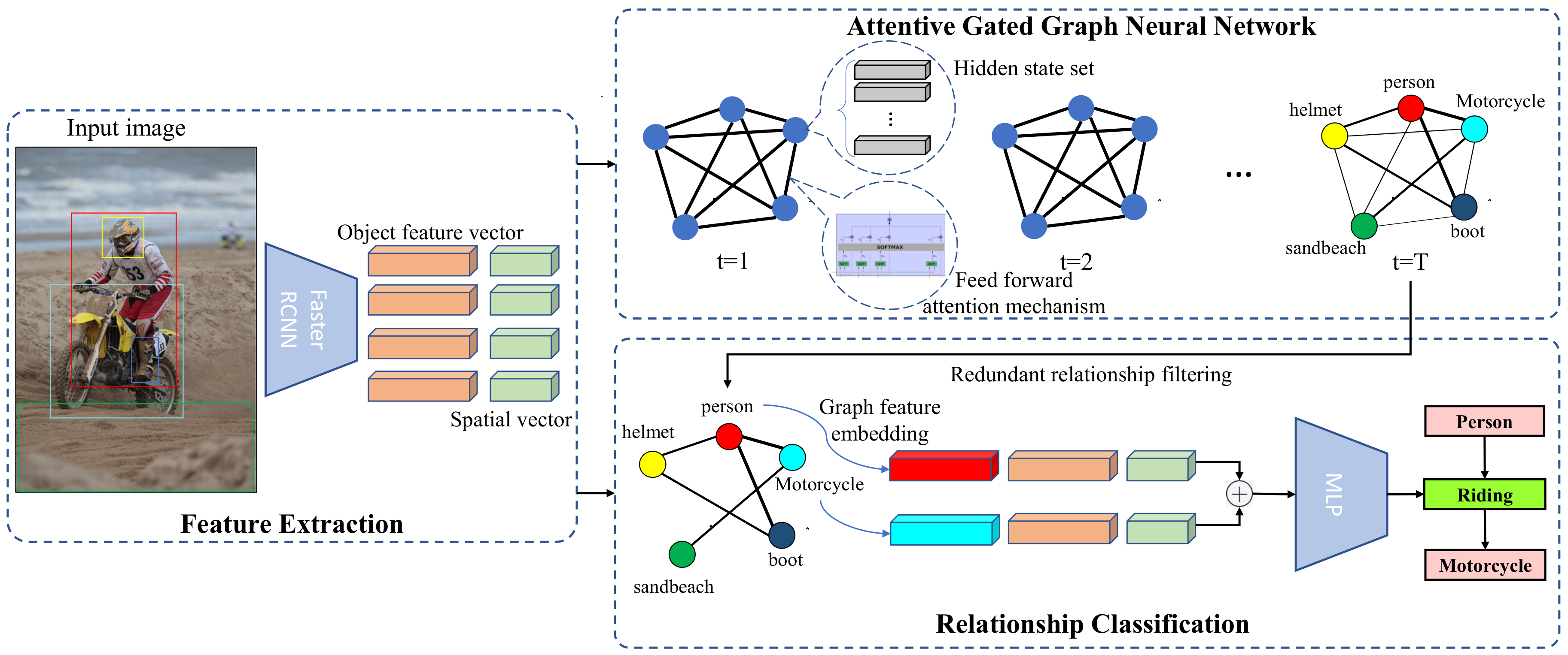
3. Methodology

We define the scene graph of an image I as G, which consists of a set of object bounding boxes B, a set of corresponding class labels of bounding boxes O, and a set of relationships of all objects pairs R. Thus, we can define $G=〈B,O,R〉$, where $B=\left\{b_1,b_2,\cdots ,b_n\right\}$, $b_i\in {\mathbb{R}}^4$ denotes the bounding box for the i-th region, $O=\left\{o_1,o_2,\cdots ,o_n\right\}$, $o_i\in \left\{0,1,2,\cdots ,N_o\right\}$ denotes the class label of the i-th region, $N_o$ is the total number of object categories. $R=\left\{r_1,r_2,\cdots ,r_m\right\}$, $r_i$ is a triplet <S-P-O> format, where S is the subject, P is the predicate and O is the object. The triplet includes a subject node $\left(b_i,o_i\right)\in B\times O$, an object node $\left(b_i,o_i\right)\in B\times O$, and a relationship label $l_{i\to j}\in \left\{0,1,2,\cdots ,N_r\right\}$. $N_r$ is the total number of relationship categories between the given object pairs in dataset.

After the definition of the scene graph, the possibility of generating a scene graph from an image I can be composed by three components as similar to [28]:

$$P\left(G\mid I\right)=P\left(B\mid I\right)P\left(O\mid B,I\right)P\left(R\mid B,O,I\right).$$

(1)

This equation can be regarded as the factorization without independence assumptions. $P\left(B\mid I\right)$ represents the possibility of bounding boxes generating from input image, which can be inferred by the object detection module. $P\left(O\mid B,I\right)$ represents the possibility of object classification based on bounding box and input image. $P\left(R\mid B,O,I\right)$ represents the possibility of relationship classification based on object classification, bounding boxes, and input image.

Figure 2 illustrates an overall pipeline of our proposed method, which contains three modules, namely feature extraction module, attention gated graph neural network module, and relationship classification module. Feature extraction modules can be regarded as $P\left(B\mid I\right)$, which is implemented by the widely used Faster R-CNN [1]. Attention gated graph neural network module can be regarded as $P\left(O\mid B,I\right)$. We adopt a graph LSTMs with feed forward attention mechanism to classify object in bounding box. Relationship classification module can be regarded as $P\left(R\mid B,O,I\right)$. We integrate multiple features like embedded graph feature, object feature, and spatial feature and use a Multilayer Perception (MLP) to classify relationship based on the fused feature.

3.1. Feature Extraction

In our method, we employ Faster R-CNN to generate the set of bounding boxes. Spatial vectors $B=\left\{b_1,b_2,\cdots ,b_n\right\}$ which contain the spatial information of objects can be obtained by region proposal network in Faster R-CNN. Object feature vectors $F=\left\{f_1,f_2,\cdots ,f_n\right\}$ which contain the semantic information of objects can be obtained by Region Of Interest (ROI) pooling layer. These two types of feature vectors will be fed into AGGNN and relationship classification modules.

3.2. Attentive Gated Graph Neural Network

Intuitively, individual predictions of objects and relationships can benefit from their surrounding context. Inspired by the recent development of graph neural network [31,32], we introduce an attentive gated graph neural network which is implemented by graph LSTMs for scene graph modeling to classify object and sparse relationships. In this network, the message propagates on the connections between neuron units. With continuous recurring on temporal dimension, the graph network will have the ability to learn contextualized representation to predict the class label of each neuron node and discard the redundant connections.

First of all, we should define some variables. We count the statistical co-occurrence probabilities of objects from different categories on the training dataset, which we used in this paper is Visual Genome [12]. For example, for two categories ’person’ and ’boot’, we count the probability $m_{{}^{\prime }perso{n}^{\prime \prime }boo{t}^{\prime }}$ of the existence of object belonging to the category ’person’ and another object belonging to the category ’boot’. Let us assume that the number of the categories is C. We count these co-occurrence probabilities for all object pair and obtain a matrix $M_C\in {\mathbb{R}}^{C\times C}$, where $m_{c{c}^{{}^{\prime }}}\in M_C$. Then, we correlate the bounding boxes from B based on $M_C$. Because the category of the region in bounding box is unknown, it may belong to any one of the categories in dataset. So we duplicate node $b_i$C times to obtain a set of subnodes $\left\{b_{i,1},b_{i,2},\cdots ,b_{i,C}\right\}$, where subnode $b_{i,c}$ denotes the correlation of the region in bounding box $b_i$. Thus, $m_{c{c}^{{}^{\prime }}}$ is the correlation between $b_{i,c}$ and $b_{j,c^{{}^{\prime }}}$.

As the special sequence model which can encode irregular graph data, graph LSTMs have shown superior performance on tasks such as semantic object parsing. The core of the LSTMs is that every unit has a memory-cell and three gates which control the propagation of message. When we use graph LSTMs to model scene graph, each LSTMs unit corresponds to the object node in scene graph. Intuitively, node $b_i$ which contains a set of subnodes can be regarded as LSTMs unit. At timestep t, each subnode $b_{i,c}$ has a hidden state ${\mathbf{h}}_{i,c}^t$. As each subnode corresponds to the same region in bounding box $b_i$, we use object feature vector $f_i$ and box vector $b_i$ to initialize the hidden state at timestep 0. The equation can be formulated as

$${\mathbf{h}}_{i,c}^0={\varphi }_a\left(〈f_i,b_i〉\right),$$

(2)

where ${\varphi }_a$ is a fully connected layer which transform high-dimensional vector into low-dimensional vector. $〈,〉$ represents the concat computation. We assume that ${\mathbf{a}}_{i,c}^t$ is the input of the subnode $b_{i,c}$. Then, the subnode take ${\mathbf{a}}_{i,c}^t$ and its previous state as input to update its hidden state by cell and gated mechanisms. The functions are defined as follows:

$$\begin{array}{cc}\hfill {\mathbf{I}}_{i,c}^t& =\sigma \left({\mathbf{W}}_a^I{\mathbf{a}}_{i,c}^t+{\mathbf{U}}_a^I{\mathbf{h}}_{i,c}^{t-1}+{\mathbf{b}}_I\right),\hfill \\ \hfill {\mathbf{F}}_{i,c}^t& =\sigma \left({\mathbf{W}}_a^F{\mathbf{a}}_{i,c}^t+{\mathbf{U}}_a^F{\mathbf{h}}_{i,c}^{t-1}+{\mathbf{b}}_F\right),\hfill \\ \hfill {\mathbf{O}}_{i,c}^t& =\sigma \left({\mathbf{W}}_a^O{\mathbf{a}}_{i,c}^t+{\mathbf{U}}_a^O{\mathbf{h}}_{i,c}^{t-1}+{\mathbf{b}}_O\right),\hfill \\ \hfill {\mathbf{G}}_{i,c}^t& =tanh\left({\mathbf{W}}_a^G{\mathbf{a}}_{i,c}^t+{\mathbf{U}}_a^G{\mathbf{h}}_{i,c}^{t-1}+{\mathbf{b}}_G\right),\hfill \\ \hfill {\mathbf{C}}_{i,c}^t& ={\mathbf{F}}_{i,c}^t\odot {\mathbf{C}}_{i,c}^{t-1}+{\mathbf{I}}_{i,c}^t\odot {\mathbf{G}}_{i,c}^{t-1},\hfill \\ \hfill {\mathbf{h}}_{i,c}^t& ={\mathbf{O}}_{i,c}^t\odot tanh\left({\mathbf{C}}_{i,c}^t\right),\hfill \end{array}$$

(3)

where ${\mathbf{I}}_{i,c}^t$, ${\mathbf{F}}_{i,c}^t$, and ${\mathbf{O}}_{i,c}^t$ represent input gate, forget gate, and output gate respectively. ⊙ represents the element-wise product. Memory-cell ${\mathbf{C}}_{i,c}^t$ encodes the information of previous memory-cell ${\mathbf{C}}_{i,c}^{t-1}$ and current input. ${\mathbf{W}}_a^{*}$ and ${\mathbf{U}}_a^{*}$ are the embedding parameters which map the feature vector to the same space as LSTMs unit. ${\mathbf{b}}_{*}$ is the bias term.

At each timestep t, each subnode aggregates message from its neighbors according to the graph structure. The input of the subnode ${\mathbf{a}}_{i,c}^t$ can be obtained by feed forward attention mechanism based on the hidden state of the others nodes and can be formulated as

$$a_{i,c}^t=〈\sum _{j=1,j\ne i}^n{\alpha }_{ji}^{\to }\sum _{c^{{}^{\prime }}=1}^C{m}_{c^{{}^{\prime }}c}{\mathbf{h}}_{j,c^{{}^{\prime }}}^{t-1},\sum _{j=1,j\ne i}^n{\alpha }_{ij}^{\to }\sum _{c^{{}^{\prime }}=1}^C{m}_{c{c}^{{}^{\prime }}}{\mathbf{h}}_{j,c^{{}^{\prime }}}^{t-1}〉,$$

(4)

where ${\sum }_{j=1,j\ne i}^n{\alpha }_{ji}^{\to }=1$ and ${\sum }_{j=1,j\ne i}^n{\alpha }_{ij}^{\to }=1$, ${\alpha }_{ji}^{\to }and{\alpha }_{ij}^{\to }\in {\mathbf{A}}^{\to }$. ${\alpha }_{ji}^{\to }=1$ is the attention coefficient when $b_{i,c}$ is the subject, and ${\alpha }_j^{\to }$ is the attention coefficient when $b_{i,c}$ is the object. n is the number of all nodes in graph.

To emphasize, we update the attention coefficients of node $b_i$ by the following equation:

$$\begin{array}{cc}\hfill {\mathbf{e}}_i^{\to }& ={\mathbf{w}}^{T}tanh\left({\mathbf{W}}_A\sum _{c=1}^C\left[{\mathbf{h}}_{i,c}^{t-1}*\sum _{c^{{}^{\prime }}=1}^C{m}_{c^{{}^{\prime }}c}\right]+{\mathbf{b}}_A\right),\hfill \\ \hfill {\alpha }_{ji}^{\to }& =\frac{exp\left(e_{ji}^{\to }\right)}{{\sum }_{j=1,j\ne i}^{n}exp\left(e_{ji}^{\to }\right)},\hfill \end{array}$$

(5)

where $e_{ji}^{\to }\in {\mathbf{e}}_i$, ${\mathbf{W}}_A$, ${\mathbf{w}}^T$ are trainable weights of attention mechanism, and ${\mathbf{b}}_A$ is the bias term. In the process of model training, we note that ${\mathbf{W}}_A$ has a variable dimension with the number of nodes in scene graph. We set this dimension as a fixed value N. When the scene graph has n nodes in the training or inferring stage, the first n dimensions parameters of ${\mathbf{W}}_A$ are used. ${\alpha }_{ij}^{\to }$ can be obtained by computing the attention coefficients of node $b_j$. At timestep t, we compute the attention coefficients of all nodes in graph. Thus, the input $a_{*}^t$ for each subnode can be obtained.

In this way, each node can aggregate messages from the other nodes and transfer its message to the other nodes in the meantime, enabling interactions among all nodes in the graph. After T timesteps, we can obtain the final hidden state for each node, which can be represented by a set of subnode $\left\{{\mathbf{h}}_{i,1}^T,{\mathbf{h}}_{i,2}^T,\cdots ,{\mathbf{h}}_{i,C}^T\right\}$. Similar to [28], we use a fully connected layer that takes the initial hidden state and final hidden state as input to compute the output feature for each subnode

$${\mathbf{f}}_{i,c}={\varphi }_b\left(〈{\mathbf{h}}_{i,c}^0,{\mathbf{h}}_{i,c}^0.〉\right)$$

(6)

Finally, we aggregate all correlated output feature vectors of subnodes to predict the class label of node, formulated as

$${\mathbf{o}}_i={\varphi }_c\left(\sum _{c=1}^C{\mathbf{f}}_{i,c}\right),$$

(7)

where ${\varphi }_c$ is a fully connected layer.

Then the class label of node will be obtained by SoftMax layer

$$l_i=softmax\left({\mathbf{o}}_i\right),$$

(8)

where $l_i$ is the predicted class label of node $b_i$.

3.3. Relationship Classification

After the T-th iterations of the attentive gated LSTMs, we will obtain the convergent attention coefficients ${\mathbf{A}}^{\to }$. There are two connections ${\alpha }_{ij}^{\to }$ and ${\alpha }_{ji}^{\to }$ for each node pair $b_i$ and $b_j$. However, there is only one directional connection between node pair in scene graph. We define the attentive score $s_{ij}$ between object pair as

$$p_{ij}^a=max\left({\alpha }_{ii}^{\to },{\alpha }_{ji}^{\to }\right).$$

(9)

Thus, a slightly sparse scene graph with $C_n^2$ connections can be obtained. However, not all nodes have connections in practice. To reduce the computational complexity of relationship classification module, we need to prune unlikely scene graph connections further.

To this, we count the probabilities of all possible relationships given a subject of the category c and an object of the category $c^{{}^{\prime }}$, which is denoted as statistical score $p_{(i=c,j=c^{{}^{\prime }})}^s$. We define relatedness score $p_{ij}$ as

$$p_{ij}={\omega }_1*p_{ij}^a+{\omega }_2*p_{(i=c,j=c^{{}^{\prime }})}^s,$$

(10)

where ${\omega }_1$ and ${\omega }_2$ are hyper-parameters to tune the function, and ${\omega }_1+{\omega }_2=1$. Then, a sparse post-pruning scene graph are obtained by setting threshold for relatedness score.

Our model attempts to explore the structural information to classify the relationship between nodes. The embedding graph feature of node $b_i$ can be represented as follows:

$${\mathbf{emb}}_i=\sum _{i=1}^C{\mathbf{h}}_{i,c}^T.$$

(11)

Then, we perform classification of relationship between node $b_i$ and $b_j$ with CNN as follows:

$$l_{i,j}=CNN\left(\left[\begin{array}{c}〈{\mathbf{emb}}_i,f_i,b_i〉\\ 〈{\mathbf{emb}}_j,f_j,b_j〉\end{array}\right]\right),$$

(12)

where $l_{i,j}$ refer to the predicted label of relationship. We adopt two cross-entropy loss function in the training stage, and define $l_i^{*}$ and $l_{i,j}^{*}$ as the ground-truth label for object and relationship, respectively:

$$\begin{array}{cc}\hfill {\mathit{L}}_{object}& =-\sum _i{l}_{i}log\left(l_i^{*}\right),\hfill \\ \hfill {\mathit{L}}_{relationship}& =-\sum _i\sum _{j\ne i}{l}_{i,j}log\left(l_{i,j}^{*}\right).\hfill \end{array}$$

(13)

We define the joint objective loss function in our model as follows:

$$\mathit{L}={\lambda }_1*{\mathit{L}}_{object}+{\lambda }_2*{\mathit{L}}_{relationship}+{∥\mathbb{W}∥}_2^2,$$

(14)

where ${\lambda }_1$ and ${\lambda }_2$ denote hyper-parameters, and $\mathbb{W}$ refers to all trainable weights in our model.

4. Results

In this section, we present a detailed evaluation of our model. Extensive experiments are conducted on the popular Visual Genome dataset [12].

4.1. Dataset and Implementation Details

Dataset We evaluate the proposed method and comparing methods on the popular Visual Genome (VG) dataset. The Original VG dataset contains 108,077 images with an average of 38 objects and 22 relationships per image. It is a challenging and widely used benchmark for scene graph generation. However, a substantial fraction of the object annotations has poor-quality and overlapping bounding boxes and/or ambiguous object names. We manually cleaned up the original dataset following previous work [13]. The new dataset contains an average of 25 distinct objects and 22 relationships per image. we used the most frequent 150 object categories and 50 predicates for evaluation. We called this dataset which had been cleaned up as clean VG (CVG). However, there are still many inaccuracies in the cleaned annotations. For examples, it is not sure if the category of wheel in skateboard is “wheel” or “wheels”, the relationship between “person” and “skirt” is “wears” or “wearing”, and the relationship between “cat” and “eyes” is “has” or “of”. In our experiment, we further unified these words so that different words could express the same meaning. More specifically, we used gerund instead of verb if they appeared in the dataset at the same time, the singular and plural forms of a noun, whichever is more, will be used, and “has”, ”on”, and “of”, whichever is more in an image, will be used. After that, we used the most frequent 150 object categories and 50 predicates for evaluation. We called this dataset as deep clean VG (DCVG). Both CVG and DCVG are divided into the training set and test set by 70%, 30%, respectively. We further picked 5000 images from training set as the validation set for hyper-parameter tuning.

Implementation Details We implement our model based on TensorFlow [33] framework on the NVIDIA 2080 Ti GPU. Similar to prior works for scene graph generation [13,28,29], we adopt Faster R-CNN detector (with VGG16 pretrained in ImageNet dataset) [1] as backbone in feature extraction module. During training, the number of proposals from RPN is 256. For each proposal, we perform ROI pooling to get a $7\times 7$ feature map, and a two-layer MLP encode the feature map to a feature vector with 1024-d. First, we finetune the Faster R-CNN using SGD algorithm with initial learning rate of $1\times {10}^{-4}$, batch size 16, momentum of 0.9, and weight decay of $1\times {10}^{-4}$. After that, we perform an end-to-end training by employing Adam as the optimizer with initial learning rate of $1\times {10}^{-6}$ for Faster R-CNN, $1\times {10}^{-4}$ for the other networks, and the exponential decay rates for momentums are set as 0.9 and 0.999. We adopt a mini-batch training with batch size 8 and weight decay as $1\times {10}^{-4}$. The hyper-parameters in Equation (10) are set as ${\omega }_1:{\omega }_2=4:6$, and the hyper-parameters in Equation (14) are set as ${\lambda }_1:{\lambda }_2=7:3$. Furthermore, the size of spatial vector is 4, the size of hidden state vector in grated LSTMs is 512. The CNN in Equation (12) is composed of one convolutional layer, one max-pooling layer, and two fully connected layers. There has 16 kernels in convolutional layer which size is $2\times 2$, the kernel of max-pooling layer is $1\times 2$, the first fully connected layer outputs a vector of size 500, and the second layer outputs a vector of size 51.

4.2. Evaluation Metrics and Tasks

Evaluation Metrics. Following [28,29], Top-K Recall (denoted as Rec@K ) is used to evaluate how many labelled relationships are hit in the Top-K predictions. The reason we use Recall instead of mean Average Precision (mAP) is that annotations of the relationships are not complete. Ref. [26] has detailed discussion to this problem. In our experiments, Recall@100 and Recall@50 are our evaluation metrics.

Tasks. Our aim to generate the scene graph for image, the key points are relationship classification and graph generation, while we no longer evaluate the accuracy of object detection. Predicate Classification (PredCls): Given the original images and a set of ground-truth entity bounding boxes with their corresponding localization and categories, the goal is to predict all relations between objects. Scene Graph Classification (SGCls): Given the original images and a set of ground-truth entity bounding boxes only with their corresponding localization, the goal is to predict the category of all objects and relations in an image. This task needs to correctly detect the triplet of <subject-predicate-object>. Similar to [13], scene graph generation needs to localize both the subject and the object with at least 0.5 IOU (intersection over union) in our evaluation.

4.3. Quantitative Comparisons

We compare our model with the existing state-of-the-art methods on Original VG dataset, CVG dataset, and DCVG dataset: Visual Relationship Detection (VRD) [12], Multi-level Scene Description Network (MSDN) [14], they are the early methods which implement their methods on Original VG; Iterative Message Passing (IMP) [13] and its improved version by using a better detector (IMP+) [4], Motif Network(MotifNet) [4], Graph R-CNN [3], Knowledge-Embedded Routing Network (KERN) [28], Graph-Permutation Invariant (GPI), Attentive Relational Networks (ARN) [29], they basically followed the data prepossessing method in [13]. In all experiments, the parameter settings of the above-mentioned methods are adopted from the corresponding papers.

We report the scene graph generation performance in

Table 1. Comparison results of our model and existing state-of-the-art methods on predicate classification (PredCls) task and scene graph classification (SGCls) task on the test sets of Original VG, CVG, and DCVG. Ours w/o att+emb, Ours w/ att, Ours w/ emb and Ours full denote our model without attention mechanism and graph feature embedding, our model only with attention mechanism, our model only with graph feature embedding and our full model, respectively. The best results are in bold and italic.

Dataset	Models	PredCls		SGCls		Mean
		Recall@50	Recall@100	Recall@50	Recall@100
Original VG	VRD [12]	27.9	35.0	11.8	14.1	22.2
	MSDN [14]	56.0	61.0	25.8	27.8	42.7
CVG	IMP [13]	44.8	53.0	21.7	24.4	36.0
	IMP+ [4]	59.3	61.3	34.6	35.4	47.6
	MotifNet [4]	65.2	67.1	35.8	36.5	51.1
	Graph R-CNN [3]	54.2	59.1	28.5	35.9	44.4
	KERN [28]	65.8	67.6	36.7	37.4	51.9
	GPI [34]	65.1	66.9	36.5	38.8	51.8
	ARN [29]	56.6	61.3	38.2	40.4	49.1
	Ours w/o att+emb	57.3	59.8	31.7	33.8	45.7
	Ours w/ att	63.5	65.9	35.4	37.1	50.5
	Ours w/ emb	59.1	61.8	33.6	35.3	47.4
	Ours full	65.1	67.2	36.8	38.2	51.8
DCVG	Ours w/o att+emb	58.6	61.3	33.9	35.8	47.4
	Ours w/ att	65.3	67.2	37.2	38.5	52.0
	Ours w/ emb	60.7	63.2	36.3	37.7	49.5
	Ours full	66.2	68.3	38.5	40.1	53.3

. As shown in this table, our proposed model (Ours full) has the comparable results with the other previous models on CVG dataset. In the case that the best results on CVG dataset are distributed in different methods, our method ranks second in three metrics, and the other index ranks the third place. Although many scene graph models are evaluated on different versions of Visual Genome, the mean recall of ours full model is the comparable. Our method also achieves a better effect on DCVG dataset, in which different representations of a category have been unified.

Ablations To evaluate the effectiveness of our main model, we consider several ablations in Table 1. In our w/o att+emb model, we predict objects based on feature extraction module, graph LSTMs, and relationship classification without graph feature embedding, and it is the baseline of our model. We find that it has reached a better level compared to previous methods. In our w/ att model, feed forward attention mechanism is applied in gated graph LSTMs, but graph feature embedding is not used. The results show that it has a great improvement compared with baseline, which fully shows the role of attention mechanism. In Our w/ att model, fully connected LSTMs are used to encode the scene graph, embed graph feature is used to classify relationship. The results show that structural feature is playing an important part in relationship classification. When both attention mechanism and graph feature embedding are used in our model, our model works best.

4.4. Qualitative Results

Figure 3 shows generated scene graphs for test set images from DCVG dataset with attentive gated graph LSTMs for SGCls task. There are two common failure cases of our model. First, as exhibited in Figure 3a, “a man is holding a frisbee” is mistakenly identified as “a man is throwing a frisbee”. However, the meaning of “holding” and “throwing” is similar meaning in this figure. Secondly, our model is not clear enough about the logical expression of objects in complex scenes. For examples, in Figure 3b, the relationship between “table” and “water” is mistakenly classified. Nevertheless, our model is able to generate scene graphs with high quality in most scenarios.

5. Conclusions

This paper proposed a novel end-to-end neural network system that could automatically generate a scene graph of an image. Our method consists of three modules: feature extraction, attentive gated graph neural network and relationship classification. The gated graph neural network is applied to encode the fully connected scene graph and propagate message between objects. The feed forward attention mechanism is integrated into graph network to prune the redundancy connections and enhance the accuracy of classification. Through extensive ablation experiments, we demonstrate that gated graph network and attention mechanism improve the effect of image scene graph generation to a certain extent, respectively. In addition, our method has the comparable results with the state-of-the-arts for scene graph generation, as evaluated by widely used metrics.

References

- Ren, S.; He, K.; Girshick, R.; Sun, J. Faster r-cnn: Towards real-time object detection with region proposal networks. In Advances in Neural Information Processing Systems; MIT Press: Cambridge, MA, USA, 2015; pp. 91–99. [Google Scholar]
- Redmon, J.; Divvala, S.; Girshick, R.; Farhadi, A. You only look once: Unified, real-time object detection. In Proceedings of the IEEE Conference on Computer Vision and Pattern Recognition, Las Vegas, NV, USA, 27–30 June 2016; pp. 779–788. [Google Scholar]
- Yang, J.; Lu, J.; Lee, S.; Batra, D.; Parikh, D. Graph r-cnn for scene graph generation. In Proceedings of the European Conference on Computer Vision (ECCV), Munich, Germany, 8–14 September 2018; pp. 670–685. [Google Scholar]
- Zellers, R.; Yatskar, M.; Thomson, S.; Choi, Y. Neural motifs: Scene graph parsing with global context. In Proceedings of the IEEE Conference on Computer Vision and Pattern Recognition, Las Vegas, NV, USA, 27–30 June 2016; pp. 5831–5840. [Google Scholar]
- Li, Y.; Ouyang, W.; Wang, X.; Tang, X. Vip-cnn: Visual phrase guided convolutional neural network. In Proceedings of the IEEE Conference on Computer Vision and Pattern Recognition, Honolulu, HI, USA, 21–26 July 2017; pp. 1347–1356. [Google Scholar]
- Klawonn, M.; Heim, E. Generating triples with adversarial networks for scene graph construction. In Proceedings of the Thirty-Second AAAI Conference on Artificial Intelligence, New Orleans, LA, USA, 2–7 February 2018. [Google Scholar]
- Johnson, J.; Krishna, R.; Stark, M.; Li, L.J.; Shamma, D.; Bernstein, M.; Fei-Fei, L. Image retrieval using scene graphs. In Proceedings of the IEEE Conference on Computer Vision and Pattern Recognition, Boston, MA, USA, 7–12 June 2015; pp. 3668–3678. [Google Scholar]
- Yao, T.; Pan, Y.; Li, Y.; Mei, T. Exploring visual relationship for image captioning. In Proceedings of the European Conference on Computer Vision (ECCV), Munich, Germany, 8–14 September 2018; pp. 684–699. [Google Scholar]
- Li, X.; Jiang, S. Know more say less: Image captioning based on scene graphs. IEEE Trans. Multimed. 2019, 21, 2117–2130. [Google Scholar] [CrossRef]
- Johnson, J.; Gupta, A.; Fei-Fei, L. Image generation from scene graphs. In Proceedings of the IEEE Conference on Computer Vision and Pattern Recognition, Salt Lake City, UT, USA, 18–22 June 2018; pp. 1219–1228. [Google Scholar]
- Teney, D.; Liu, L.; van Den Hengel, A. Graph-structured representations for visual question answering. In Proceedings of the IEEE Conference on Computer Vision and Pattern Recognition, Honolulu, HI, USA, 21–26 July 2017; pp. 1–9. [Google Scholar]
- Krishna, R.; Zhu, Y.; Groth, O.; Johnson, J.; Hata, K.; Kravitz, J.; Chen, S.; Kalantidis, Y.; Li, L.J.; Shamma, D.A.; et al. Visual genome: Connecting language and vision using crowdsourced dense image annotations. Int. J. Comput. Vis. 2017, 123, 32–73. [Google Scholar] [CrossRef]
- Xu, D.; Zhu, Y.; Choy, C.B.; Fei-Fei, L. Scene graph generation by iterative message passing. In Proceedings of the IEEE Conference on Computer Vision and Pattern Recognition, Honolulu, HI, USA, 21–26 July 2017; pp. 5410–5419. [Google Scholar]
- Li, Y.; Ouyang, W.; Zhou, B.; Wang, K.; Wang, X. Scene graph generation from objects, phrases and region captions. In Proceedings of the IEEE International Conference on Computer Vision, Venice, Italy, 22–29 October 2017; pp. 1261–1270. [Google Scholar]
- Galleguillos, C.; Rabinovich, A.; Belongie, S. Object categorization using co-occurrence, location and appearance. In Proceedings of the 2008 IEEE Conference on Computer Vision and Pattern Recognition, Anchorage, AK, USA, 23–28 June 2008; pp. 1–8. [Google Scholar]
- Dai, B.; Zhang, Y.; Lin, D. Detecting visual relationships with deep relational networks. In Proceedings of the IEEE Conference on Computer Vision and Pattern Recognition, Honolulu, HI, USA, 21–26 July 2017; pp. 3076–3086. [Google Scholar]
- Gkioxari, G.; Girshick, R.; Malik, J. Contextual action recognition with r* cnn. In Proceedings of the IEEE International Conference on Computer Vision, Santiago, Chile, 7–13 December 2015; pp. 1080–1088. [Google Scholar]
- Lu, C.; Krishna, R.; Bernstein, M.; Fei-Fei, L. Visual Relationship Detection with Language Priors. In Proceedings of the European Conference on Computer Vision, Amsterdam, The Netherlands, 11–14 October 2016; pp. 852–869. [Google Scholar]
- Plummer, B.A.; Mallya, A.; Cervantes, C.M.; Hockenmaier, J.; Lazebnik, S. Phrase localization and visual relationship detection with comprehensive image-language cues. In Proceedings of the IEEE International Conference on Computer Vision, Venice, Italy, 22–29 October 2017; pp. 1928–1937. [Google Scholar]
- Ben-Younes, H.; Cadene, R.; Thome, N.; Cord, M. Block: Bilinear superdiagonal fusion for visual question answering and visual relationship detection. In Proceedings of the AAAI Conference on Artificial Intelligence, Honolulu, HI, USA, 27 January–1 February 2019; Volume 33, pp. 8102–8109. [Google Scholar]
- Xu, K.; Ba, J.; Kiros, R.; Cho, K.; Courville, A.; Salakhudinov, R.; Zemel, R.; Bengio, Y. Show, attend and tell: Neural image caption generation with visual attention. In Proceedings of the International Conference on Machine Learning, Lille, France, 6–11 July 2015; pp. 2048–2057. [Google Scholar]
- Wang, L.; Schwing, A.; Lazebnik, S. Diverse and accurate image description using a variational auto-encoder with an additive gaussian encoding space. In Advances in Neural Information Processing Systems; MIT Press: Cambridge, MA, USA, 2017; pp. 5756–5766. [Google Scholar]
- Chen, C.; Mu, S.; Xiao, W.; Ye, Z.; Wu, L.; Ju, Q. Improving image captioning with conditional generative adversarial nets. In Proceedings of the AAAI Conference on Artificial Intelligence, Honolulu, HI, USA, 27 January–1 February 2019; Volume 33, pp. 8142–8150. [Google Scholar]
- Divvala, S.K.; Farhadi, A.; Guestrin, C. Learning everything about anything: Webly-supervised visual concept learning. In Proceedings of the IEEE Conference on Computer Vision and Pattern Recognition, Columbus, OH, USA, 23–28 June 2014; pp. 3270–3277. [Google Scholar]
- Yu, R.; Li, A.; Morariu, V.I.; Davis, L.S. Visual relationship detection with internal and external linguistic knowledge distillation. In Proceedings of the IEEE International Conference on Computer Vision, Venice, Italy, 22–29 October 2017; pp. 1974–1982. [Google Scholar]
- Li, Y.; Ouyang, W.; Zhou, B.; Shi, J.; Zhang, C.; Wang, X. Factorizable net: An efficient subgraph-based framework for scene graph generation. In Proceedings of the European Conference on Computer Vision (ECCV), Munich, Germany, 8–14 September 2018; pp. 335–351. [Google Scholar]
- Woo, S.; Kim, D.; Cho, D.; Kweon, I.S. Linknet: Relational embedding for scene graph. In Advances in Neural Information Processing Systems; MIT Press: Cambridge, MA, USA, 2018; pp. 560–570. [Google Scholar]
- Chen, T.; Yu, W.; Chen, R.; Lin, L. Knowledge-embedded routing network for scene graph generation. In Proceedings of the IEEE Conference on Computer Vision and Pattern Recognition, Cardiff, UK, 9–12 September 2019; pp. 6163–6171. [Google Scholar]
- Qi, M.; Li, W.; Yang, Z.; Wang, Y.; Luo, J. Attentive relational networks for mapping images to scene graphs. In Proceedings of the IEEE Conference on Computer Vision and Pattern Recognition, Cardiff, UK, 9–12 September 2019; pp. 3957–3966. [Google Scholar]
- Vaswani, A.; Shazeer, N.; Parmar, N.; Uszkoreit, J.; Jones, L.; Gomez, A.N.; Kaiser, L.; Polosukhin, I. Attention is all you need. In Advances in Neural Information Processing Systems; MIT Press: Cambridge, MA, USA, 2017; pp. 5998–6008. [Google Scholar]
- Liang, X.; Shen, X.; Feng, J.; Lin, L.; Yan, S. Semantic object parsing with graph lstm. In Proceedings of the European Conference on Computer Vision, Amsterdam, The Netherlands, 11–14 October 2016; pp. 125–143. [Google Scholar]
- Wu, Z.; Pan, S.; Chen, F.; Long, G.; Zhang, C.; Yu, P.S. A comprehensive survey on graph neural networks. arXiv 2019, arXiv:1901.00596. [Google Scholar] [CrossRef] [PubMed]
- Abadi, M.; Barham, P.; Chen, J.; Chen, Z.; Davis, A.; Dean, J.; Devin, M.; Ghemawat, S.; Irving, G.; Isard, M.; et al. Tensorflow: A system for large-scale machine learning. In Proceedings of the 12th USENIX Symposium on Operating Systems Design and Implementation (OSDI 16), Savannah, GA, USA, 2–4 November 2016; pp. 265–283. [Google Scholar]
- Herzig, R.; Raboh, M.; Chechik, G.; Berant, J.; Globerson, A. Mapping images to scene graphs with permutation-invariant structured prediction. In Advances in Neural Information Processing Systems; MIT Press: Cambridge, MA, USA, 2018; pp. 7211–7221. [Google Scholar]