Article

Metric Factorization with Item Cooccurrence for Recommendation

College of Information Science and Engineering, Xinjiang University, Urumqi 830046, China
*
Author to whom correspondence should be addressed.
Symmetry 2020, 12(4), 512; https://doi.org/10.3390/sym12040512
Submission received: 12 February 2020 / Revised: 17 March 2020 / Accepted: 18 March 2020 / Published: 2 April 2020

Abstract

:
In modern recommender systems, matrix factorization has been widely used to decompose the user–item matrix into user and item latent factors. However, the inner product in matrix factorization does not satisfy the triangle inequality, and the problem of sparse data is also encountered. In this paper, we propose a novel recommendation model, namely, metric factorization with item cooccurrence for recommendation (MFIC), which uses the Euclidean distance to jointly decompose the user–item interaction matrix and the item–item cooccurrence with shared latent factors. The item cooccurrence matrix is obtained from the colike matrix through the calculation of pointwise mutual information. The main contributions of this paper are as follows: (1) The MFIC model is not only suitable for rating prediction and item ranking, but can also well overcome the problem of sparse data. (2) This model incorporates the item cooccurrence matrix into metric learning so it can better learn the spatial positions of users and items. (3) Extensive experiments on a number of real-world datasets show that the proposed method substantially outperforms the compared algorithm in both rating prediction and item ranking.

1. Introduction

In the era of information overload, recommendation systems are important for addressing the problem of information explosion. Collaborative filtering technology is an early, widely used, and influential recommendation technology, but its performance is severely degraded by data sparseness [1,2,3]. In the past decade, the factorization of user–item matrices into user and item latent factor vectors has been widely studied and has become a popular method for matrix factorization models. Furthermore, it not only has high prediction accuracy but can also well integrate and decompose additional side information. However, its performance will be affected by the choice of the inner product [4,5,6] because the inner product in matrix factorization does not satisfy the triangle inequality: “the distance between two points cannot be larger than the sum of their distances from a third point” [7]. This will limit the expressive power of the matrix factorization and lead to locally optimal solution problems, thereby reducing the flexibility and generalization performance of the matrix factorization model. The metric learning method of the Euclidean distance is more suitable for the learning of latent factors [8,9,10]. Metric factorization is based on the learning of user–item factors based on the Euclidean distance. It is important to encode the user–item interaction matrix for the construction of a distance matrix that is suitable for the learning of the Euclidean distance. Although metric learning has overcome the shortcomings of matrix factorization, in the case of sparse data, learning only the latent factors of users and items remains insufficient. Therefore, we propose the metric factorization with item cooccurrence model, in which the item cooccurrence matrix is introduced into the metric learning process so that the user–item interaction matrix and the item–item cooccurrence matrix with shared item latent factors can be decomposed simultaneously during metric learning. The key strategy for item cooccurrence is to construct a colike item matrix. The value that corresponds to each pair of items is the number of users who have called the colike matrix coding, and the item cooccurrence matrix contains the calculated pointwise mutual information values of the colike item matrix.
Our main contributions are as follows. (1) We propose a new recommendation model: metric factorization with item cooccurrence (MFIC). We designated two variants of MFIC to solve two classic and well-established recommendation tasks: rating prediction and item ranking, and they can overcome the problem of sparsity data. (2) The user–item interaction matrix and the introduced item occurrence matrix learn together in metric space, which is more conducive to better learning the spatial positions of users and items. (3) Extensive experiments on a number of real-world datasets demonstrate that our model outperforms the compared algorithm in terms of both rating estimation and item ranking tasks.
The remaining sections of this paper are organized as follows. Section 2 describes the related work; Section 3 shows the MFIC model; Section 4 presents the experimental results and analysis; and Section 5 summarizes the paper.

2. Related Works

2.1. Matrix Factorization

In recommendation systems, matrix factorization is a popular and effective recommendation method and is the standard in modern recommendation systems. The successful implementation of many potential factor models is based on matrix factorization. The most basic matrix factorization strategy is to decompose the rating matrix into latent factors of users and items. By learning to establish the relationship between users and items, the accuracy of recommendation prediction is improved [11,12]. With the development of recommendation systems, many variants of matrix factorization have been derived, and user and item bias terms have been introduced to improve the prediction accuracy of the model [13]. A graph probability model was introduced to better adapt to the real data sparse environment [14,15]. The authors in [16] proposed a novel quality of service prediction approach based on probabilistic matrix factorization, which has the capability of incorporating network location and implicit associations among users and services. Mature algorithms also utilize SVD ++ [17] and timeSVD [18]. Another special processing method is to push the unobserved user–item pairs away from the observed user–item pairs from the Bayesian perspective to solve the problem of item ranking [19].

2.2. Item Embedding

The item cooccurrence matrix that was developed in this paper was inspired by the word embedding model. In the word embedding model, each word is represented by a real vector [20]. Word2vec is a popular word embedding method. For a specified series of training words, its embedding model learns the potential factors of each word. For example, in [21], the surrounding words of a specified word are predicted during training. The study by [22] also used the word embedding model to build item embedding models for learning prediction, and [23] introduced item embedding into the matrix factorization model, and the performance was substantially improved. Reference [24] added not only user and item embeddings, but also items that users do not like into the matrix factorization model for prediction, and the accuracy of the prediction was also improved. Therefore, we introduced item cooccurrence in this paper, and we processed the user–item matrix to construct the item cooccurrence matrix, which better facilitates metric learning.

3. Metric Factorization with Item Cooccurrence (MFIC) Model

First, we reviewed two basic frameworks for creating MFIC models: metric factorization for recommendation beyond matrix factorization (FML) and word embedding. Then, we describe how our MFIC model and calculus are calculated.

3.1. Factorized Metric Learning (FML )Model

The FML model is a model for metric learning that uses the Euclidean distance. First, the user rating matrix   R R m × n is transformed into a distance matrix R 1 R 1 m × n , the distance matrix is obtained via Equation (1).
D i s t a n c e ( u , i ) = M a x   S i m i l a r i t y S i m i l a r i t y ( u , i )
Max Similarity is the maximum value of the rating matrix (e.g., 5) or implicit feedback (e.g., 1).
In the metric vector space, we denote the positions of users and items as P u R k and Q i R k , respectively. The main optimization loss functions of FML are as follows.
L ( P , Q ) = c u i   ( Y u i Y ^ ) 2
Y ^ 1 = | | P Q | | 2 2 + b u + b i + μ
Y ^ 2 = | | P Q | | 2 2
In rating prediction, Equation (3) was selected as the prediction distance, where b u and b i represent user and item biases, respectively, while μ represents global biases. Super-parameter τ is added in front of μ to scale and obtain a more accurate prediction value. c u i is a self-confidence mechanism for ensuring that extreme ratings are assigned higher self-confidence values. Equation (4) was selected as the predictive distance when ranking items. c u i is the self-confidence mechanism of the observed items.

3.2. Word Embedding

The word embedding model has realized substantial success in natural language processing and has received increasing attention. Word embedding is a generalization of language modeling and representation learning technology in natural language processing that mainly maps all the dimensions into the high latitude of each word or phrase of the real field vector that is embedded into a low-dimensional vector space. In the popular word2vec [20], a set of words are specified and each word is embedded from a high-dimensional domain vector into a low-dimensional vector space. Finally, the skip-gram model in word2vec is used to predict the words around it in a fixed window. For example, as shown in Figure 1, we selected the word “my” as the input word, and set skip_window = 2, where skip_window = 2 represents selecting the left two words and the right two words of the input word “my” to enter our window, and obtain the training data of four groups.
According to [25,26], the skip-gram model with negative sampling is equivalent to implicit factorization of a word context matrix in which entry is the pointwise mutual information (PMI) of the corresponding word and context, which is shifted by a global constant. Let D be the set of observed words and context pairs. The PMI between word i and its word context j is calculated as
P M I ( i , j ) = l o g ( ( P ( i , j ) / ( P ( i ) P ( j ) ) ) )                        
P ( i , j ) = # ( i , j ) / | D |                        
P ( i ) = # ( i ) / | D |                      
P ( j ) = # ( j ) / | D |                          
where # ( ) represents the frequency of words, for example, # ( i , j ) represents the frequency of the simultaneous occurrence of the words i and j in order to calculate the probability P ( i , j ) of the two. P ( i , j ) denotes the probability that word i and word j appears simultaneously in a fixed window, P ( i ) represents the probability of occurrence of word i in set D, and P ( j ) is the probability of word j appearing alone in set D. Substituting Equations (6)–(8) into Equation (5) yields the following expression (9):
P M I ( i , j ) = l o g ( ( # ( i , j ) | D | ) / ( # ( i ) # ( j ) ) )                  
PMI can be constructed as a matrix of size m × n , namely, matrix MPMI, where m is the number of elements in set D. Next, the shifted positive pointwise mutual information (SPPMI) of words i and j is calculated as:
S P P M I ( i , j ) = m a x ( P M I ( i , j ) l o g ( k ) , 0 )
Here, k is a hyperparameter, which can control the matrix density of the PMI and has an inverse proportional relationship, namely, the larger the value of k, the higher the sparsity of matrix PMI. The main advantage is that optimization adjustments are unnecessary. The above is the complete process of word embedding.

3.3. MFIC Model

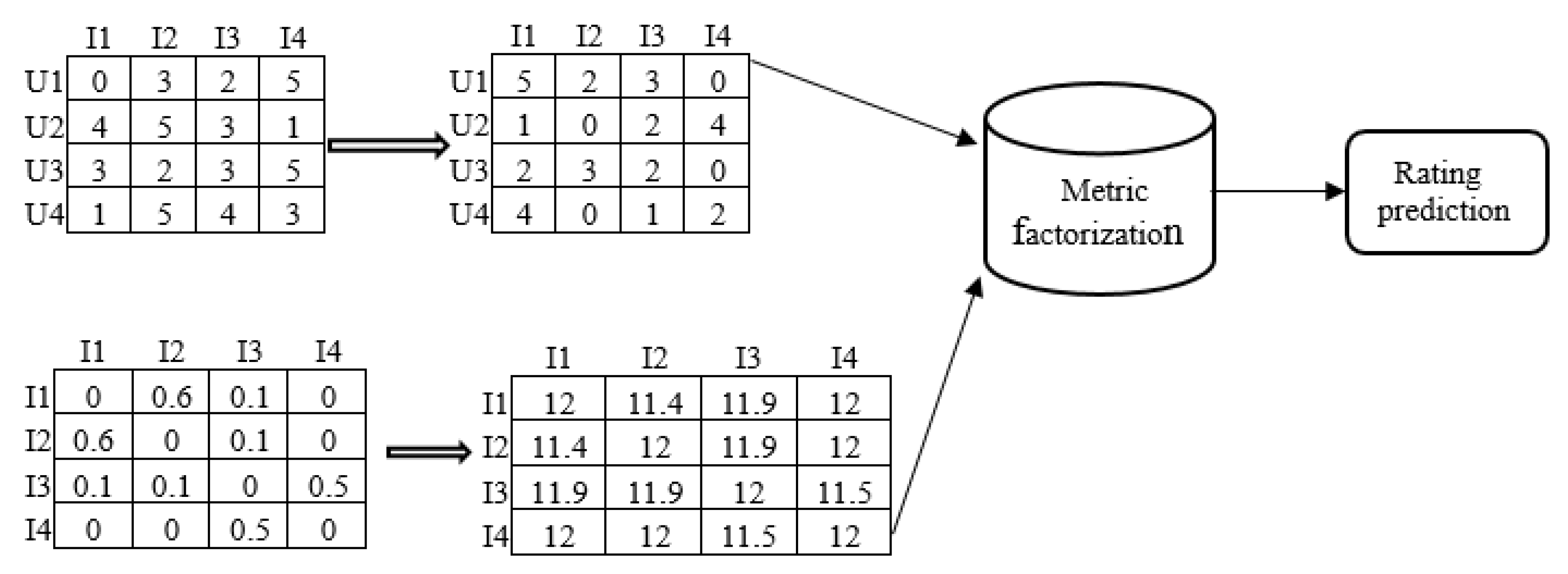
Inspired by word embedding, the colike item matrix is created via word embedding. We can think of the items called by the user as the words in the word embedding, therefore, we can create the colike item matrix according to word embedding and use it to identify the item latent factors. In addition, this colike item matrix is symmetrical about the diagonal of the matrix. As illustrated in Figure 2, I1 and I2 are called by U1, U3, and U4 in the user–item matrix simultaneously; therefore, the corresponding value of item1 and item2 in the colike matrix is 3. I1 and I4 have not been called by any same user. Hence, the corresponding value is empty. This matrix was generated and merged with metric learning in this paper. The rating matrix was calculated and used to find the item that is called by each user, which is equivalent to using # ( i ) and # ( j )   in word embedding to search for the item that is consumed by the corresponding two users, which is equivalent to word embedding # ( i , j ) . Before constructing the item cooccurrence SPPMI matrix, the mutual information of each pair of points must be calculated via Equation (5). Then, the shifted positive pointwise mutual information of item–item pairs is calculated via Equation (10) from the obtained pointwise mutual information. According to the colike item matrix in Figure 2, # ( I 1 , I 2 ) = 3 , #(I1 = 3), and # ( I 2 ) = 2 , | D | = 8 , and after calculation, the mutual information value of I1 and I2 is 0.60, as presented in the item embedding matrix of Figure 3. Finally, it is embedded into the metric learning model to highlight the item’s expressiveness and to enhance the relationships between users and items and between items and items.
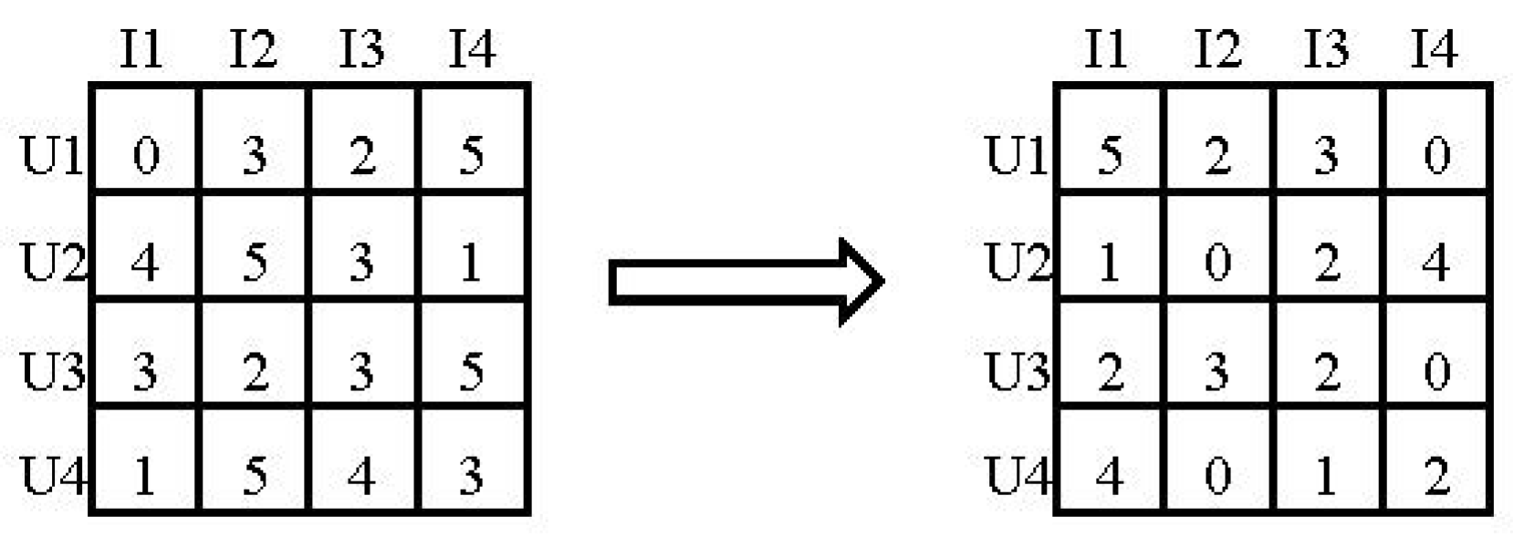
To use the metric vector space to learn user and item positions via factorization, it is necessary to convert the user rating matrix into a distance matrix to improve the learning in the metric space. The distance matrix can be constructed from the explicit distance matrix and the implicit distance matrix. A checkmark in the explicit matrix indicates that the user has invoked the item, and a cross sign indicates that the item has not been invoked. The transformation of the explicit distance matrix obeys the following transformation rule.
D i s t a n c e ( u , i ) = M a x   S i m i l a r i t y S i m i l a r i t y ( u , i )            
where Max Similarity is the maximum value in the rating matrix such as five.
The transformation of the implicit distance matrix satisfies the following equality.
D i s t a n c e ( u , i ) = β ( 1 S i m i l a r i t y ( u , i ) )
In the implicit case, the Similarity(u,i) is 1 or 0, while parameter β in the formula is used to control the balance between the user and the item. Figure 4 and Figure 5 present schematic transformations of the explicit preference matrix and the implicit preference matrix.

3.4. Evaluation for Rating Prediction

The MFIC model combines metric factorization and item cooccurrence and simultaneously performs the position learning of the latent factors of users and items in the metric space. The difference between metric factorization and item cooccurrence is that metric factorization infers the form for encoding a user’s preference for an item, whereas an item embedding must be interpreted from the item cooccurrence model. The overall model of the MFIC rating prediction is illustrated in Figure 3.
L = ( 1 α ) c u i ( Y u i Y 1 ) 2 + α c u i ( Y u i Y 2 ) 2 +   λ ( | | P u | | + | | Q i | | + | | Q i 1 | | )
D ( u , i ) = | | P u Q i | | 2
Y 1 = ( 1 γ ) D ( u , i ) + γ D ( i 1 , i ) + b u + b i + μ
Y 2 = D ( i 1 , i ) + b i 1
c u i = 1 + θ g ( R u i R m a x )
Equation (13) is the objective function of the MFIC model, and α is used as the weight coefficient for weighting the Y1 and Y2 losses so that the model finds the optimal value faster during loss learning. The last term in the equation is the regularization term, λ is the regularization term parameter, and | | P u | | , | | Q i | | , and | | Q i 1 | | are set to | | P u | | < c , | | Q i | | < c , and | | Q i 1 | | < c , which can control the | | P u | | , | | Q i | | , and | | Q i 1 | | unit spheres, respectively, in the L2-norm to spread the data points less widely and to facilitate multidimensional complexity treatment. Equation (14) expresses a learning method for the spatial positions of users and items that use the Euclidean distance in the metric space. In the metric vector space, we denote the positions of the user and the item as P u R k and Q i R k . Equation (15) represents the predicted value of the rating that is generated by the user and the item and by the item and the embedded item, and it enhances the connection between the user and the item. γ is a hyperparameter for controlling the balance between the user and the item, and the item and the embedded item. In matrix factorization [13], some items are popular and easily obtain high ratings, while some users habitually assign low ratings to items. Therefore, similar to matrix factorization, biases are added to metric learning to improve the stability and expressiveness of the model.   b u and b i represent the user bias and the item bias, respectively. μ is a global bias, which can be multiplied by a hyperparameter to improve the performance of the model. Equation (16) predicts the newly added item embedding. The prediction between the item and the embedded item can highlight the performance of the item, and b i 1 is the bias of the embedded item. Equation (17) is a self-confidence mechanism that assigns a high degree of self-confidence to extreme ratings [27]. g(*) can be an absolute value function, a square function, or a logarithmic function. It can be selected according to the requirements of the model. θ is a scaling parameter of the self-confidence mechanism that is used to control the degree of self-confidence in rating.

3.5. Evaluation for Ranking Prediction

Similarly, the item cooccurrence is introduced into the item ranking model to improve the item ranking performance in the personalized recommendation system. In the process of personalized recommendation item ranking, implicit data processing outperforms explicit data prediction. In previous studies, binary processing is typically used for implicit data [28,29,30]. Therefore, the explicit data were also implicitly processed in this paper. For example, a rating that is greater than or equal to 3.5 will be represented as 1, and a rating that is less than 3.5 will be represented as 0. The setting of the rating threshold will be elaborated in the experimental part.
L = ( 1 α ) c u i ( Y u i Y 1 ) 2 + α c u i ( Y u i Y 2 ) 2 +   λ ( | | P u | | + | | Q i | | + | | Q i 1 | | )
c u i = 1 + θ W u i
The use of Equation (18) is consistent with the prediction of the rating. The largest difference is that c u i in Equation (19) is different. c u i is still a self-confidence mechanism in item ranking, and θ is a scaling hyperparameter. W u i represents the number of times the user has responded to positive feedback regarding the item. For example, if the user calls the item three times, W u i = 3 . This is more conducive to users being closer to their favorite items and farther away from the items that they do not like. In addition, the embedding of the item not only highlights the item’s expressiveness, but also increases the connections between users and items.

3.6. Optimization and Prediction

Dropout was added into the MFIC model training. Dropout is an effective method in neural networks for dealing with the fitting process [31], therefore, this paper used dropout to prevent the overfitting of models in Euclidean distance learning for user and item latent factors. In addition, for the model loss function learning, a loss learning model, namely, Adagrad [32], was adopted, which can adapt the learning step size according to the update frequency of the model and reduce the frequency of parameter adjustment. Finally, because the rating matrix is converted from a distance matrix at the beginning of the model, the predicted distance matrix must be reversed for rating prediction, and for item ranking, the closeness of the item to the user depends on the predicted distance.

4. Experimental Evaluation

We studied the performances of the MFIC models in rating prediction and item ranking, and we used various datasets and evaluation indicators to measure and evaluate the performances of MFIC models in rating prediction and item ranking to determine the impacts of model parameters on the model performance, to compare the performances of MFIC models with those of other recommendation methods, and to analyze the experimental results.

4.1. Preparation for the Rating Prediction Experiments and Presentation of the Experimental Result

The datasets for rating prediction are Movielens-100K and Movielens-1M [27]. During the experiment, the datasets were randomly divided into training sets and test sets according to the ratio of 9:1. The sparsity is the number of existing ratings divided by the number of users and the number of items. Details on the datasets are presented in Table 1.
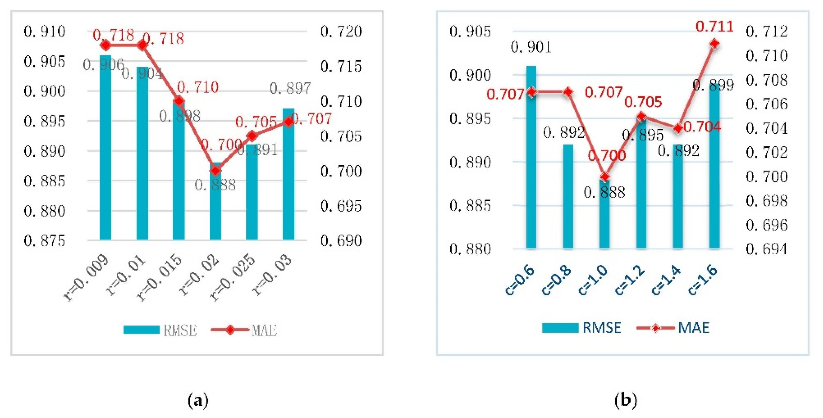
The selection of important parameters of the MFIC model has a substantial influence on the prediction performance. The training order of the parameters is r, c, N, τ, θ, d, γ, λ, α, s, and k. First, all parameters were set on the basis of the FML model27. Second, inspired by the parameter settings section in [33], one of the parameters was trained and a set of values was selected for iterative training. For example, on the dataset Movielens-100K, we tested the learning rate r of [0.009, 0.01, 0.015, 0.02, 0.025, 0.03], the different clip value c of [0.6, 0.8, 1.0, 1.2, 1.4, 1.6], and dimension N of [50, 100, 150, 200, 250, 300], the hyperparameter τ was tuned amongst [0.6, 0.7, 0.8, 0.9, 1.0, 1.1], the self-confidence value θ was tuned amongst [0, 0.1, 0.2, 0.3, 0.4, 0.5], the dropout rate d was tuned amongst [0.01, 0.03, 0.05, 0.07, 0.09, 0.11], the prediction function weight γ was performed in [0, 0.001, 0.002, 0.003, 0.004, 0.005], the regularization weight λ was performed in [0.001, 0.005, 0.01, 0.05, 0.1, 0.6], and the loss function weight α was performed in [0.001, 0.003, 0.005, 0.01, 0.03, 0.05]. Furthermore, the rating threshold s was selected from [0, 1, 2, 3, 4], and the pointwise mutual information value k was selected from [0, 1, 3, 5, 7, 9]. Finally, the next parameter was trained on the basis of the optimal parameters. For example, when the training parameter was c, the remaining parameters were fixed and r was set to the optimal value that had been trained. The stopping criterion is that the evaluation indicator root mean squared error (RMSE) was not further reduced. We obtained the optimal setting as follows: Movielens-100K (r = 0.02, c = 1.0, N = 150, τ = 0.8, θ = 0.2, d = 0.05, γ = 0.002, λ = 0.01, α = 0.01, s > 1, and k ≥ 1). In the same way, the optimal setting is as follows: Movielens-1M (r = 0.02, c = 1.4, N = 150, τ = 0.5, θ = 0.1, d = 0.03, γ = 0.002, λ = 0.01, α = 0.01, s > 3.5, and k ≥ 0.5). Figure 6 plots the effects of only the important parameters on the performance of the MFIC model during training on Movielens-100K.
Figure 6a presents the tuning of the learning rate to the model parameters. After continuous training, when the learning rate was r = 0.02, the predicted rating error was the smallest in terms of mean average error (MAE) or root mean squared error (RMSE). The clip value is a range of spatial positions that control the user and item latent factors. A suitable clip value can effectively address spatial multidimensional problems. According to Figure 6b, c = 1.0 is the most suitable. The number of dimensions N determines the number of latent vectors; too large a value will increase the complexity of the model, whereas too small a value will reduce the expressiveness of the features. Therefore, according to Figure 6c, when N = 150, the performance of the model is optimal. The parameter τ can be regarded as a scaling super-parameter of the global bias term that enables the model to find the accurate prediction value. From Figure 6d, it can be concluded that the super-parameter τ facilitates the improvement of the model performance and the prediction error was reduced when τ = 0.8. Figure 6e shows that when θ = 0.2, the rating prediction error was the smallest. When θ = 0, the performance of the model was drastically reduced. The confidence value θ is indispensable in this model. Dropout was utilized to prevent latent user and item factors from being overfit during training. According to Figure 6f, the value that was selected by the dropout rate was too large or too small to help the model. Therefore, d = 0.05 was selected. The weight loss of the prediction function was used to balance the contributions of users and items, and items and embedded items to the rating prediction (see Equation (14)). Figure 6g shows that γ = 0.002 was the best choice for the model. The regularization term λ was added to prevent overfitting of the model. According to Figure 6h, λ = 0.01 should be set. Inspired by [34], this paper also added the loss function weight α to the model to control each loss function term. According to Figure 6i, α = 0.01 should be selected.
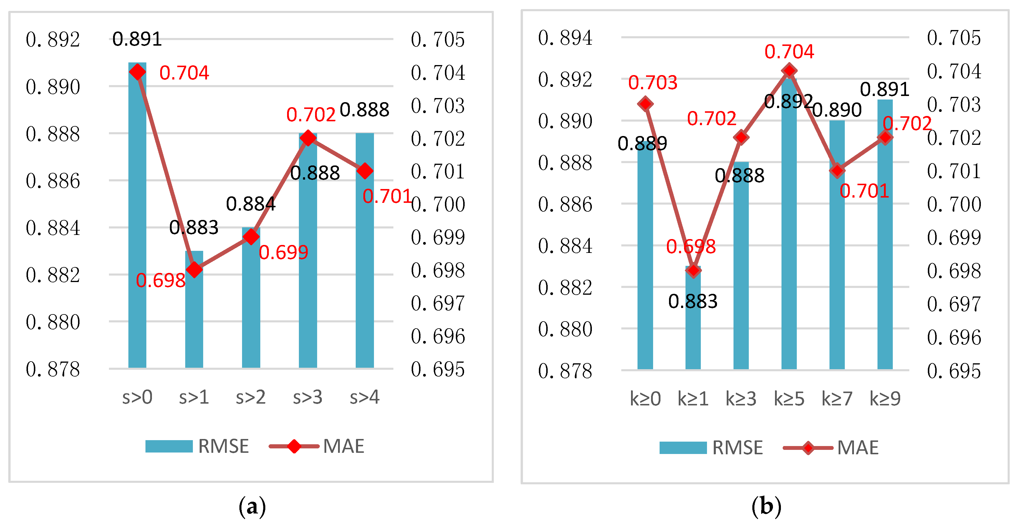
The rating threshold s was used to select data when constructing the item cooccurrence matrix such as s > 1, which caused all ratings that exceeded 1 in the dataset to be selected, namely, only the data with ratings of 2, 3, 4, and 5 were selected for item cooccurrence. In the construction of the matrix, the ratings that have little effect on the model are removed, and the complexity of the model is reduced. Figure 7a shows that when the selection rating threshold satisfies s > 1, the error of the rating prediction was the smallest and the error of the previous rating prediction was reduced. The pointwise mutual information value was calculated according to Equation (8). According to Equation (9), k is the setting choice of the pointwise mutual information value in the item cooccurrence matrix; for example, if k ≥ 3, the culling pointwise mutual information value is in the range of 0 ≤ k < 3, and the model complexity can be reduced again. According to Figure 7b, a pointwise mutual information value that satisfies k ≥ 3 should be selected.
To make the experimental results more accurate and representative, this paper used two evaluation indicators (MAE and RMSE) in the rating prediction, conducted six evaluations for each comparison method, and averaged the results. To evaluate the performance of MFIC in rating prediction, this paper considered the following comparison algorithms: bayesian probabilistic matrix factorization (BPMF) is a probabilistic matrix factorization model with a full Bayesian processing method that uses the Markov chain Monte Carlo method to train the model [15]. Neural rating regression (NRR) is a prediction rating model that is based on the deep learning framework neural rating tips (NRT) [35]. Neural network matrix factorization (NNMF) uses a multilayer neural network to change the inner product of matrix factorization to realize rating prediction [36]. FML uses the Euclidean distance instead of the inner product of matrix factorization for metric space learning and rating prediction.
It can be concluded from Table 2 that the MFIC model outperformed all the comparison algorithms in rating prediction and realized satisfactory prediction performance on datasets Movielens-1M and Movielens-100K, which differ in terms of density. In addition, from the data in Table 2, it can be seen that the evaluation indicators MAE and RMSE of the algorithm BPMF on the dataset Movielens-1M were better than the algorithm NRR, but in the dataset Movielens-100K, the opposite was true, and MFIC in these two dataset both of them have achieved good experimental results, indicating that the MFIC model can also show relatively stable performance on these two datasets with different densities. Thus, the introduction of item cooccurrence can improve the rating prediction performance.

4.2. Item Ranking Experiment Preparation and Experimental Results

The dataset that was used for item ranking was composed of two datasets, FilmTrust and EachMovie [27]. The dataset was divided into a training set and a test set according to the ratio of 8:2. Details on the dataset are presented in Table 3.
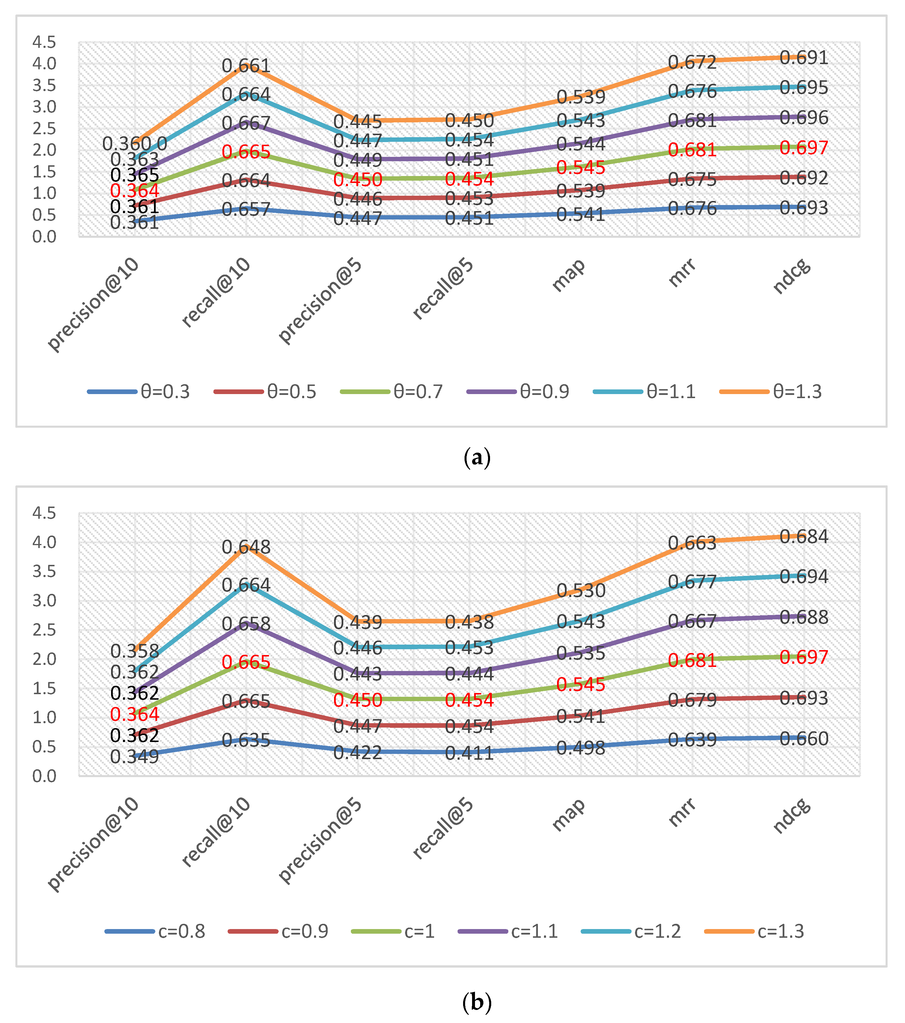
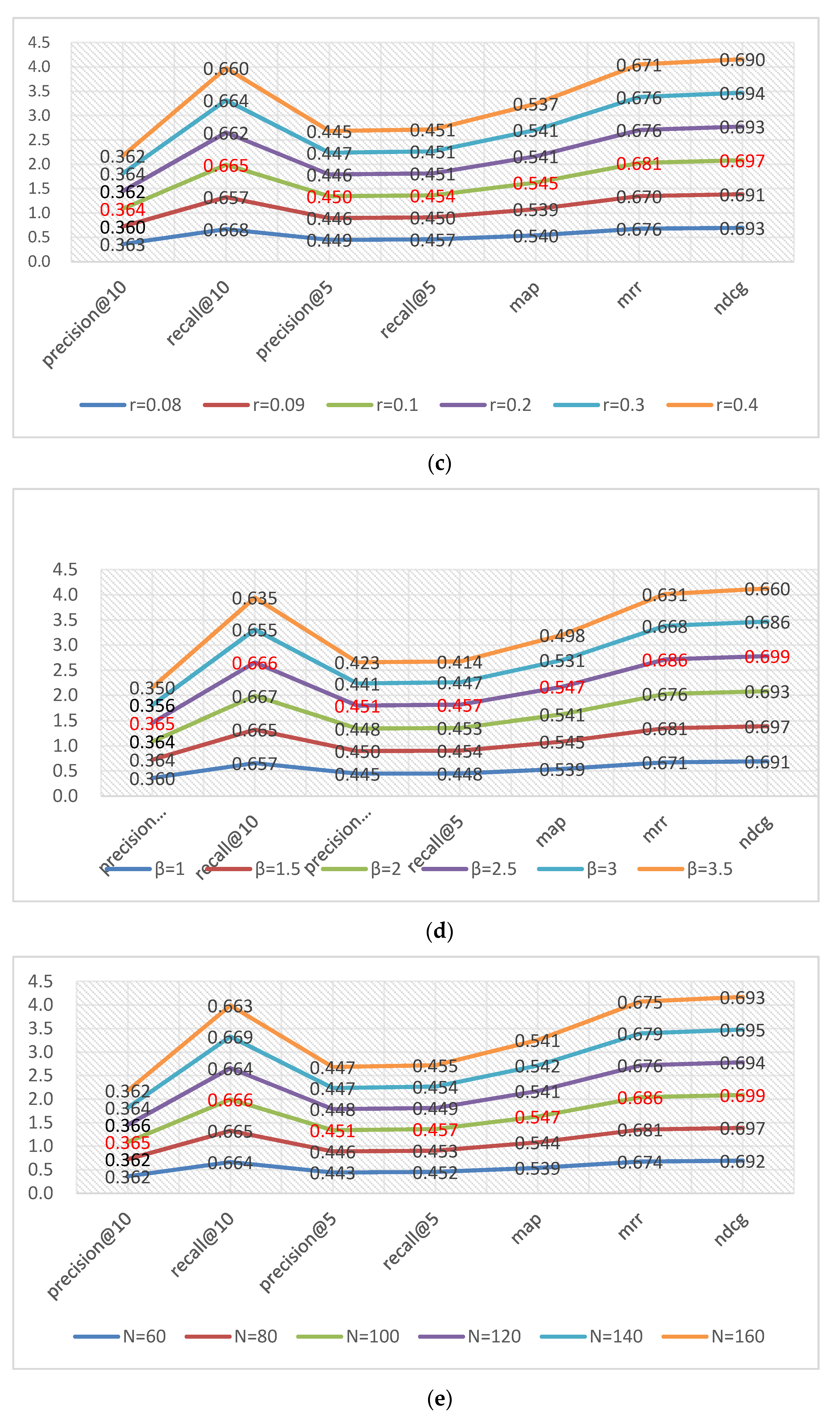
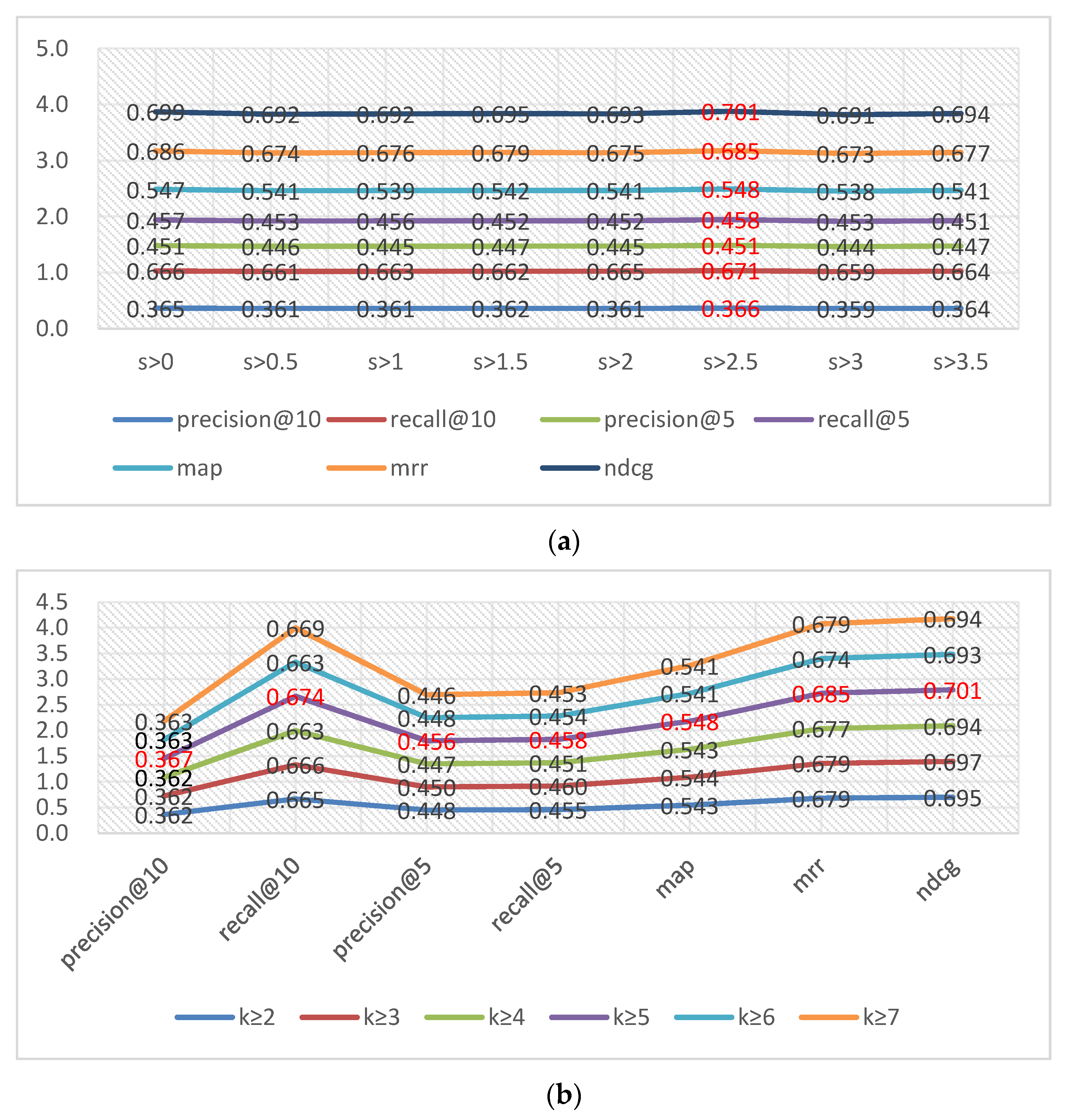
All parameters were tuned just like the rating prediction in Section 4.1, and we stopped training the model in the item ranking when the evaluation indicator Precision@5 showed no further improvement. We obtained the optimal setting as follows: FilmTrust (θ = 0.7, c = 1.0, r = 0.1, β = 2.5, N = 100, α = 0.01, d = 0.05, γ = 0.005, s > 2.5, and k ≥ 5) and EachMovie (θ = 0.1, c = 1.0, r = 0.1, β = 2, N = 100, α = 0.01, d = 0.05, γ = 0.005, s > 0.4, and k ≥ 0.4). The figure below shows the impacts of important parameters on FilmTrust on the performance of the MFIC model during training. Each line in the figure represents a parameter adjustment result. Each line in the figure is the result of this tuning. Each value on a line is an evaluation index. Additional details are presented in Figure 8. In Figure 9, the value that corresponds to each column in Figure 9a is the result of one round of tuning. Each value is an evaluation index, as shown in Figure 9b, as in Figure 8. Additional information is presented in Figure 9.
In Figure 8, the optimal values for each parameter were θ = 0.7, c = 1, r = 0.1, N = 100, α = 0.01, d = 0.05, and γ = 0.005. For hyperparameters θ, c, and r, the meanings of N, α, d, and γ were the same as in the rating prediction and will not be explained here. The distance scaling hyperparameter β is the minimum distance for which the control setting was negative for the user. As shown in Figure 8d, β = 2.5 was the optimal value for sorting the items.
The rating threshold s and the pointwise mutual information value k in Figure 9 were the same as those in the rating prediction and will not be explained here. As shown in Figure 9, when s > 2.5, the performance of the model was optimal. When k ≥ 5, the pointwise mutual information value was optimal for the model.
To accurately evaluate the item ranking performance of the MFIC model, this paper used several evaluation indicators such as the mean average precision (MAP), the mean reciprocal rank (MRR), the normalized discounted cumulative gain (NDCG), Recall@n, and Precision@n. The algorithm was trained six times and the average value was obtained to yield more representative experimental results. To evaluate the performance of the MFIC model, the following comparison algorithms were considered. The neural matrix factorization (NeuMF) model adopts a processing method in which a multilayer perceptron and matrix factorization are combined and used for item sequencing tests [4]. Collaborative denoising auto-encoders (CDAE) is a model with more flexible components that uses the strategy of automatic denoising encoders [37]. Weighted regularized matrix factorization (WRMF) is an item ranking test model with positive and negative preferences [2]. FML uses the Euclidean distance instead of the matrix decomposition inner product to learn the metric space and item rankings [27].
According to Table 4, the MFIC model also outperformed all comparison algorithms in item ranking, even on two datasets that differed in terms of density, namely, FilmTrust and EachMovie. Hence, MFIC can adapt to the environment of sparse data in the item ranking prediction. According to the experimental results, the metric learning used by MFIC far outperformed methods that use matrix factorization algorithms such as NeuMF and WRMF. In addition, the FML algorithm with metric learning can also be used for item ranking, but its prediction result was less accurate than the MFIC prediction result. Thus, the introduction of item cooccurrence can also substantially facilitate item ranking.

5. Conclusions

In this paper, we proposed a metric factorization method with item cooccurrence for recommendation, which mainly uses the word embedding strategy in natural language processing to conduct item cooccurrence and metric factorization learning in a recommendation system. First, the item cooccurrence matrix was constructed via the calculation of the pointwise mutual information value. Then, the user–item matrix and the item cooccurrence matrix were converted into the corresponding distance matrix, and the obtained distance matrix was decomposed into a metric space via the Euclidean distance for latent user, item, and embedded item factor spatial position learning. Finally, the performance in rating prediction and item ranking was evaluated. The experimental results on two datasets for rating prediction and item ranking show that the performance of the MFIC model has been substantially improved to that of other recommendation algorithms.

Author Contributions

Conceptualization, H.D. and L.W.; Methodology, H.D.; Software, H.D.; Validation, J.Q. and L.W.; Formal analysis, H.D.; Writing, original draft preparation, H.D.; Writing, review and editing, H.D.; Visualization, J.Q. All authors read and agreed to the published version of the manuscript.

Funding

The research was supported in part by the National Science Foundation of China (Grant Nos. 61867006 and 61771416); the Doctoral Scientific Research Foundation of Xinjiang University (Grant No. BS150263); the Education Reform Project of Higher Education of Xinjiang Uygur Autonomous Region named “A study on the application of teaching method combining mooc with flipping classroom.”; and the Higher Education Innovation Project of Xinjiang Uygur Autonomous Region (Grant No. XJEDU2017T002).

Conflicts of Interest

The authors declare no conflicts of interest.

References

  1. He, C.; Zhang, Q.; Tang, Y.; Liu, S.; Liu, H. Network Embedding Using Semi-Supervised Kernel Nonnegative Matrix Factorization. IEEE Access 2019, 7, 92732–92744. [Google Scholar] [CrossRef]
  2. Resnick, P.; Iacovou, N.; Suchak, M.; Bergstrom, P.; Riedl, J. GroupLens: An Open Architecture for Collaborative Filtering of Netnews. In Proceedings of the 1994 ACM conference on Computer Supported Cooperative Work, Chapel Hill, NC, USA, 22–26 October 1994; pp. 175–186. [Google Scholar]
  3. Su, X.; Khoshgoftaar, T.M. A Survey of Collaborative Filtering Techniques. In Advances in Artificial Intelligence; Hindawi LimitedAdam House: London, UK, 2009; Volume 2009, pp. 1–19. [Google Scholar]
  4. He, X.; Liao, L.; Zhang, H.; Nie, L.; Hu, X.; Chua, T.-S. Neural Collaborative Filtering. In Proceedings of the 26th International Conference on World Wide Web, Perth, Australia, 3–7 April 2017; pp. 173–182. [Google Scholar]
  5. Yue, S.; Larson, M.; Hanjalic, A. Collaborative Filtering beyond the User-Item Matrix: A Survey of the State of the Art and Future Challenges. ACM Comput. Surv. (CSUR) 2014, 47, 1–45. [Google Scholar]
  6. Ram, P.; Gray, A.G. Maximum inner-product search using cone trees. In Proceedings of the 18th ACM SIGKDD International Conference on Knowledge Discovery and Data Mining, Beijing, China, 12–16 August 2012; p. 931. [Google Scholar]
  7. Tversky, A.; Gati, I. Similarity, separability, and the triangle inequality. Psychol. Rev. 1982, 89, 123–154. [Google Scholar] [CrossRef] [PubMed]
  8. Hu, Y.; Koren, Y.; Volinsky, C. Collaborative Filtering for Implicit Feedback Datasets. In ICDM; IEEE Computer Society: Washington, DC, USA, 2008; pp. 263–272. [Google Scholar]
  9. Tay, Y.; Tuan, L.A.; Hui, S.C. Latent Relational Metric Learning via Memory-based Attention for Collaborative Ranking. In Proceedings of the Web Conference (WWW 2018), Lyon, France, 23–27 April 2018; pp. 729–739. [Google Scholar]
  10. Weinberger, K.Q.; Saul, L.K. Distance Metric Learning for Large Margin Nearest Neighbor Classification. J. Mach. Learn. Res. 2009, 10, 207–244. [Google Scholar]
  11. Hong, R.; Hu, Z.; Liu, L.; Wang, M.; Yan, S.; Tian, Q. Understanding Blooming Human Groups in Social Networks. IEEE Trans. Multimed. 2015, 17, 1980–1988. [Google Scholar] [CrossRef]
  12. Steck, H. Training and testing of recommender systems on data missing not at random. In Proceedings of the 16th ACM SIGKDD International Conference on Knowledge Discovery and Data Mining, Washington, DC, USA, 24–28 July 2010; pp. 713–722. [Google Scholar]
  13. Koren, Y.; Bell, R.; Volinsky, C. Matrix Factorization Techniques for Recommender Systems. Computer 2009, 42, 30–37. [Google Scholar] [CrossRef]
  14. Salakhutdinov, R. Probabilistic matrix factorization. In Proceedings of the 20th International Conference on Neural Information Processing Systems, Vancouver, BC, Canada, 3–6 December 2007; pp. 1257–1264. [Google Scholar]
  15. Salakhutdinov, R.; Mnih, A. Bayesian probabilistic matrix factorization using markov chain monte carlo. ICML 08. In Proceedings of the 25th International Conference on Machine Learning, Helsinki, Finland, 5–9 July 2008; pp. 880–887. [Google Scholar]
  16. Yin, Y.; Chen, L.; Xu, Y.; Wan, J. Location-Aware Service Recommendation With Enhanced Probabilistic Matrix Factorization. IEEE Access 2018, 6, 62815–62825. [Google Scholar] [CrossRef]
  17. Rubens, N.; Kaplan, D.; Sugiyama, M. Active learning in recommender systems. In Proceedings of the 19th International Conference on User Modeling, Adaption, Girona, Spain, 11–15 July 2011; pp. 414–417. [Google Scholar]
  18. Koren and Yehuda. Collaborative filtering with temporal dynamics. In Proceedings of the 15th ACM SIGKDD International Conference on Knowledge Discovery and Data Mining, Paris, France, 28 June–1 July 2009; pp. 447–456.
  19. Volkovs, M.; Yu, G.W. Effective Latent Models for Binary Feedback in Recommender Systems. In Proceedings of the 38th International ACM SIGIR Conference on Research and Development in Information Retrieval, Santiago, Chile, 9–13 August 2015; pp. 313–322. [Google Scholar]
  20. Levy, O.; Goldberg, Y. Neural Word Embedding as Implicit Matrix Factorization. In Proceedings of the 28th Conference on Neural Information Processing Systems (NIPS), Montreal, QC, Canada, 8–13 December 2014; pp. 2177–2185. [Google Scholar]
  21. Mikolov, T.; Sutskever, I.; Chen, K.; Corrado, G.; Dean, J. Distributed representations of words and phrases and their compositionality. NIPS’13. In Proceedings of the 26th International Conference on Neural Information Processing Systems, Lake Tahoe, NV, USA, 5–8 December 2013; pp. 3111–3119. [Google Scholar]
  22. Guardiasebaoun, E.; Guigue, V.; Gallinari, P. Latent Trajectory Modeling: A Light and Efficient Way to Introduce Time in Recommender Systems. In Proceedings of the 9th ACM Conference on Recommender Systems, Vienna, Austria, 16–20 September 2015; pp. 281–284. [Google Scholar]
  23. Liang, D.; Altosaar, J.; Charlin, L.; Blei, D.M. Factorization Meets the Item Embedding: Regularizing Matrix Factorization with Item Co-occurrence. In Proceedings of the 10th ACM Conference on Recommender Systems, Boston, MA, USA, 15–19 September 2016; pp. 59–66. [Google Scholar]
  24. Tran, T.; Lee, K.; Liao, Y.; Lee, D. Regularizing Matrix Factorization with User and Item Embeddings for Recommendation. In Proceedings of the 27th ACM International Conference on Information and Knowledge Managemen, Torino, Italy, 22–26 October 2018; pp. 687–696. [Google Scholar]
  25. He, X.; Zhang, H.; Kan, M.Y.; Chua, T.S. Fast Matrix Factorization for Online Recommendation with Implicit Feedback. In Proceedings of the 39th International ACM SIGIR conference on Research and Development in Information Retrieval, Pisa, Italy, 17–21 July 2016; pp. 549–558. [Google Scholar]
  26. Barkan, O.; Koenigstein, N. ITEM2VEC: Neural item embedding for collaborative filtering. In Proceedings of the 2016 IEEE 26th International Workshop on Machine Learning for Signal Processing (MLSP), Vietri sul Mare, Salerno, Italy, 13–16 September 2016; pp. 1–6. [Google Scholar]
  27. Shuai, Z.; Yao, L.; Yi, T.; Xu, X.; Zhu, L. Metric Factorization: Recommendation beyond Matrix Factorization. Comput. Sci. 2018, 6, 1–11. [Google Scholar]
  28. Koren, Y. Factorization meets the neighborhood: A multifaceted collaborative filtering model. In Proceedings of the 14th ACM SIGKDD International Conference on Knowledge Discovery and Data Mining, Las Vegas, NV, USA, 24–27 August 2008; pp. 426–434. [Google Scholar]
  29. Bayer, I.; He, X.; Kanagal, B.; Rendle, S. A generic coordinate descent framework for learning from implicit feedback. In Proceedings of the 26th International Conference on World Wide Web, Perth Australia, 3–7 April 2017; pp. 1341–1350. [Google Scholar]
  30. Liang, D.; Charlin, L.; Mcinerney, J.; Blei, D.M. Modeling User Exposure in Recommendation. WWW 16. In Proceedings of the 25th International Conference on World Wide Web, Montréal, QC, Canada, 11–15 May 2016; pp. 951–961. [Google Scholar]
  31. Srivastava, N.; Hinton, G.; Krizhevsky, A.; Sutskever, I.; Salakhutdinov, R. Dropout: A simple way to prevent neural networks from overfitting. J. Mach. Learn. Res. Arch. 2014, 15, 1929–1958. [Google Scholar]
  32. Duchi, J.; Hazan, E.; Singer, Y. Adaptive subgradient methods for online learning and stochastic optimization. J. Mach. Learn. Res. Arch. 2011, 12, 257–269. [Google Scholar]
  33. Tran, D.Q.V.; Tuan-Anh, N.P.; Gao, C. Attention-based Group Recommendation. Assoc. Comput. Mach. 2018, 1, 1–15. [Google Scholar]
  34. Hsieh, C.-K.; Yang, L.; Cui, Y.; Lin, T.-Y.; Belongie, S.; Estrin, D. Collaborative Metric Learning. In Proceedings of the 26th International Conference on World Wide Web (WWW ’17), Perth, Australia, 3–7 April 2017; pp. 193–201. [Google Scholar]
  35. Li, P.; Wang, Z.; Ren, Z.; Bing, L.; Lam, W. Neural rating regression with abstractive tips generation for recommendation, SIGIR’17. In Proceedings of the 40th International ACM SIGIR Conference on Research and Development in Information Retrieval, Tokyo, Japan, 7–11 August 2017; pp. 345–354. [Google Scholar]
  36. Dziugaite, G.K.; Roy, D.M. Neural Network Matrix Factorization. Comput. Sci. 2015, 11, 1–7. [Google Scholar]
  37. Wu, Y.; Dubois, C.; Zheng, A.X.; Ester, M. Collaborative Denoising Auto-Encoders for Top-N Recommender Systems, WSDM’16. In Proceedings of the Ninth ACM International Conference on Web Search and Data Mining, San Francisco, CA, USA, 22–25 February 2016; pp. 153–162. [Google Scholar]
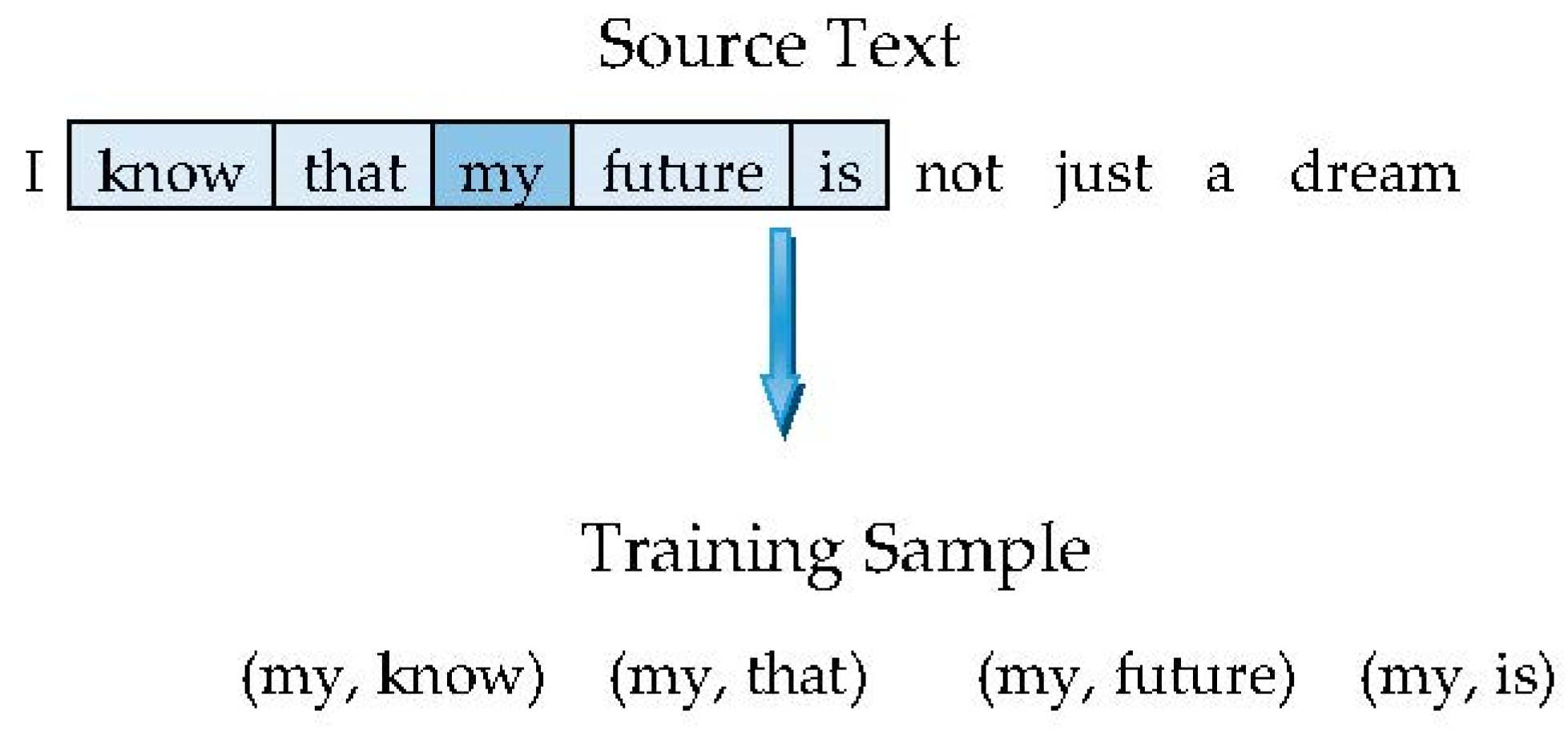
Figure 1. Getting word embedding through the skip-gram model.
Symmetry 12 00512 g001
Figure 2. Extracting an item in a user–item matrix where two items are simultaneously called by the same user to build a colike item matrix.
Symmetry 12 00512 g002
Figure 3. MFIC for the rating prediction model.
Symmetry 12 00512 g003
Figure 4. Converting a user’s explicit matrix to an explicit distance matrix according to Equation (11).
Symmetry 12 00512 g004
Figure 5. Converting the user’s implicit matrix to an implicit distance matrix according to Equation (12).
Symmetry 12 00512 g005
Figure 6. (a) The impact of the learning rate on the rating. (b) Clip value impact on the rating prediction performance. (c) The impact of the number of dimensions on the rating prediction performance. (d) The influence of hyperparameter τ on the rating prediction. (e) The impact of the confidence value on the rating prediction performance. (f) The impact of the dropout rate on the rating prediction performance. (g) The effect of the prediction function weights on rating prediction. (h) The effect of regularization on the rating prediction. (i) The influence of the loss function weight on the rating prediction.
Symmetry 12 00512 g006aSymmetry 12 00512 g006b
Figure 7. (a) The impacts of scoring thresholds on the rating. (b) The effect of the point mutual information value on rating.
Symmetry 12 00512 g007
Figure 8. (a)The effect of the confidence value θ on the model performance. (b) The impact of the clip value on the model performance. (c) The impact of the learning rate r on the model performance. (d) The effect of the distance scaling factor β on the model performance. (e) The effect of the number of dimensions N on the model performance. (f) The influence of the loss function weight α on the model performance. (g) The impact of the dropout rate d on the model performance. (h) The effect of the prediction function weight on the model performance.
Symmetry 12 00512 g008aSymmetry 12 00512 g008bSymmetry 12 00512 g008c
Figure 9. (a) The impact of scoring threshold s on the model performance. (b) The effect of PMI value k on the model performance.
Symmetry 12 00512 g009
Table 1. Details of datasets Movielens-100K and Movielens-1M.
DatasetsNumber of UsersNumber of ItemsTotal RatingRange of RatingSparsity
Movielens-100K9431682100,0000–56.30%
Movielens-1M604039521,000,2090–54.19%
Table 2. Demonstration and comparison of the performance of the MFIC model and other recommendation methods in the evaluation the MAE and RMSE of indicators on the following two datasets.
ModelMovielens-1MMovielens-100K
MAERMSEMAERMSE
BPMF0.6780.8670.7250.927
NRR0.6910.8750.7170.909
NNMF0.6690.8430.7090.903
FML0.6580.8440.7060.900
MFIC0.6530.8340.6880.883
Ours vs. best0.0050.0100.0080.017
Table 3. Details of the datasets FilmTrust and EachMovie.
DatasetsNumber of UsersNumber of ItemsTotal RatingRange of RatingSparsity
FilmTrust1508207135,4970–51.13%
EachMovie2952016481,048,5750–12.15%
Table 4. Item ranking performances of the MFIC model and other recommendation methods on seven evaluation indicators and two datasets.
FilmTrust
ModelMAPMRRNDCGRecall@5Precision@5Recall@10Precision@10
NeuMF0.4830.6090.6460.3930.4130.6260.350
CDAE0.5230.6540.6780.4410.4360.6470.353
WRMF0.5160.6480.6630.4270.4330.6320.351
FML0.5430.6810.6960.4520.4500.6680.364
MFIC0.5480.6850.7010.4580.4560.6740.367
Ours vs. best0.0050.0040.0050.0060.0050.0060.003
EachMovie
ModelMAPMRRNDCGRecall@5Precision@5Recall@10Precision@10
NeuMF0.4140.6560.6570.3350.3780.4750.302
CDAE0.4320.6780.6730.3560.3940.4970.311
WRMF0.4330.6790.6700.3550.3970.4940.314
FML0.4660.7080.6940.3920.4190.5330.325
MFIC0.4870.7280.7130.3990.4460.5390.349
Ours vs. best0.0210.0200.0190.0070.0270.0060.024