Article

Parametric Model for Kitchen Product Based on Cubic T-Bézier Curves with Symmetry

1
School of Mechanical and Precision Instrument Engineering, Xi’an University of Technology, Xi’an 710048, China
2
School of Art and Design, Xi’an University of Technology, Xi’an 710054, China
*
Author to whom correspondence should be addressed.
Symmetry 2020, 12(4), 505; https://doi.org/10.3390/sym12040505
Submission received: 23 February 2020 / Revised: 10 March 2020 / Accepted: 16 March 2020 / Published: 1 April 2020

Abstract

:
The parametric method of product design is a pivotal and practical technique in computer-aided design and manufacturing (CAD/CAM) and used in many manufacturing sectors. In this paper, we presented a novel parametric method to design a kitchen product in the residential environment, a kitchen cabinet, by using cubic T-Bézier curves with constraints of geometric continuities. First, we introduced a class of cubic T-Bézier curves with two shape parameters and derived the G1 and G2 continuity conditions of the cubic T-Bézier curves. Then, we constructed shape-controlled complex contour curves of the kitchen cabinet by using closed composite cubic T-Bézier curves. The shapes of the contour curves can be adjusted intuitively and predictably by altering the values of the shape parameters. Finally, we studied shape optimization and representation of ellipses for the contour curves of the kitchen cabinet by finding optimal shape parameters and applicable control points respectively. The provided modeling examples showed that our method in this paper can improve the design and scheme adjustment effectively in the conceptual design stage of kitchen products.

1. Introduction

With the development of modern manufacturing technology and the sustainably growing needs of the users, the appearance of kitchen products is getting more and more attention. As monotonous designs cannot meet the diverse needs of users, more creative designs are highly valued by manufacturers as it directly affects the market sales and brand competitions [1]. The traditional design method mainly relies on the designer’s experience and subjective cognition, the entire process is long, tedious and inefficient and some kitchen products with profiled modeling are still difficult to design [2].
With the development of digital technology, computer-aided design and manufacturing (CAD/CAM) technology are constantly updated and improved. Curves are classic tools of computer-aided geometric design (CAGD) and basic geometric elements of CAD/CAM technology [3,4]. The parametric design method is used to construct the curve model of the kitchen product, which can quickly generate a series of designs by modifying the parameter values, thereby improving the design efficiency. Thus, achieving parametric design through a computer aided design system has become the priority of the CAD system developer and kitchen product enterprises.
The parametric design method based on the curve model combines the design with the data algorithms, therefore, it has obvious advantages compared to the traditional product design method [5,6]. In recent years, scholars have proposed a series of methods for the parameterization of product modeling design. Shajay claimed parametric design thinking is a computationally-augmented and solution-oriented design thinking and has been verified in architecture, interior and furniture design [7]. Kyung et al. [8] used a genetic algorithm with an empirically defined fitness function to generate optimal product appearances with car design similarities, and the design alternatives generated by the methodology could help the actual design process. Padmanabhan et al. [9] presented an effective method to determine the optimal blank shape by using the deformation behavior predicted by salient features of non-uniform rational B-splines (NURBS) surfaces. Wang [10] proposed a parametric design method of human bodies by the unorganized cloud points. Huang et al. [11] presented a parametric design method based on wireframe-assisted deep learning for human body modeling. Pérez-Arribas and Pérez- Fernández proposed a new B-spline-based parametric design methodology for propeller blades in [12]. In [13], Koini et al. designed an efficient NURBS-based software tool to accomplish the parametric design of turbomachinery blades. Yu et al. [14] established a practical mathematical model of the horse-hoof-shaped leg by using the NURBS method, and applied it in the innovative design of the Chinese Ming and Qing style furniture. In [15], Khan et al. proposed a new design framework based on some feature curves that are represented by Bézier curves for the parametric design of a yacht hull. Merrell and Manocha [16] proposed a new synthesis algorithm for complex curve generation, which retained many local shape features of a given example input curve, and has demonstrated the application on furniture products.
As previously described, the basis geometry theory of the parametric design method is the curve and surface modeling, of which the classic tools are parametric curves and surfaces, e.g., Bézier, B-spline, NUBRS and so on [4]. Up to now, the major components among them are widely used in fields of product shape design and all kinds of CAD software [7,8,9,10,11,12,13,14,15,16]. However, in recent years, the curves and surfaces mentioned above are difficult to implement and meet the practical requirements in the design or engineering field [17,18]. This is because the shapes of Bézier and B-spline curves and surfaces cannot be modified by additional shape parameters except the control points, and the calculation of the NUBRS model is verbose [19].
Hence, to solve the above problems, scholars have constructed many novel Bézier curves and surfaces with shape parameters in the last decade, and constantly studied their application in product design. In [20], the shape of the ceramic product was described by using a composite quartic ω-Bézier curve with geometric continuities. Zhou et al. [21] presented two explicit methods of shape design for engineering developable surfaces by using the C-Bézier model with a shape parameter. Hu et al. [22] presented a computer-aided design method for developable λ-Bézier surfaces associated with one shape parameter. Furthermore, Hu et al. proposed a novel method for constructing local controlled cubic and quartic developable H-Bézier surfaces in [23,24], and designed transition strips of sandal by using the developable H-Bézier surfaces. According to the theory of T-Bézier in [25,26], Huang et al. [27] proposed a method to construct complex surfaces by using T-Bézier surfaces with G1 and G2 geometric continuities, and discussed some applications of the method in 3D textile modeling. In [28], Liu et al. proposed a new CAD modeling method based on CE-Bézier surfaces for car form design. Guo et al. [29] presented a novel method for car headlight shape design, which described the car headlight shape contours by using Q-Bézier curves with smooth continuity. Gao et al. [30] proposed a GE-Bézier-based parametric identification method of human gait differences, and discussed its application in rehabilitation training. Hwang et al. developed a parametric design model that measures spatial conditions and presents design alternatives for the window [31]. The previous methods have the following problems: ➀ Partial or overall shapes of products designed by previous parametric methods are difficult to modify and it is inconvenient to quickly obtain various styles of product styling solutions. ➁ Previous parametric methods do not consider the optimal design of the product.
It is a pity that, up to now, very little research about the curve-based parametric design method for kitchen products has been done, which is a valuable issue in practical applications. Considering the typicality and representativeness of the research, in this article, we select the kitchen cabinet as the research object. In the current situation of users’ refinement and sustainable personal needs, creative appearance design with curved shapes can make up for the lack of diversity of kitchen product design in the market. Inspired by Han [25], this paper proposes a novel parametric method based on T-Bézier curves for the design of the kitchen cabinet outline. The main purpose of this paper is to investigate the mathematical models of kitchen cabinet outline, and quickly generate various shapes by adjusting the shape parameters of the model.
The remainder of the paper is organized as follows. In Section 2, we briefly review the definition of cubic T-Bézier model and derive its geometric continuity conditions. Section 3 describes the proposed parametric design method for the kitchen cabinet countertop outline and the studies that shape the optimization problem for it. In Section 4, we provide some practical modeling examples. Finally, some conclusions are provided in Section 5.

2. Cubic T-Bézier Curve

2.1. The Definition of Cubic T-Bézier Curve

Definition 1.
For two arbitrary real values of λ and μ , the following trigonometric polynomial functions with respect to t [ 0 , 1 ]
{ b 0 ( t ) = ( 1 sin π 2 t ) 2 ( 1 λ sin π 2 t ) , b 1 ( t ) = sin π 2 t ( 1 sin π 2 t ) ( 2 + λ λ sin π 2 t ) , b 2 ( t ) = cos π 2 t ( 1 cos π 2 t ) ( 2 + μ μ cos π 2 t ) , b 3 ( t ) = ( 1 cos π 2 t ) 2 ( 1 μ cos π 2 t ) ,
are called the cubic trigonometric Bézier basis function with two shape parameters λ and μ [25], that is T-Bézier basis function, where λ , μ [ 2 , 1 ] , t [ 0 , 1 ] .
From the above definition, it is easy to see that the cubic T-Bézier basis functions b i ( t )   ( i = 0 , 1 , 2 , 3 ) have non-negative, normative, symmetric, endpoint properties and so on. In particular, when the two shape parameters are λ = μ = 0 , the T-Bézier basis function defined by Equation (1) degenerates to quadratic T-Bézier basis function.
Definition 2.
Given a set of control points P i R d   ( d = 2 , 3 ; i = 0 , 1 , 2 , 3 ) , then
r ( t ) = i = 0 3 P i b i ( t ) , t [ 0 , 1 ] , λ , μ [ 2 , 1 ] ,
is called a cubic trigonometric Bézier curve associated with two shape parameter [25], that is T-Bézier curve for short, where λ , μ are called shape parameters and P i = ( x i , y i ) or P i = ( x i , y i , z i ) ( i = 0 , 1 , 2 , 3 ) are called control points. Here, b i ( t )   ( i = 0 , 1 , 2 , 3 ) are the cubic T-Bézier basis function defined by Equation (1). In particular, when the shape parameter λ = μ = 0 , the T-Bézier curve defined by Equation (2) degenerates to a quadratic T-Bézier curve.
According to the properties of T-Bézier basis function and the definition of T-Bézier curve, the following properties of T-Bézier curve can be obtained:
Theorem 1.
The cubic T-Bézier curve r ( t ; λ , μ ) has the following terminal properties [25]:
{ r ( 0 ) = P 0 , r ( 1 ) = P 3 , r ( 0 ) = π 2 ( 2 + λ ) ( P 1 P 0 ) , r ( 1 ) = π 2 ( 2 + μ ) ( P 3 P 2 ) , r ( 0 ) = π 2 2 [ ( 1 + 2 λ ) P 0 2 ( 1 + λ ) P 1 + P 2 ] , r ( 1 ) = π 2 2 [ P 1 2 ( 1 + μ ) P 2 + ( 1 + 2 μ ) P 3 ] , r ( 0 ) = π 3 8 ( 5 λ 2 ) ( P 1 P 0 ) , r ( 1 ) = π 3 8 ( 5 μ 2 ) ( P 3 P 2 ) ,
where the single, double and trine prime denotes the first, second and third derivative with respect to t, respectively.
In addition, the T-Bézier curve also has excellent properties such as symmetry, convex hull and affine invariance, which will not be described in detail here.
Figure 1 shows the cubic closed T-Bézier curves with different shape parameters, where the red solid line represents the T-Bézier curve with different shape parameters, and the blue dotted line represents its control polygon. It can be seen from Figure 1 that when the shape parameters take different values, T-Bézier curve graphs of different shapes can be obtained and as the shape parameters λ or μ gradually increase, the curve is closer to the control polygon. In addition, like the symmetry of the T-Bézier basis function, the left diagonal graphs of Figure 1 satisfies the symmetry and the curve of other positions does not. Only when λ = μ , the T-Bézier curve satisfies the symmetry. According to Figure 1, we can know that different types and shapes of the same kind of curve can be obtained with different control points and shape parameters.

2.2. Geometric Continuity Conditions for Cubic T-Bézier Curves

In the actual modeling design, kitchen product design usually pays attention to beauty, the transition of kitchen cabinet surface needs to be natural and smooth, so the design of contour curves of kitchen cabinet countertop also needs to meet certain smoothness. The contour curves of kitchen cabinet countertop can be regarded as combined T-Bézier closed curves that satisfying certain continuity conditions and the contour curves of kitchen cabinet countertop are constructed by adjusting the shape of the T-Bézier curve. Therefore, according to the smooth splicing conditions of parametric curves and surfaces, the smooth continuity conditions of G 1 and G 2 between two adjacent T-Bézier curves are discussed firstly.

2.2.1. G 1 , G 2 Continuity Conditions for Cubic T-Bézier Curves

For the convenience of discussion, it is assumed that the expression of two adjacent cubic T-Bézier curves to be spliced is
{ r 1 ( t ; λ , μ ) = i = 0 3 P i b i ( t ) , r 2 ( t ; λ ˜ , μ ˜ ) = i = 0 3 Q i b i ( t ) ,
where P i ( i = 0 , 1 , 2 , 3 ) and λ , μ are control points and shape parameters of r 1 ( t ) , respectively. Q i ( i = 0 , 1 , 2 , 3 ) and λ ˜ , μ ˜ are control points and shape parameters of r 2 ( t ) , respectively.
Theorem 2.
For the two cubic T-Bézier curves r 1 ( t ) and r 2 ( t ) to be spliced defined by Equation (4), the necessary and sufficient conditions for them to achieve G 1 smooth continuity at splicing points are as follows:
{ Q 0 = P 3 , Q 1 = ( 1 + 2 + μ α ( 2 + λ ˜ ) ) P 3 2 + μ α ( 2 + λ ˜ ) P 2 ,
where α > 0 is a constant.
Proof. 
In order to make two adjacent cubic T-Bézier curves r 1 ( t ) and r 2 ( t ) reach G 1 smooth continuity, they should satisfy G 0 smooth continuity at the splicing point first, i.e., the two splicing curves r 1 ( t ) and r 2 ( t ) satisfy position continuity, that is
P 3 = r 1 ( 1 ; λ , μ ) = r 2 ( 0 ; λ ˜ , μ ˜ ) = Q 0 .
In addition, if two adjacent cubic T-Bézier curves r 1 ( t ) and r 2 ( t ) reach G 1 continuity, it is also necessary to have the same tangent direction at the joint, which means [18]
r 1 ( 1 ) = α r 2 ( 0 ) , α > 0 .
According to the terminal properties Equation (3) of the cubic T-Bézier curves, we have
{ r 1 ( 1 ; λ , μ ) = π 2 ( 2 + μ ) ( P 3 P 2 ) , r 2 ( 0 ; λ , μ ) = π 2 ( 2 + λ ˜ ) ( Q 1 Q 0 ) . ,
Substituting Equation (8) into Equation (7), and combining Equation (6), we have
Q 1 = ( 1 + 2 + μ α ( 2 + λ ˜ ) ) P 3 2 + μ α ( 2 + λ ˜ ) P 2 .
Therefore, Equations (6) and (9) are the G 1 smooth continuity conditions for two adjacent cubic T-Bézier curves. Thus Theorem 2 is proved. □
In particular, let α = 1 , then Equation (5) degenerates into the necessary and sufficient conditions of C 1 smooth continuity for two adjacent cubic T-Bézier curves.
Theorem 3.
For the two cubic T-Bézier curves r 1 ( t ) and r 2 ( t ) to be spliced defined by Equation (4), the necessary and sufficient conditions for them to achieve G 2 smooth continuity at splicing points are as follows:
{ Q 0 = P 3 , Q 1 = [ 1 + 2 + μ α ( 2 + λ ˜ ) ] P 3 2 + μ α ( 2 + λ ˜ ) P 2 , Q 2 = [ 1 + 2 μ α 2 + 2 ( 1 + λ ˜ ) ( 2 + μ ) α ( 2 + λ ˜ ) β ( 2 + μ ) α 3 π + 1 ] P 3 , [ 2 ( 1 + μ ) α 2 + 2 ( 2 + μ ) ( 1 + λ ˜ ) α ( 2 + λ ˜ ) β ( 2 + μ ) α 3 π ] P 2 + 1 α 2 P 1 ,
where α > 0 is a constant and β is an arbitrary constant.
Proof. 
If two adjacent cubic T-Bézier curves r 1 ( t ) and r 2 ( t ) reach G 2 smooth continuity, they are required to reach G 1 smooth continuity at the joint first, which means [18]
{ P 3 = r 1 ( 1 ; λ , μ ) = r 2 ( 0 ; λ ˜ , μ ˜ ) = Q 0 , r 1 ( 1 ) = α r 2 ( 0 ) ,
where α > 0 and the value of it is the same as Equation (5).
Moreover, if two adjacent cubic T-Bézier curves r 1 ( t ) and r 2 ( t ) reach G 2 continuity, they also need to satisfy the following condition at the common joint [18]
r 1   ( 1 ) = α 2 r 2 ( 0 ) + β r 2 ( 0 ) ,
where α > 0 and the value of it is the same as Equation (5), β is an arbitrary constant.
In terms of the terminal properties of Equation (3) of cubic T-Bézier curves, the tangent vectors of the curves can be obtained as follows
{ r 1 ( 1 ) = π 2 2 [ P 1 2 ( 1 + μ ) P 2 + ( 1 + 2 μ ) P 3 ] , r 2 ( 0 ) = π 2 2 [ ( 1 + 2 λ ˜ ) Q 0 2 ( 1 + λ ˜ ) Q 1 + Q 2 ] , r 2 ( 0 ) = π 2 ( 2 + λ ˜ ) ( Q 1 Q 0 ) .
By combining with Equation (13), Equation (12) can be simplified as
Q 2 = 1 α 2 [ P 1 2 ( 1 + μ ) P 2 + ( 1 + 2 μ ) P 3 ] β α 2 π ( 2 + λ ˜ ) ( Q 1 Q 0 ) ( 1 + 2 λ ˜ ) Q 0 + 2 ( 1 + λ ˜ ) Q 1 .
Substituting Equation (5) into Equation (14), the third equation of Equation (10) can be obtained. Thus, the Equation (10) constitutes the necessary and sufficient condition of G 2 smooth continuity for cubic T-Bézier curves. Theorem 3 is proved. □
In particular, let α = 1 , β = 0 , then Equation (10) degenerates into the necessary and sufficient conditions of C 2 smooth continuity for two adjacent cubic T-Bézier curves.

2.2.2. Example of G 1 , G 2 Smooth Continuity between Two Cubic T-Bézier Curves

In order to obtain the ideal contour curves of kitchen cabinet counter surface conveniently, the G 1 and G 2 continuity of the curve is verified firstly, and some examples of smooth continuity between two adjacent cubic T-Bézier curves are given here.
Figure 2 shows some combined T-Bézier curves of G1 smooth continuity with different shape parameters, where the red curve represents the original T-Bézier curve and the black polyline is the control polygon of it. The magenta curve is the splicing curve that meets the G1 continuity condition, the blue polyline represents its control polygon and the black, as well as blue real points, represent the control points of the combined T-Bézier curve. It can be seen from the figure that when the shape parameters of the curves take different values, a combined curve of different shapes can be obtained. That is to say, the shape of the combined curve can be adjusted by modifying the value of the shape parameter, which has great significance to the actual modeling system.
Figure 3 displays some combined T-Bézier curves of G2 smooth continuity with different shape parameters. The curves of different colors, polylines and points in Figure 3 have the same geometric meaning as those in Figure 2. As can be seen from the figure, the transition of the cubic T-Bézier curves at the common joint is natural and smooth.

3. Kitchen Cabinet Countertop Design with the T-Bézier Model

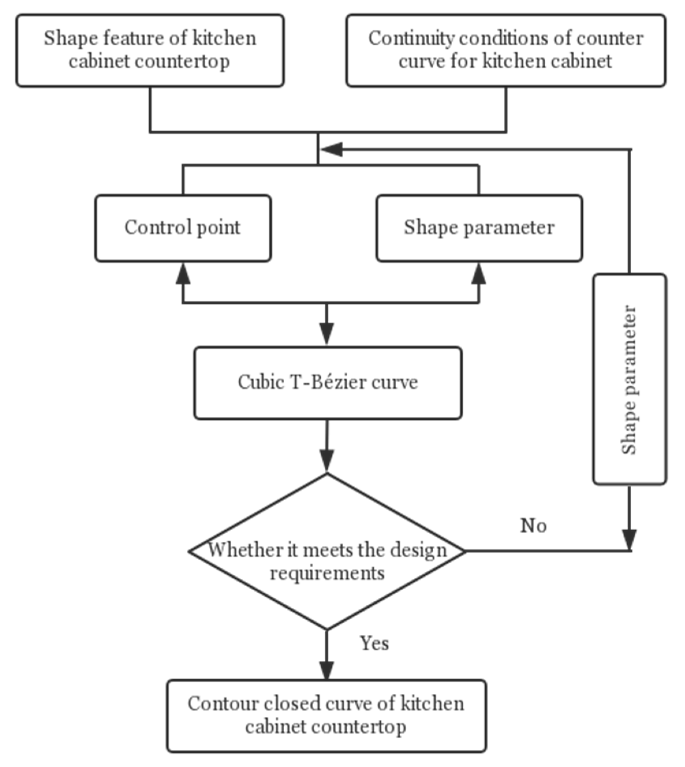
3.1. Construction of Contour Closed Curve of Kitchen Cabinet Countertop

According to the actual needs of life and production, the contour curve of the kitchen cabinet countertop can be regarded as a closed curve that meets certain continuity and smoothness requirements. Since the cubic T-Bézier curve has good shape adjustability and approximation, and can accurately represent a circular arc, it is convenient to design and modify free curves in complex modeling system by using the technique of smooth continuity between two adjacent cubic T-Bézier curves. Therefore, the modeling problem of the contour closed curve of kitchen cabinet countertop can be attributed to the construction problem of the cubic T-Bézier closed curve satisfying certain continuity requirements, and the ideal modeling of a kitchen cabinet counter surface can be obtained by adjusting the shape of the T-Bézier curve. Here, the key to contour curves of kitchen cabinet modeling is the determination of the control points of the T-Bézier curve and the selection of the shape parameters. The specific closed curve modeling process is shown in Figure 4.

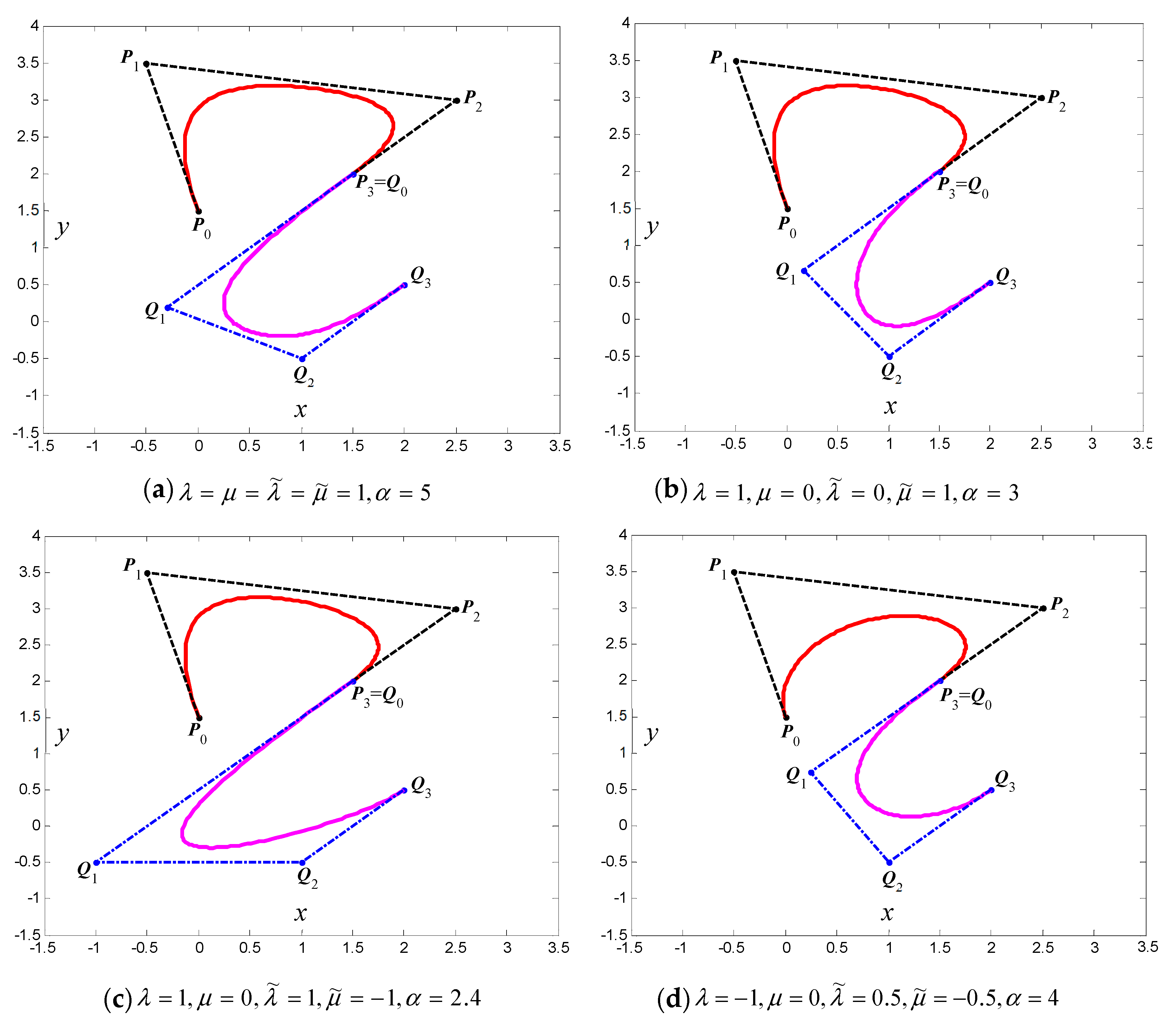
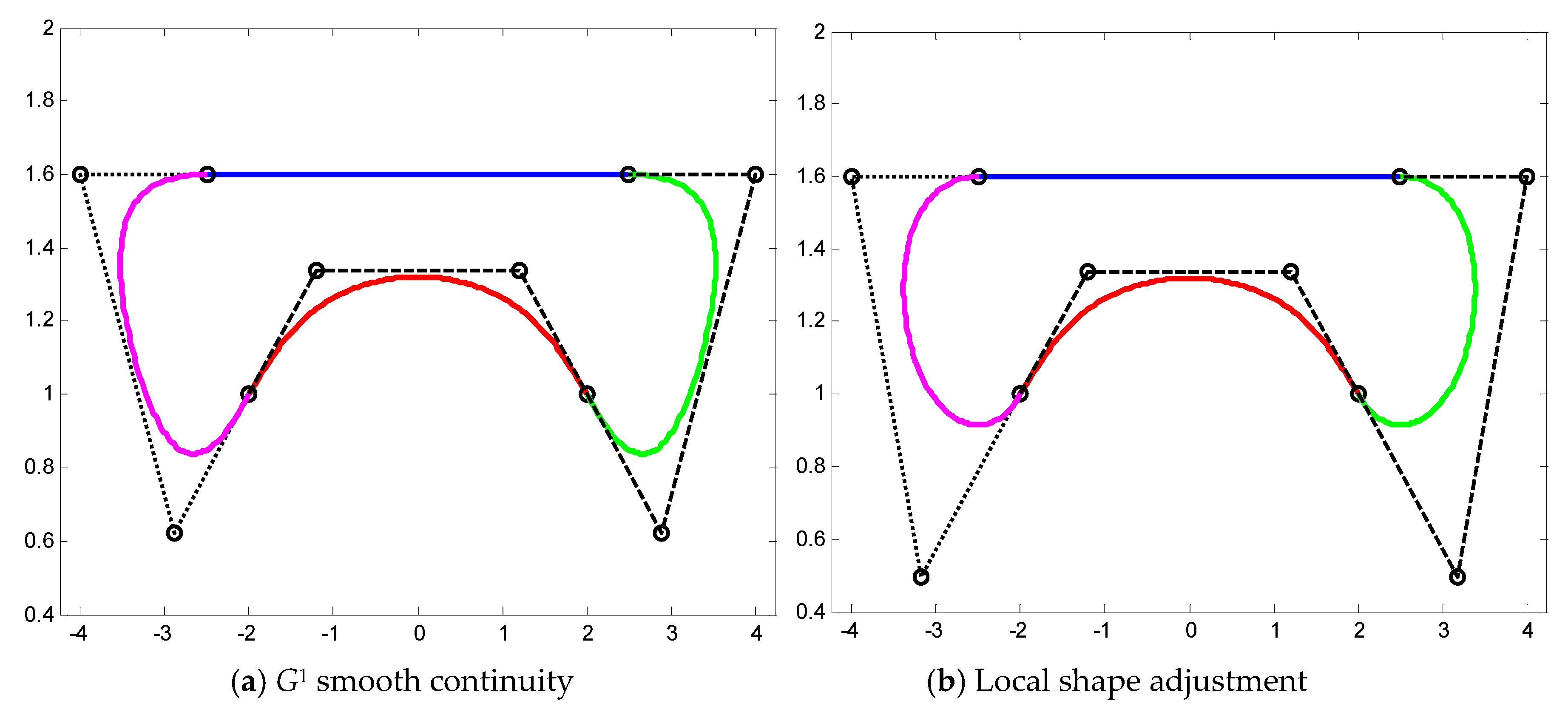
3.1.1. The Contour Closed Curve of Kitchen Cabinet Countertop of G1 Continuity

Based on the cubic T-Bézier model and the smooth continuity conditions discussed above, the steps of constructing the contour closed curve of the kitchen cabinet of G1 continuity are given here. Since the contour closed curve of G1 continuous kitchen cabinet counter surface can be regarded as a composed curve of multiple opened curve that satisfying G1 continuity, it is only necessary to discuss the steps of two adjacent cubic T-Bézier curve r 1 ( t ; λ , μ ) and r 2 ( t ; λ ˜ , μ ˜ ) to achieve G1 smooth continuity. The specific steps are as follows:
Step 1. For two cubic T-Bézier curves r 1 ( t ; λ , μ ) and r 2 ( t ; λ ˜ , μ ˜ ) whose control points are P i ( i = 0 , 1 , 2 , 3 ) and Q i ( i = 0 , 1 , 2 , 3 ) respectively, we first give the initial curve r 1 ( t ; λ , μ ) with the shape parameters λ , μ and the control points P i ( i = 0 , 1 , 2 , 3 ) .
Step 2. According to the condition of smooth continuity between parametric curves, let P 3 = Q 0 , so that r 1 ( t ; λ , μ ) and r 2 ( t ; λ ˜ , μ ˜ ) has a common endpoint, which makes the curves achieve G0 continuity.
Step 3. Given the shape parameter λ ˜ , μ ˜ and scale factor α > 0 of another curve r 2 ( t ; λ ˜ , μ ˜ ) , according to the Equation (5), we can calculate the second control point Q 1 of r 2 ( t ; λ ˜ , μ ˜ ) .
Step 4. The remaining control points Q 2 , Q 3 of the curve r 2 ( t ; λ ˜ , μ ˜ ) are given arbitrarily, and the G1 smooth continuity between two curves r 1 ( t ; λ , μ ) and r 2 ( t ; λ ˜ , μ ˜ ) can be realized at this time.
Step 5. The closed curve (that is, the composed cubic T-Bézier closed curve) in which satisfying G1 continuity is generated.
Step 6. By repeating the steps above, it is possible to achieve G1 smooth continuity between multiple T-Bézier curves, so that composed cubic T-Bézier closed curve in which satisfying G1 smooth continuity is constructed.
In fact, the above steps are only a theoretical method to construct the closed curve of the contour curve for kitchen cabinet, since it is difficult to achieve the desired results at one time. In order to obtain the ideal shape of the kitchen cabinet counter, it is necessary to constantly adjust the shape of the curve locally or wholly, so the good shape adjustability of the cubic T-Bézier curve is particularly important. For the cubic T-Bézier closed curve constructed by the above method, its shape can be adjusted from the following two aspects to obtain the ideal shape of the curve.
(1) First of all, the T-Bézier curve is controlled as a whole by the control points. Since the control point of the curve determines its approximate shape, the contour curve of the kitchen cabinet can be obtained by modifying the control points coordinates of the curve. If the closed curve is required to be G1 continuous, the value of shape parameter can be kept unchanged first, and a control point of T-Bézier curve can be changed arbitrarily, then the adjacent control point also needs to be changed accordingly, so that the G1 continuity requirements can be still met. The adjustment in this respect is relatively tedious. Therefore, the general position of the control point has been determined when the designer sketches the contour curve of the kitchen cabinet counter surface.
(2) Secondly, the T-Bézier curve is adjusted finely by shape parameters. In the shape design of the contour curve of the kitchen cabinet counter surface, the detail adjustment of the curve is a more important step. In the method of constructing the contour modeling of the kitchen cabinet counter surface, it is no need to modify the control vertices, we can adjust the shape of the contour curve well only by modifying the value of the shape parameter of each T-Bézier curve to achieve the purpose of interactive design. It can be seen from the cubic T-Bézier curves with different shape parameters given above that the value of shape parameters is larger, the corresponding curve segment is closer to its control polygon and vice versa. In this aspect of shape adjustment, you can adjust the shape parameter value of each curve segment separately or modify the shape parameter value of the multi curve segment at the same time. The main purpose of introducing shape control parameters λ , μ is to achieve the adjustment of the kitchen cabinet contour curve by simple numerical modification without moving the control points of each curve one by one. It can not only highlight the advantages of parameters contained in the cubic T-Bézier curve but also improve the designer’s work efficiency. By combining the control effect of the control points and shape parameters on the cubic T-Bézier curve, we can construct more abundant and diverse contour modeling of the kitchen cabinet countertop.
Figure 5 shows a modeling example of the contour closed curve with G1 continuous for kitchen cabinet countertop. In Figure 5a, the shape parameters of red curves are λ = μ = 1 , the shape parameters of green and magenta curves are λ ˜ = μ ˜ = 1 and the scale factor is α = 8 ; In Figure 5b, the red curve remains unchanged, and its shape parameters value are also λ = μ = 1 , the shape parameters of green and magenta curves are changed to λ ˜ = 1 , μ ˜ = 0 as well as scale factor is α = 2 , the shape of the composed curve changes at this time. In Figure 5c, the shape parameters of the red curve are λ = μ = 1.3 , the shape parameters of the green and magenta curves are λ ˜ = μ ˜ = 0 . In Figure 5d, the shape parameters of red curves are λ = μ = 0.2 , the shape parameters of green and magenta curves are λ ˜ = μ ˜ = 1 . It can be seen from the figure that when the shape parameters take different values, the contours closed curve of the kitchen cabinet counter surface with different shapes can be obtained, and the transition of the green and magenta splicing curve at two common joints is natural and smooth.

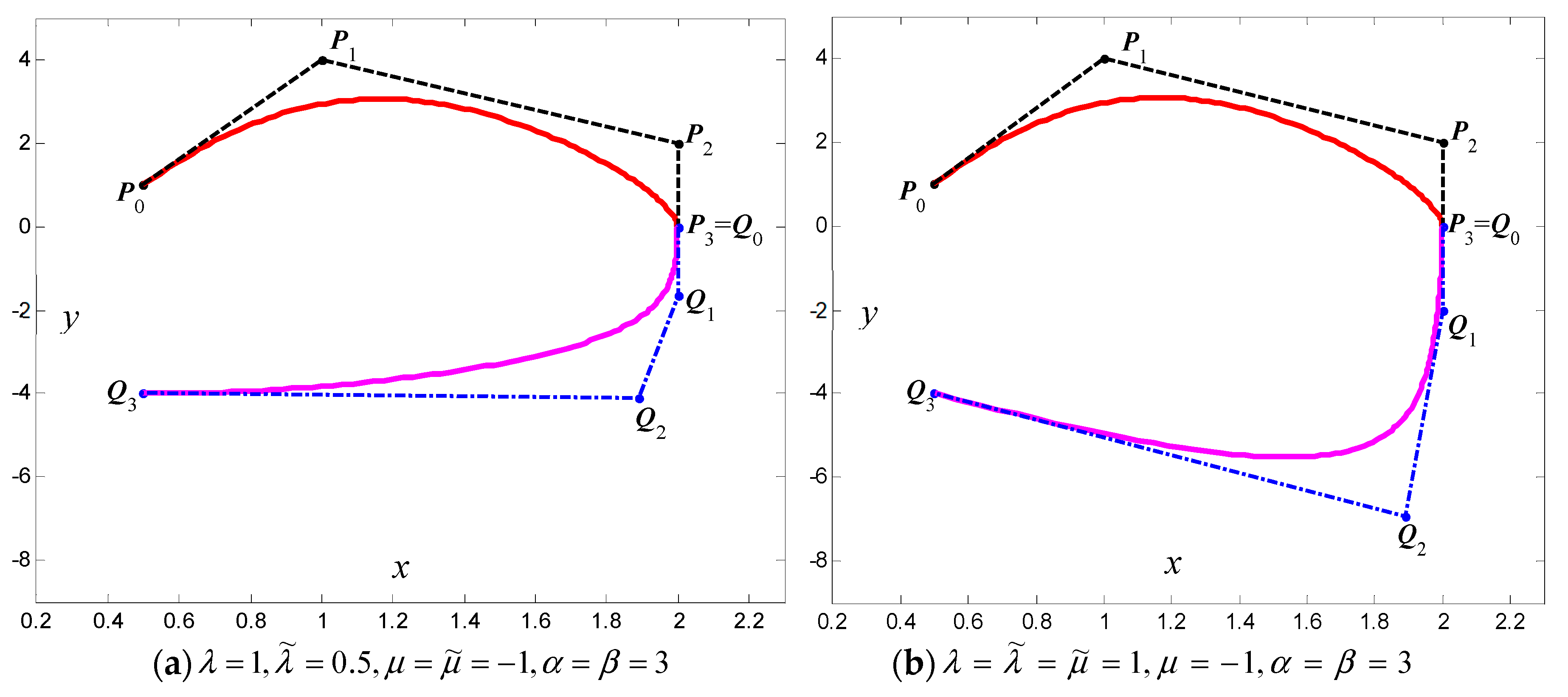
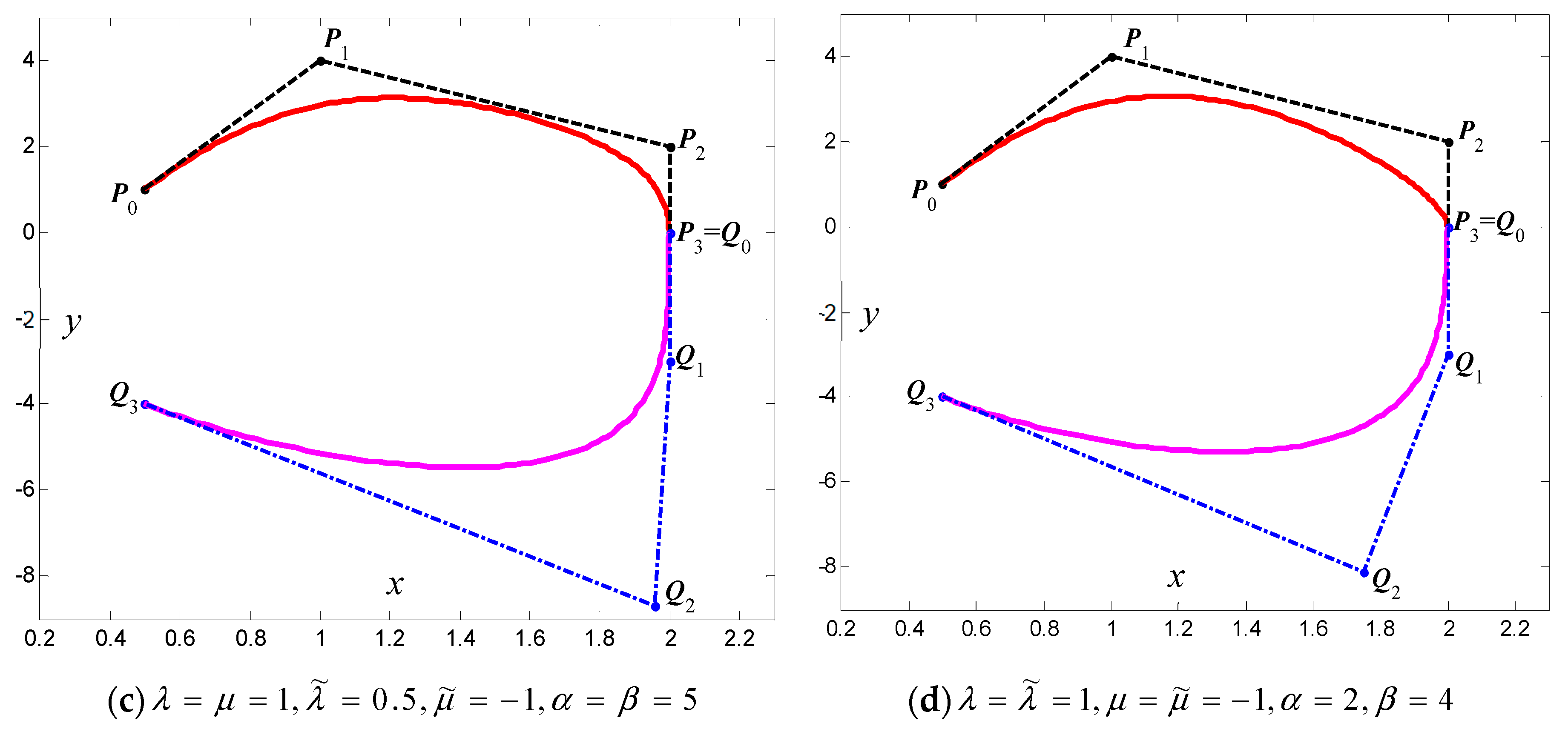
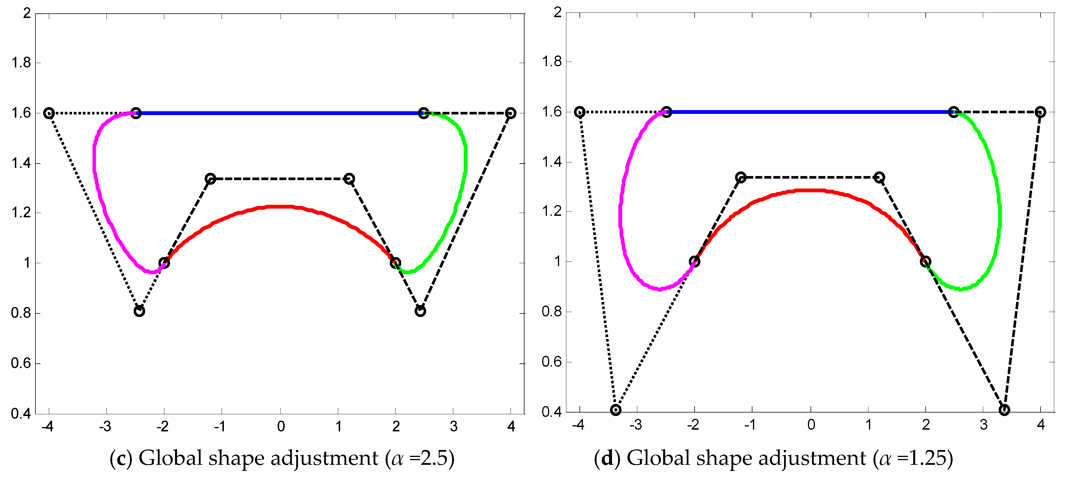
3.1.2. The Contour Closed Curve of Kitchen Cabinet Countertop of G2 Continuity

Similar to the G1 smooth continuity, as long as the G2 smooth continuity steps of two adjacent T-Bézier curves r 1 ( t ; λ , μ ) and r 2 ( t ; λ ˜ , μ ˜ ) are given, the contour modeling of the kitchen cabinet counter surface can be constructed by T-Bézier curves. The steps of T-Bézier curve r 1 ( t ; λ , μ ) and r 2 ( t ; λ ˜ , μ ˜ ) to achieve G2 smooth continuity are as follows:
Step 1. For two cubic T-Bézier curves r 1 ( t ; λ , μ ) and r 2 ( t ; λ ˜ , μ ˜ ) whose control points are P i ( i = 0 , 1 , 2 , 3 ) and Q i ( i = 0 , 1 , 2 , 3 ) respectively, we first give the initial curve r 1 ( t ; λ , μ ) with the shape parameters λ , μ and the control points P i ( i = 0 , 1 , 2 , 3 ) .
Step 2. According to the condition of smooth continuity between parametric curves, let P 3 = Q 0 , so that r 1 ( t ; λ , μ ) and r 2 ( t ; λ ˜ , μ ˜ ) have a common endpoint, which makes the curves achieve G 0 continuity.
Step 3. Given the shape parameters λ ˜ , μ ˜ and scale factor α > 0 of another curve r 2 ( t ; λ ˜ , μ ˜ ) , according to Equation (5), we can calculate the second control point Q 1 of r 2 ( t ; λ ˜ , μ ˜ ) .
Step 4. On the basis of the above steps, if the constant β is given, according to Equation (5), the third control point Q 2 of the curve r 2 ( t ; λ ˜ , μ ˜ ) can be obtained.
Step 5. Finally, the remaining control points Q 3 of the curve r 2 ( t ; λ ˜ , μ ˜ ) are given arbitrarily, and the G2 smooth continuity between two curves r 1 ( t ; λ , μ ) and r 2 ( t ; λ ˜ , μ ˜ ) can be realized at this time.
Step 6. In the same way, by repeating the steps above, it is possible to construct composed curves which satisfy the G2 smooth continuity.
Based on the above construction steps of the G2 continuous composed closed curve, Figure 6 shows an example of contour modeling with G2 continuity for kitchen cabinet countertop. In Figure 6a, the shape parameters of the red and green curves are λ = 1 , μ = 1 , the shape parameters of the magenta and blue curves are λ ˜ = 1 , μ ˜ = 1 and the scale factors are α = 2 , β = 8 . In Figure 6b, the shape parameters of each cubic T-Bézier curve are equal to those in Figure 6a, but as the scale factors are α = 2 , β = 6 , the shape of the composed curve changes at this time. In Figure 6c,d, the shape parameters of the red and green curves are λ = 1 , μ = 1 , the shape parameters of the magenta and blue curves in Figure 6c,d are λ ˜ = 1 , μ ˜ = 0 , λ = 1 , μ = 1 respectively and scale factors are α = 2 , β = 10 , α = 3 , β = 5 . The polylines and dots in Figure 6 have the same meaning as in Figure 5. It can be seen from the figure that we can modify the local or global shape of the composed closed curve by changing the value of the shape parameter without changing the continuity conditions of the curve, which is undoubtedly the most important feature in practical application.

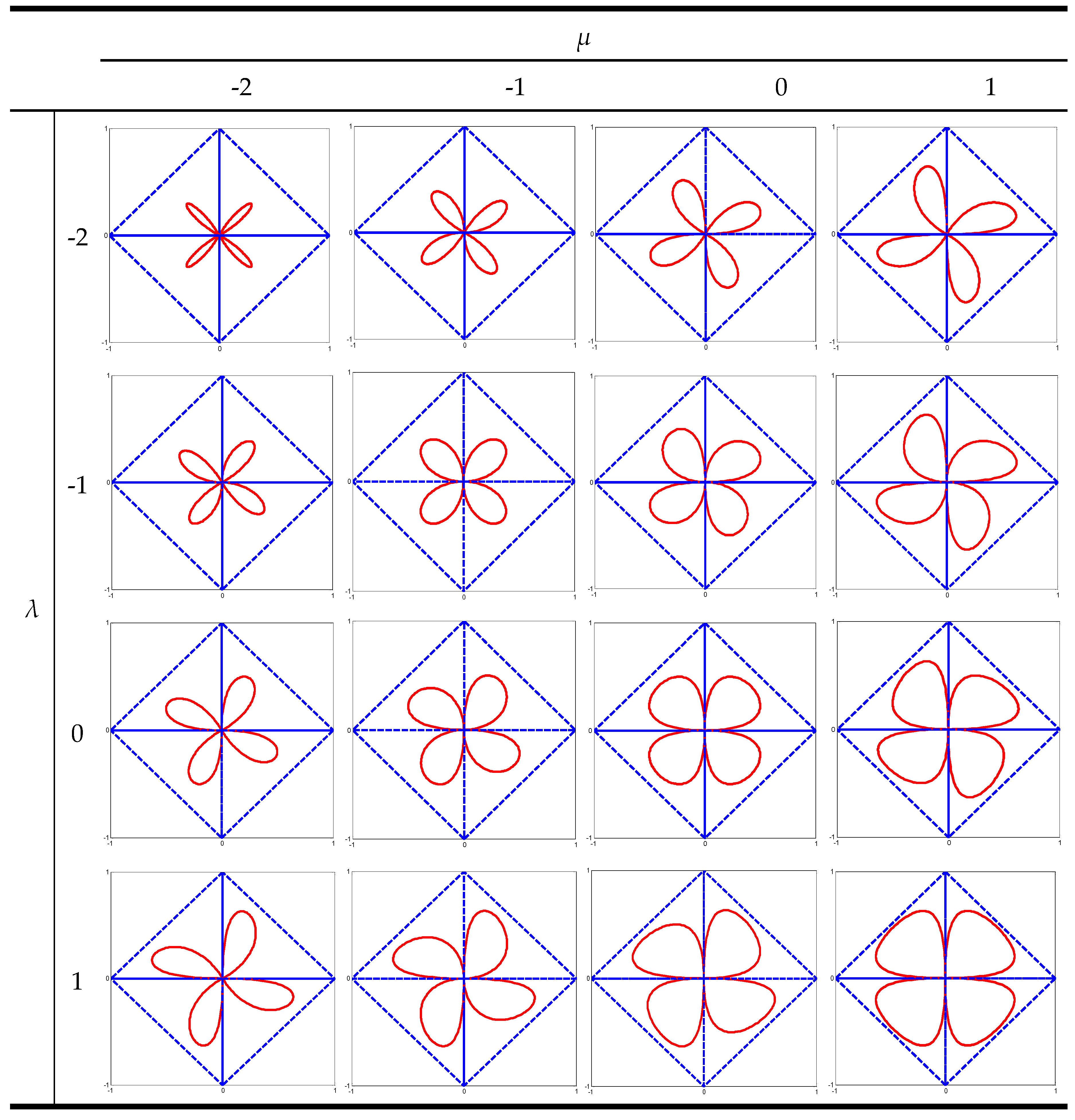
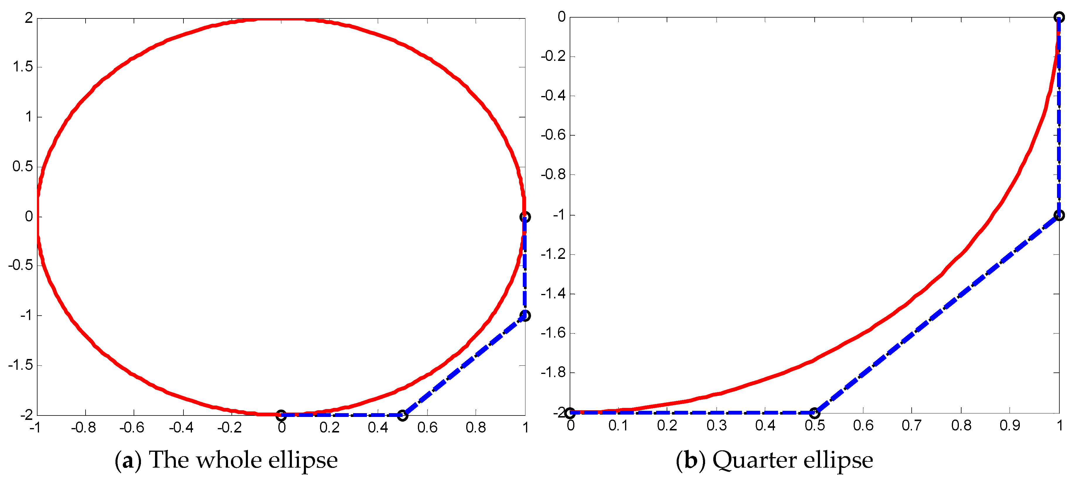
3.2. The Representation of Ellipses with Cubic T-Bézier Curves

Theorem 4.
Let P 0 , P 1 , P 2 , P 3 be the four control points on an ellipse with semi-axes a and b , and take its coordinates as
P 0 = ( a 0 ) , P 1 = ( a b 2 ) , P 2 = ( a 2 b ) , P 3 = ( 0 b ) .
Here, λ = μ = 0 , t [ t 1 , t 2 ] , then the T-Bézier curve with P 0 , P 1 , P 2 , P 3 as the control points is the elliptical arc
r x ( t ) = a cos π 2 t , r y ( t ) = b sin π 2 t ,
where 0 t 1 , t 2 1 .
Proof. 
Substituting P 0 = ( a 0 ) , P 1 = ( a b 2 ) , P 2 = ( a 2 b ) , P 3 = ( 0 b ) into Equation (2), then the coordinates of T-Bézier curve can be obtained as follows
{ x ( t ) = a cos π 2 t , y ( t ) = b sin π 2 t .
This gives the intrinsic equation
( x a ) 2 + ( y b ) 2 = 1 .
This is an elliptic equation, so Theorem 4 is proved. □
Remark 1.
Since Equation (16) only represents the first quadrant of an ellipse, which is often insufficient in practical applications. To represent an entire ellipse or part of an ellipse, the following can be performed:
(1) If you want to represent the whole ellipse, you only need to extend the value of the variable in Equation (16) to [ 0 , 4 ] (see Figure 7a).
(2) If you want to represent a partial elliptic arc with a central angle of θ [ θ 1 , θ 2 ] you only need to take t [ 2 θ 1 π , 2 θ 2 π ] correspondingly (see Figure 7b).
Figure 7 shows the representation of ellipses with T-Bézier curves, where t [ 0 , 4 ] (left) and t [ 0 , 1 ] (right). Figure 8a,b gives the contour closed curve modeling of kitchen cabinet counter surface with partial elliptic arcs, where the red curve represents the partial elliptic arc corresponding to t [ 0.4 , 1.9 ] and the magenta curves represent the cubic T-Bézier curves corresponding to the shape parameters λ = 1 , μ = 1 and λ = 1 , μ = 0 , respectively. It can be seen from the figure that when the ideal kitchen cabinet contour model contains an elliptic arc, it can be expressed accurately by using the cubic T-Bézier curve, which is also one of the advantages of using cubic T-Bézier curve to construct the contour curve of kitchen cabinet counter model.

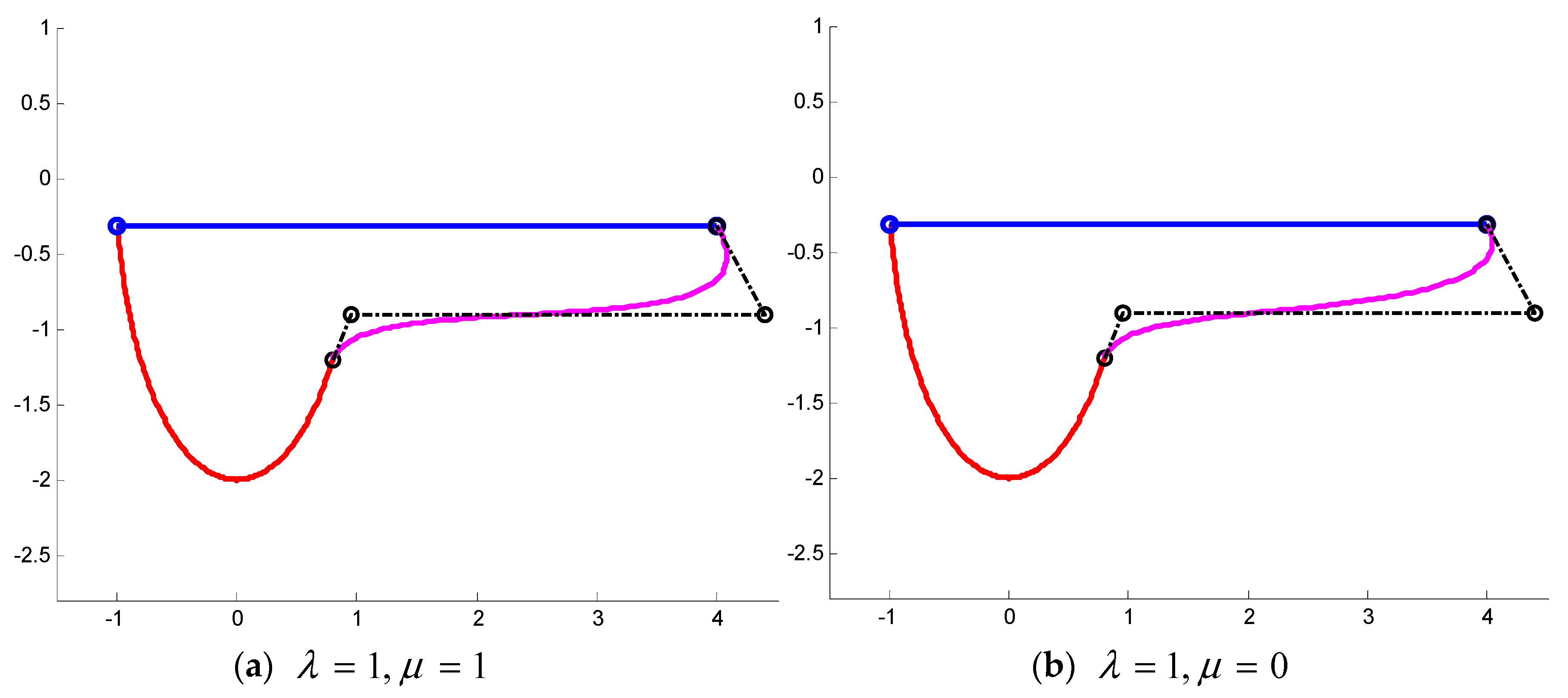
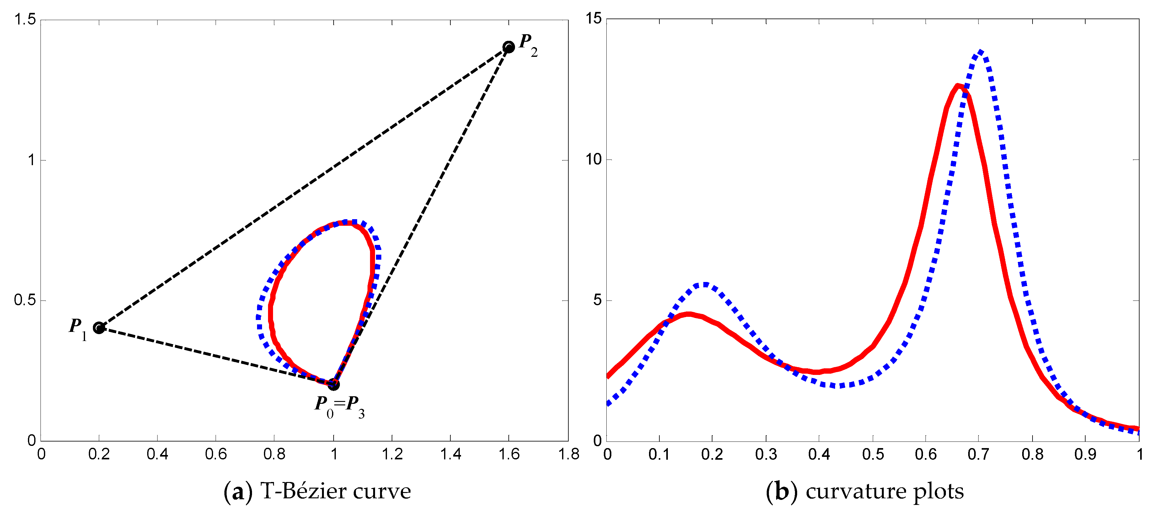
3.3. Shape Optimization of Cubic T-Bézier Curves

In this section, we mainly use the idea of energy minimization to construct the optimal cubic T-Bézier curve, so as to optimize the shape of the cubic T-Bézier curve. The specific methods are as follows: by minimizing the energy of approximate curvature variation, the optimal values of the two shape parameters of the cubic T-Bézier curve are determined, and then an optimized cubic T-Bézier curve is obtained.
According to the literature [32], the curvature variation energy of cubic T-Bézier curve r 1 ( t ; λ , μ ) can be defined as
E = 0 1 ( κ ( t ) ) 2 d t ,
where κ ( t ) = | | r ( t ) × r ( t ) | | | | r ( t ) | | 3 , and κ ( t ) is the first derivative of κ ( t ) , r ( t ) as well as r ( t ) represents the first and the second derivative of r ( t ) , respectively.
Since the curvature variation energy in Equation (19) is highly nonlinear, we can use some approximate forms to simplify the calculation. In [33,34], the curvature variation energy is expressed in the following form
E ^ = 0 1 r ( t ) 2 d t .
Theorem 5.
The curvature variation energy of a cubic T-Bézier curve defined by Equation (2) is minimum if and only if
λ = a 2 a 4 a 1 a 3 a 0 a 1 a 2 2 , μ = a 2 a 3 a 0 a 4 a 0 a 1 a 2 2 .
where a i , i = 0 , 1 , 4 are calculated as follows:
{ a 0 = π 5 15360 ( 13515 π 29696 ) Δ p 0 2 , a 1 = π 5 15360 ( 13515 π 29696 ) Δ p 2 2 , a 2 = π 5 1920 ( 960 π 3367 ) Δ p 0 Δ p 2 , a 3 = π 5 3840 ( ( 3136 1065 π ) p 0 + ( 4992 + 2025 π ) p 1 + ( 3972 1920 π ) p 2 + ( 2116 + 960 π ) p 3 ) Δ p 0 , a 4 = π 5 3840 ( ( 2116 960 π ) p 0 + ( 3972 + 1920 π ) p 1 + ( 4992 2025 π ) p 2 + ( 3136 + 1065 π ) p 3 ) Δ p 2 .
Proof. 
First, we consider the expression of curvature variation energy of the cubic T-Bézier curve. For the convenience of calculation, we can rewrite Equation (2) as follows
{ b 0 ( t ) = ( 1 sin π 2 t ) 2 λ sin π 2 t ( 1 sin π 2 t ) 2 , b 1 ( t ) = 2 sin π 2 t ( 1 sin π 2 t ) + λ sin π 2 t ( 1 sin π 2 t ) 2 , b 2 ( t ) = 2 cos π 2 t ( 1 cos π 2 t ) + μ cos π 2 t ( 1 cos π 2 t ) 2 , b 3 ( t ) = ( 1 cos π 2 t ) 2 μ cos π 2 t ( 1 cos π 2 t ) 2 .
It can be seen that Equation (23) is more concise and intuitive than Equation (1). By Equation (23), Equation (2) can be expressed as
r ( t ) = λ a ( t ) Δ P 0 + μ b ( t ) Δ P 2 + s ( t ) ,
where Δ P 0 = P 1 P 0 , Δ P 2 = P 3 P 2 , which are vector differences between the corresponding control points and
{ a ( t ) = sin π 2 t ( 1 sin π 2 t ) 2 , b ( t ) = cos π 2 t ( 1 cos π 2 t ) 2 , s ( t ) = ( 1 sin π 2 t ) 2 P 0 + 2 sin π 2 t ( 1 sin π 2 t ) P 1 + 2 cos π 2 t ( 1 cos π 2 t ) P 2 + ( 1 cos π 2 t ) 2 P 3 .
By Equation (24), the integral function in the expression of curvature variation energy of the cubic T-Bézier curve can be obtained as follows
r ( t ) 2 = λ a ( t ) Δ P 0 + μ b ( t ) Δ P 2 + s ( t ) 2 = λ 2 ( a ( t ) Δ P 0 ) 2 + μ 2 ( b ( t ) Δ P 2 ) 2 + 2 λ μ ( a ( t ) Δ P 0 ) ( b ( t ) Δ P 2 ) + 2 λ a ( t ) Δ P 0 s ( t ) + 2 μ b ( t ) Δ P 2 s ( t ) + s ( t ) 2 .
For given control points of pi (i = 0, 1, 2, 3), we have
a 0 = 0 1 ( a ( t ) Δ P 0 ) 2 d t = π 5 15360 ( 13515 π 29696 ) Δ P 0 2 ,
a 1 = 0 1 ( b ( t ) Δ P 2 ) 2 d t = π 5 15360 ( 13515 π 29696 ) Δ P 2 2 ,
a 2 = 0 1 ( a ( t ) Δ P 0 ) ( b ( t ) Δ P 2 ) d t = π 5 1920 ( 960 π 3367 ) Δ P 0 Δ P 2 ,
a 3 = 0 1 a ( t ) Δ P 0 s ( t ) d t = π 5 3840 ( ( 3136 1065 π ) P 0 + ( 4992 + 2025 π ) P 1 + ( 3972 1920 π ) P 2 + ( 2116 + 960 π ) P 3 ) Δ P 0 ,
a 4 = 0 1 b ( t ) Δ P 2 s ( t ) d t = π 5 3840 ( ( 2116 960 π ) P 0 + ( 3972 + 1920 π ) P 1 + ( 4992 2025 π ) P 2 + ( 3136 + 1065 π ) P 3 ) Δ P 2 ,
a 5 = 0 1 S ( t ) 2 d t .
Substituting Equation (25) into Equation (20), and combining with Equations (26)–(31), the curvature variation energy of cubic T-Bézier curve r ( t ; λ , μ ) can be simplified as follows:
E ^ = 0 1 r ( t ) 2 d t = λ a ( t ) Δ P 0 + μ b ( t ) Δ P 2 + s ( t ) 2 = λ 2 ( a ( t ) Δ P 0 ) 2 + μ 2 ( b ( t ) Δ P 2 ) 2 + 2 λ μ ( a ( t ) Δ P 0 ) ( b ( t ) Δ P 2 ) + 2 λ a ( t ) Δ P 0 s ( t ) + 2 μ b ( t ) Δ P 2 s ( t ) + s ( t ) 2 = λ 2 a 0 + μ 2 a 1 + 2 λ μ a 2 + 2 λ a 3 + 2 μ a 4 + a 5 .
Therefore, we can get the following functions by Equation (32),
f ( λ , μ ) = 0 1 r ( t ) 2 d t a 5 = λ 2 a 0 + μ 2 a 1 + 2 λ μ a 2 + 2 λ a 3 + 2 μ a 4 .
Since we want to minimize the energy function of approximate curvature variation to obtain the optimal values of two free parameters, the following optimization models can be obtained
{ min   f ( λ , μ ) = λ 2 a 0 + μ 2 a 1 + 2 λ μ a 2 + 2 λ a 3 + 2 μ a 4 , s . t . ( λ , μ ) [ 2 , 1 ] × [ 2 , 1 ] .
The Hessian matrix of Equation (33) is
H = 2 ( a 0 a 2 a 2 a 1 ) ,
when Pi (i = 0,1,2,3) takes different values, it can be easily checked that a0 > 0 and a0a1a22 > 0. That is to say, the determinant value of the matrix H is det(H) = 0, which means that the matrix H is symmetrical positive definite.
Since Equation (33) is a quadratic function and the remainder of the second-order Taylor expansion of function f ( λ , μ ) is equal to zero, it is obtained from the relationship between the semi-positive definite matrix and the extreme point that the quadratic function f ( λ , μ ) has a minimum value at the extreme point. Because of the differentiability of the function f ( λ , μ ) , we know that the minimum value of the function f ( λ , μ ) is the minimum value of the optimization model in Equation (34), i.e., the optimal solution.
The gradients of Equation (33) can be calculated by
f λ = 2 λ a 0 + 2 μ a 2 + 2 a 3 , f μ = 2 λ a 2 + 2 μ a 1 + 2 a 4 .
From the relationship between semi-positive definite matrix and extremum, we can see that the following unique solution of Equation (34) can be solved from f = 0 with the gradient expression in Equation (36),
λ ^ = a 2 a 4 a 1 a 3 a 0 a 1 a 2 2 , μ ^ = a 2 a 3 a 0 a 4 a 0 a 1 a 2 2 .
This completes the proof. □
For the given control points, we can directly derive the values of each real constant a i ( i = 0 , 1 , 2 , 3 ) and substitute it into Equation (29) to obtain the optimal values of two shape parameters, thus a cubic T-Bézier curve can be drawn, which the curvature variation energy of the curve is minimum.
Then, some numerical examples of the cubic T-Bézier curve with minimum curvature variation energy are given. First of all, we take the coordinates of the control points of the curve. Secondly, we can get the optimal values of two shape parameters according to the coordinates. Then, we can draw the optimized curve by substituting the optimal values of the shape parameters into the definition expression of the cubic T-Bézier curve, and the traditional cubic Bézier curve and the corresponding curvature graph can be drawn as well. Given a cubic T-Bézier closed curve, which coordinates of its control points are P 0 = P 3 = ( 1 , 0.2 ) , P 1 = ( 0.2 , 0.4 ) , P 2 = ( 1.6 , 1.4 ) , then according to Equation (29), the optimal approximate solution of two shape parameters can be obtained as λ = 0.6988 , μ = 0.5359 . Figure 9 shows the cubic T-Bézier curve and the traditional cubic Bézier curve which obtained by minimizing the energy of approximate curvature variation, and their corresponding curvature graphs.
Similarly, for the cubic T-Bézier opened curve with different shape parameters given in Figure 2, the optimal values of the two shape parameters of the cubic T-Bézier curve calculated by Equation (29) are λ = 0.0215 , μ = 0.4889 . Figure 10 shows two cubic T-Bézier opened curves and corresponding traditional cubic Bézier curves obtained by minimizing the energy of approximate curvature variation, as well as their corresponding curvature plots, which are similar to the heart shape.
Similarly, for the contour closed curve of the kitchen cabinet of G 1 continuity given in Figure 5, the optimal values of the two shape parameters of the red, magenta and green cubic T-Bézier curves are calculated by (29), that is
λ = μ = 0.8081 ; λ ˜ = 0.3507 , μ ˜ = 0.1028 ; λ ˜ = 0.3507 , μ ˜ = 0.1028 .
For the contour closed curve of the kitchen cabinet of G 2 continuity given in Figure 6, the optimal values of the two shape parameters of the red and green cubic T-Bézier curves are calculated by Equation (29), i.e., λ = 0.0938 , μ = 0.0458 , the optimal values of the two shape parameters of magenta and green cubic T-Bézier curves are calculated are λ = 0.8509 , μ = 0.1395 .
Based on the cubic T-Bézier curve, Figure 11 gives an example of optimal modeling of G1 and G2 continuity closed curves of kitchen cabinet countertop by minimizing the energy of approximate curvature variation, meanwhile corresponding traditional cubic Bézier curves are given as well.

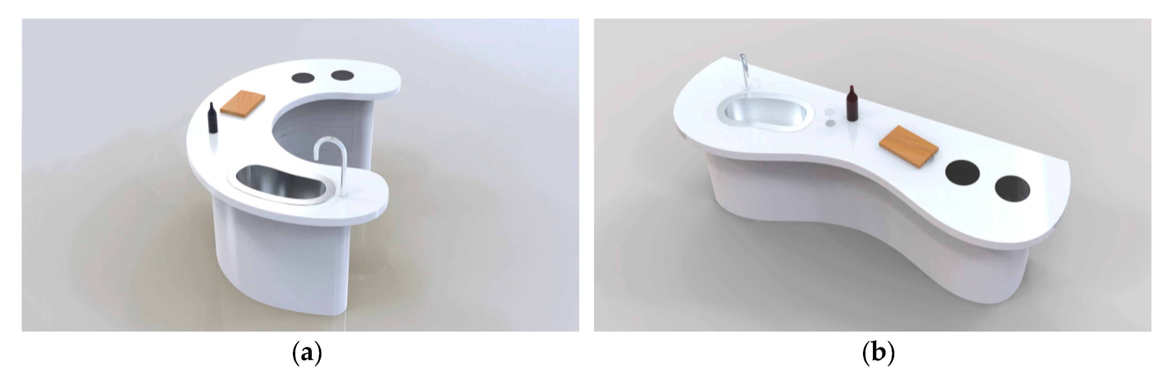
4. Examples of Kitchen Cabinet Design

As an important part of people’s kitchen products, the kitchen cabinet has been constantly updated in recent years. With the change of users’ lifestyles, their demands for kitchen products in terms of function, structure and visual communication are also getting higher. At present, the homogenization of kitchen cabinet products in the market is serious, as most of them are fixed-cuboid modules according to the kitchen space. In the current situation of increasing personal needs, kitchen cabinets should not be limited to straight lines with sharp edges, as a curved kitchen countertop looks freer, smooth and reasonable. The main modeling element of the curved kitchen cabinet is the outline which describes the appearance of the countertop, that is, the product’s modeling feature line, so how to determine it is the most important part of the design process. As an extension of the Bézier model, the T-Bézier model can provide an efficient tool for the development of CAD software, which plays a key role in fields such as product design, manufacturing industry, etc. By using the presented methods in this paper, we can expediently design various kinds of kitchen cabinet countertop outlines. In this section, we will give some convictive examples to illustrate the effectiveness of our proposed methods.
Figure 12 gives some examples to design the contour curves of the kitchen cabinet by using T-Bézier curves. In Figure 12, each contour curve is composed of multiple T-Bézier curves with G1 or G2 smooth continuity. As can be seen from Figure 12, designers can use control points to draw the initial shapes of contour curves of kitchen cabinet, and then the ultimate shapes of the contour curves can be obtained quickly by adjusting multiple local shape parameters. In the kitchen cabinet modeling design, kitchen cabinet contour is undoubtedly the most important part of the kitchen cabinet body, and the contour curves is a vital visual feature in the kitchen cabinet modeling. Figure 13 shows an application of parametric modeling for kitchen cabinet design by using the T-Bézier model. As shown in Figure 13, various styles of kitchen cabinet modeling schemes with optimal shape can be obtained by using the methods proposed in this paper. Figure 14 shows the scene effect of a curved kitchen cabinet in a specific residential space, it can be seen that the kitchen cabinet product matches the surrounding space environment very well.

5. Conclusions

The local controlled T-Bézier model inherits beneficial properties of the classical Bézier one, but its entire performance is superior to that of the Bézier model. In this paper, we presented an efficient parametric method to design the contour curves of kitchen cabinet by using cubic T-Bézier curves with local shape parameters, and studied shape optimization and representation of ellipses for the contour curves of the kitchen cabinet. We feel our work is significant since our proposals help to expediently and efficiently accomplish the parametric design of kitchen cabinet products. Some representative and convictive examples show the effectiveness of the proposed parametric design method. This method can quickly design kitchen cabinet products with novel styles, which makes up for the current situation that the design of kitchen cabinet products in the market is single and cannot meet the individual and diversified needs of users, and plays an important role in people’s production and life. Our presented T-Bézier model-based parametric design method is better than the traditional design method for kitchen cabinet products. Compare to the traditional design method, our proposed method overcomes the disadvantages of difficult to modify and optimize product shapes designed by traditional methods. The advantages of the proposed method can be summarized as follows:
(1)
Our proposed G1 and G2 continuity conditions for cubic T-Bézier curves extend the conclusions of continuity condition given in [25]; the closed composite cubic T-Bézier curves have a more powerful shape adjustability than the classical composite Bézier curves.
(2)
For a contour curve of kitchen cabinets, designers can adjust the global and local shape of the curve by changing the multiple shape parameters.
(3)
Our proposed method not only quickly obtained various styles of kitchen cabinet modeling schemes but also easily realized the shape optimization design by finding optimal shape parameters.
(4)
The proposed method in this paper is easy to apply or extend to the parametric design of other products.
It is worth noting we are the first to study the curve model-based parametric design for kitchen cabinet products. The proposed method is not limited to the design of kitchen cabinets, it can also be applied to various products with curved shapes. The T-Bézier model is not only used for kitchen parametric modeling but also for CAD modeling in the field of mechanical engineering. Another interesting direction for future research can be from the perspective of internal kitchen design and the sustainable development of energy balance [35], moreover, the parametric design of more complex kitchen products can be achieved by using T-Bézier surfaces with local shape parameters.

Author Contributions

All authors contributed equally to the writing of this paper. All authors read and approved the final manuscript.

Funding

This work is supported by the Shaanxi Social Science Fund Project (Grant No. 2019K033).

Acknowledgments

We thank the anonymous reviewers for their important and valuable suggestions, which led to the improvements in the presentation of this paper.

Conflicts of Interest

The authors declare that there is no conflict of interest regarding the publication of this paper.

References

  1. Millman, D. Brand Thinking and Other Noble Pursuits: Insights and Provocations from World-Renowned Brand Consultants, Thought Leaders Designers, and Strategists; All Worth Press: New York, NY, USA, 2011. [Google Scholar]
  2. Berghman, M.; Hekkert, P. Towards a unified model of aesthetic pleasure in design. New Ideas Psychol. 2017, 47, 136–144. [Google Scholar] [CrossRef]
  3. Moulson, T.; Sproles, G. Styling strategy. Bus. Horiz. 2000, 43, 45–52. [Google Scholar] [CrossRef]
  4. Farin, G. Curves and Surfaces for CAGD: A Practical Guide, 5th ed.; Academic Press: San Diego, CA, USA, 2002. [Google Scholar]
  5. Tovey, M. Computer-aided vehicle styling. Comput. Aided Des. 1989, 21, 172–179. [Google Scholar] [CrossRef]
  6. Oxman, R. Thinking difference: Theories and models of parametric design thinking. Des. Stud. 2017, 52, 4–39. [Google Scholar] [CrossRef]
  7. Shajay, B. Parametric design thinking: Symmetry a case-study of practice-embedded architectural research. Des. Stud. 2017, 52, 115–143. [Google Scholar]
  8. Hyun, K.H.; Lee, J.H. Balancing homogeneity and heterogeneity in design exploration by synthesizing novel design alternatives based on genetic algorithm and strategic styling decision. Adv. Eng. Inform. 2018, 38, 113–128. [Google Scholar] [CrossRef]
  9. Padmanabhan, R.; Oliveira, M.C.; Baptista, A.J.; Alves, J.L.; Menezes, L.F. Blank design for deep drawn parts using parametric NURBS surfaces. J. Mater. Process. Technol. 2009, 209, 2402–2411. [Google Scholar] [CrossRef] [Green Version]
  10. Wang, C.C.L. Parameterization and parametric design of mannequins. Comput. Aided Des. 2005, 37, 83–98. [Google Scholar] [CrossRef]
  11. Huang, J.; Kwok, T.H.; Zhou, C. Parametric design for human body modeling by wireframe-assisted deep learning. Comput. Aided Des. 2018, 108, 19–29. [Google Scholar] [CrossRef]
  12. Pérez-Arribas, F.; Pérez-Fernández, R. A B-spline design model for propeller blades. Adv. Eng. Softw. 2018, 118, 35–44. [Google Scholar] [CrossRef]
  13. Koini, G.N.; Sarakinos, S.S.; Nikolos, I.K. A software tool for parametric design of turbomachinery blades. Adv. Eng. Softw. 2009, 40, 41–51. [Google Scholar] [CrossRef]
  14. Yu, S.L.; Wang, Z.W.; Li, J. NURBS on the design of the horse-hoof-shaped leg. J. Nanjing For. Univ. 2001, 25, 77–79. [Google Scholar]
  15. Khan, S.; Gunpinar, E.; Dogan, K.M. A novel design framework for generation and parametric modification of yacht hull surfaces. Ocean Eng. 2017, 136, 243–259. [Google Scholar] [CrossRef] [Green Version]
  16. Merrell, P.; Dinesh, M. Example-based curve synthesis. Comput. Graph. 2010, 34, 304–311. [Google Scholar] [CrossRef]
  17. Hu, G.; Wu, J.L.; Qin, X.Q. A novel extension of the Bézier model and its applications to surface modeling. Adv. Eng. Softw. 2018, 125, 27–54. [Google Scholar] [CrossRef]
  18. Hu, G.; Bo, C.; Wu, J.; Wei, G.; Hou, F. Modeling of free-form complex curves using SG-Bézier curves with constraints of geometric continuities. Symmetry 2018, 10, 545. [Google Scholar] [CrossRef] [Green Version]
  19. Liu, F.; Ji, X.; Hu, G.; Gao, J. A novel shape-adjustable surface and its applications in car design. Appl. Sci. 2019, 9, 2339. [Google Scholar] [CrossRef] [Green Version]
  20. Guo, L.; Zhao, J.; Hu, G. Ceramic product form design based on quartic ω-Bézier curves. China Ceram. 2015, 51, 41–44. [Google Scholar]
  21. Zhou, M.; Yang, J.Q.; Zheng, H.C.; Song, W.J. Design and shape adjustment of developable surfaces. Appl. Math. Model. 2013, 37, 3789–3801. [Google Scholar] [CrossRef]
  22. Hu, G.; Cao, H.X.; Qin, X.Q.; Wang, X. Geometric design and continuity conditions of developable λ-Bézier surfaces. Adv. Eng. Softw. 2017, 114, 235–245. [Google Scholar] [CrossRef]
  23. Hu, G.; Wu, J.L.; Qin, X.Q. A new approach in designing of local controlled developable H-Bézier surfaces. Adv. Eng. Softw. 2018, 121, 26–38. [Google Scholar] [CrossRef]
  24. Hu, G.; Wu, J.L. Generalized quartic H-Bézier curves: Construction and application to developable surfaces. Adv. Eng. Softw. 2019, 138, 102723. [Google Scholar] [CrossRef]
  25. Han, X.A.; Ma, Y.C.; Huang, X.L. The cubic trigonometric Bézier curve with two shape parameters. Appl. Math. Lett. 2009, 22, 226–231. [Google Scholar] [CrossRef] [Green Version]
  26. Li, J.C. Planar T-Bézier curve with approximate minimum curvature variation. J. Adv. Mech. Des. Syst. 2018, 12, 1–7. [Google Scholar] [CrossRef] [Green Version]
  27. Huang, J.; Li, Z.; Hu, J.L. Research on connection conditions of two T-Bézier surfaces and its application in textile modeling. Comput. Eng. Des. 2009, 32, 481–486. [Google Scholar]
  28. Liu, F.; Ji, X.M.; Gong, L.Q. A CAD modeling method for car form design based on CE-Bézier. In Proceedings of the 11th International Conferences on Computer Graphics, Visualization, Computer Vision and Image Processing (IADIS: 2017), Lisbon, Portugal, 21 July 2017. [Google Scholar]
  29. Guo, L.; Ji, X.M.; Hu, G.; Chu, J.J. Car headlight shape design based on cubic Q-Bézier curves. China Mech. Eng. 2013, 24, 1961–1969. [Google Scholar]
  30. Gao, J.; Cui, Y.; Ji, X.; Wang, X.; Hu, G.; Liu, F. A Parametric Identification Method of Human Gait Differences and its Application in Rehabilitation. Appl. Sci. 2019, 9, 4581. [Google Scholar] [CrossRef] [Green Version]
  31. Hwang, J.H.; Lee, H. Parametric Model for Window Design Based on Prospect-Refuge Measurement in Residential Environment. Sustainability 2018, 10, 3888. [Google Scholar] [CrossRef] [Green Version]
  32. Farin, G. Geometric Hermite interpolation with circular precision. Comput. Aided Geom. Des. 2008, 40, 476–479. [Google Scholar] [CrossRef] [Green Version]
  33. Lu, L.Z. A note on curvature variation minimizing cubic Hermite interpolants. Appl. Math. Comput. 2015, 259, 596–599. [Google Scholar] [CrossRef]
  34. Lu, L.Z.; Jiang, C.K.; Hu, Q.Q. Planar cubic G1 and quintic G2 Hermite interpolations via curvature variation minimization. Comput. Graph. 2017, 70, 92–98. [Google Scholar] [CrossRef]
  35. Lucchi. Non-invasive method for investigating energy and environmental performances in existing buildings. In PLEA 2011-Architecture and Sustainable Development, Conference Proceedings of the 27th International Conference on Passive and Low Energy Architecture; Altamira Press: Brussels, Belgium, 2011. [Google Scholar]
Figure 1. The cubic T−Bézier curve with different shape parameters (closed curve).
Symmetry 12 00505 g001
Figure 2. smooth continuity of cubic T-Bézier curves.
Symmetry 12 00505 g002
Figure 3. G2 smooth continuity of cubic T-Bézier curves.
Symmetry 12 00505 g003aSymmetry 12 00505 g003b
Figure 4. The flow chart of the contour curve for kitchen cabinet countertop.
Symmetry 12 00505 g004
Figure 5. Contour modeling of kitchen cabinet countertop with G1 smooth continuity.
Symmetry 12 00505 g005aSymmetry 12 00505 g005b
Figure 6. Contour modeling of kitchen cabinet countertop with G2 smooth continuity.
Symmetry 12 00505 g006
Figure 7. The representation of ellipses with T-Bézier curves.
Symmetry 12 00505 g007
Figure 8. Contour curve modeling of kitchen cabinet countertop with ellipses.
Symmetry 12 00505 g008
Figure 9. The closed T-Bézier curve with approximate minimum curvature variation (red solid curve), the traditional cubic Bézier curve (blue point line) and the corresponding curvature plots.
Symmetry 12 00505 g009
Figure 10. The opened T-Bézier curve with approximate minimum curvature variation (red solid curve), the traditional cubic Bézier curve (blue point line) and the corresponding curvature plots.
Symmetry 12 00505 g010
Figure 11. The opened T-Bézier curve with approximate minimum curvature variation (solid curve), the traditional cubic Bézier curve (point line).
Symmetry 12 00505 g011
Figure 12. Various contour curves of kitchen cabinet countertop.
Symmetry 12 00505 g012
Figure 13. Solutions of kitchen cabinet design: (a) kitchen cabinet with symmetry and elliptical arc; (b) kitchen cabinet with symmetry and line segment; (c) kitchen cabinet with asymmetry and line segment; (d) kitchen cabinet with asymmetry and circular arc.
Symmetry 12 00505 g013aSymmetry 12 00505 g013b
Figure 14. Kitchen cabinet products with graceful curve modeling.
Symmetry 12 00505 g014

