Modeling Alcohol Concentration in Blood via a Fractional Context

Abstract

We use a conformable fractional derivative $G_T^{\alpha }$ through two kernels $T(t,\alpha )=e^{(\alpha -1)t}$ and $T(t,\alpha )=t^{1-\alpha }$ in order to model the alcohol concentration in blood; we also work with the conformable Gaussian differential equation (CGDE) of this model, to evaluate how the curve associated with such a system adjusts to the data corresponding to the blood alcohol concentration. As a practical application, using the symmetry of the solution associated with the CGDE, we show the advantage of our conformable approaches with respect to the usual ordinary derivative.

1. Introduction

Fractional calculus appears at the end of the seventeenth century, almost simultaneously with the appearance of classical calculus in the hands of Newton and Leibniz [1]. The correspondence between L’Hopital and Leibniz shows the possibility for obtaining interesting results when using fractional calculus; in 1823, Abel solves the tautochrone problem using a fractional derivative of $1/2$ order [2]. Nowadays, fractional derivatives are widely used for modeling physical, chemical, and biological problems in science and technology [3,4,5,6]. Recent studies have shown the suitability of this branch of mathematical analysis to accurately some physical systems; see, e.g., [7,8].

There are now two approaches to fractional calculus, known as the global and the local approaches. For the global approach, there are two well known schemes: the Riemann–Liouville and the Caputo scheme [1]. In both schemes, the calculation involves fractional integrations. These global derivatives have many practical inconveniences and the use of numerical methods is required to solve systems of fractional differential equations. In addition, these schemes do not have many of the properties shown in classical derivatives, such as the derivative of a product or a composition of two functions.

On the other hand, local derivatives do obey most of the properties found in classical derivatives, and it is much easier to calculate, and, therefore, the possibility for finding exact solutions for systems of fractional differential equations increases; it is also possible to apply well-known numerical methods, like Euler’s or Runge–Kutta’s for finding numerical solutions to such systems. Among the best known schemes, we find the conformable derivative of Khalil’s type [9], based on the perturbation of the limit of the incremental quotient and the kernel $t^{1-\alpha }$ kernel. This scheme has been followed by Katugampola et al. [10] and Almeida et al. [11], using the $e^{\epsilon t^{-\alpha }}$ and $k{(t)}^{1-\alpha }$ kernels, respectively. Another widely-known scheme is based on the use of the Mittag–Lefler function as kernel, see [12]. All these schemes coincide with the classical derivative when the order is a positive integer. In addition, in this work, we use the symmetry of the curves associated with the solution of the Gaussian fractional dynamic system; in particular, we work with different conformable kernels that preserve the following properties: concavity, local extremes and turning points. Some other schemes have been proposed for non-conformable derivatives, such as that in Guzmán et al. [13,14], which does not coincide with the classical derivative for any value of the order. Recently, Fleitas et al. [15] proposed a scheme that generalizes conform and non-conform derivatives using a specific kernel.

With respect to the modeling of alcohol concentration in blood, most published research has concentrated on a global approach based on the fractional derivative introduced by Caputo; only a few have approached the problem from a local perspective. A study is presented in [16] where the concentration curve is fitted using the classical derivative and the fractional definition by Caputo and an statistical estimation of the parameters involved based on observations and considering the fitting error. In another study [17], the phenomenon is described using the classical and Caputo–Fabrizio derivatives [18], but nothing is said on the inverse problem and only three cases are discussed; the work shows, however, that there is no relation between the order of the fractional differential equation and the rate of variation of the concentration. In a third study [19], the concentration curve is fitted using the classical, Caputo, Caputo–Fabrizio derivatives and the Atangana–Baleanu–Caputo derivative (ABC) [20] treating the inverse problem, and showing that the best fit requires the use of Caputo and ABC, while the use of Caputo–Fabrizio or classical derivatives lead to similar results. In all the mentioned approaches, the fractional derivative accomplishes a better fit for the curve, but they all fail to analyze the results associated with the solution of the inverse problems in the local or global approaches, and to specify the statistical tools that were used.

This work studies the use of the fractional derivative through the fractional Gaussian differential equation model to describe the concentration of alcohol in blood using local and global approaches through solving the associated inverse problems with a Bayesian approach. The result is that the use of a fractional derivative, either local or global, accomplishes a better description of the problem.

In [15], the generalized conformable derivative is defined as

Definition 1.

Given an interval $I\subseteq \mathbb{R}$, $f:I\to \mathbb{R}$, $\alpha \in {\mathbb{R}}^{+}$ and a positive continuous function $T(t,\alpha )$ on I, the derivative of f of order α at the point $t\in I$, $G_T^{\alpha }f$, is defined by

$$G_T^{\alpha }f(t)=\underset{h\to 0}{lim}\frac{1}{h^{\lceil \alpha \rceil }}\sum _{k=0}^{\lceil \alpha \rceil }{(-1)}^k\left(\genfrac{}{}{0pt}{}{\lceil \alpha \rceil }{k}\right)f\left(t-khT(t,\alpha )\right).$$

(1)

If $x=inf\{t\in I\}$ ($y=sup\{t\in I\}$), then $G_T^{\alpha }f(x)$ (respectively, $G_T^{\alpha }f(y)$) is defined with $h\to 0^{-}$ ($h\to 0^{+}$).

If $T(t,\alpha )=1$ when $\alpha \in \mathbb{N}$, then we obtain a conformable derivative. In particular, if $\alpha \in (0,1]$ and $T(t,\alpha )=t^{1-\alpha }$, then we obtain the derivative defined in [9]. To complete the information on $T_{\alpha }$, see [10,21,22]. If $T(t,\alpha )$ depends on t when $\alpha \in \mathbb{N}$, then we get a non-conformable local derivative of any order. If $\alpha \in (0,1]$ and $T(t,\alpha )=e^{t^{-\alpha }}$, then we obtain the non-conformable derivative defined in [13].

Definition 2.

Let I be an interval $I\subseteq (0,\infty )$, $f:I\to \mathbb{R}$ and $\alpha \in {\mathbb{R}}^{+}$. The conformable derivative of f of order α at the point $t\in I$, $G^{\alpha }f$, is defined by

$$G^{\alpha }f(t)=\underset{h\to 0}{lim}\frac{1}{h^{\lceil \alpha \rceil }}\sum _{k=0}^{\lceil \alpha \rceil }{(-1)}^k\left(\genfrac{}{}{0pt}{}{\lceil \alpha \rceil }{k}\right)f\left(t-kh{t}^{\lceil \alpha \rceil -\alpha }\right).$$

(2)

In [9], a conformable derivative is defined. Given $f:(0,\infty )\to \mathbb{R}$ and $\alpha \in (0,1]$, the derivative of f of order $\alpha$ at the point t is defined by

$$T_{\alpha }f(t)=\underset{h\to 0}{lim}\frac{f(t)-f(t-h{t}^{1-\alpha })}{h}.$$

(3)

The following results appear in [9,15].

Theorem 3.

Let I be an interval $I\subseteq \mathbb{R}$, $f:I\to \mathbb{R}$ and $\alpha \in {\mathbb{R}}^{+}$.

• If there exists $D^{\lceil \alpha \rceil }f$ at the point $t\in I$, then f is $G_T^{\alpha }$-differentiable at t and

  $$G_T^{\alpha }f(t)=T{(t,\alpha )}^{\lceil \alpha \rceil }{D}^{\lceil \alpha \rceil }f(t).$$
• If $\alpha \in (0,1]$, then f is $G_T^{\alpha }$-differentiable at $t\in I$ if and only if f is differentiable at t; in this case, we have

  $$G_T^{\alpha }f(t)=T(t,\alpha )f^{\prime }(t).$$

Theorem 4.

Let I be an interval $I\subseteq \mathbb{R}$, $f,g:I\to \mathbb{R}$ and $\alpha \in {\mathbb{R}}^{+}$. If $f,g$ are $G_T^{\alpha }$-differentiable functions at $t\in I$, then the following statements hold:

• $af+bg$ is $G_T^{\alpha }$-differentiable at t for every $a,b\in \mathbb{R}$, and

  $$G_T^{\alpha }(af+bg)(t)=a{G}_T^{\alpha }f(t)+b{G}_T^{\alpha }g(t).$$
• If $\alpha \in (0,1]$, then $fg$ is $G_T^{\alpha }$-differentiable at t and

  $$G_T^{\alpha }(fg)(t)=f(t)G_T^{\alpha }g(t)+g(t)G_T^{\alpha }f(t).$$
• If $\alpha \in (0,1]$ and $g(t)\ne 0$, then $f/g$ is $G_T^{\alpha }$-differentiable at t and

  $$G_T^{\alpha }(\frac{f}{g})(t)=\frac{g(t)G_T^{\alpha }f(t)-f(t)G_T^{\alpha }g(t)}{g{(t)}^2}.$$
• $G_T^{\alpha }(\lambda )=0$, for every $\lambda \in \mathbb{R}.$
• $G_T^{\alpha }(t^p)=\frac{\mathsf{\Gamma }(p+1)}{\mathsf{\Gamma }(p-\lceil \alpha \rceil +1)}{t}^{p-\lceil \alpha \rceil }T{(t,\alpha )}^{\lceil \alpha \rceil }$, for every$p\in \mathbb{R}\backslash {\mathbb{Z}}^{-}.$
• $G_T^{\alpha }(t^{-n})={(-1)}^{\lceil \alpha \rceil }\frac{\mathsf{\Gamma }(n+\lceil \alpha \rceil )}{\mathsf{\Gamma }(n)}{t}^{-n-\lceil \alpha \rceil }T{(t,\alpha )}^{\lceil \alpha \rceil }$, for every$n\in {\mathbb{Z}}^{+}.$

Theorem 5.

If $a\ge 0$ and $f:\left[a,b\right]\to \mathbb{R}$ is a continuous function such that $f(a)=f(b)$ and f is $G_T^{\alpha }$-differentiable on $(a,b)$ for some $\alpha \in (0,1]$, then there exists $c\in (a,b)$ such that $G_T^{\alpha }f(c)=0$.

Theorem 6 (Chain Rule).

Let $\alpha \in (0,1]$, g a $G_T^{\alpha }$-differentiable function at t and f a differentiable function at $g(t)$. Then, $f\circ g$ is $G_T^{\alpha }$-differentiable at t, and $G_T^{\alpha }(f\circ g)(t)=f^{\prime }(g(t))G_T^{\alpha }g(t)$.

2. Results

In this section, we work on the following fractional Gaussian model with $a,b,c\in \mathbb{R}$ and $\alpha \in (0,1]$:

$$\begin{array}{ccc}\hfill {\mathcal{D}}^{\alpha }f(t)+\frac{t-b}{c^2}f(t)& =& 0,\hfill \\ \hfill f(t_0)& =& f_0,\hfill \end{array}$$

(4)

where ${\mathcal{D}}^{\alpha }$ represents the fractional derivative of order $\alpha$.

This model represents a great variety of dynamic systems in physical problems, whose solution is a Gaussian curve.

Proposition 7.

Let $\alpha \in (0,1],a,b,c\in \mathbb{R}$ and $t_0\in I\subseteq \mathbb{R}$. Then, the general solution of a fractional Gaussian system with kernels $(I):T(\alpha ,t)=t^{(1-\alpha )}$ and $(II):T(\alpha ,t)=e^{t(1-\alpha )}$ is defined by

$$\begin{array}{cc}\hfill (I)& f(t)=a·exp\left[\frac{t^{\alpha }\left[(\alpha +1)b-\alpha t\right]-b^{\alpha +1}}{c^2\alpha (\alpha +1)}\right],\hfill \end{array}$$

(5)

$$\begin{array}{cc}\hfill (II)& f(t)=a·exp\left[\frac{c^{-2}}{\alpha -1}\left(\frac{-e^{b(\alpha -1)}}{\alpha -1}+e^{t(\alpha -1)}\left(b+\frac{1}{\alpha -1}-t\right)\right)\right],\hfill \\ \hfill \end{array}$$

(6)

Proof. 

Case I

$$\begin{array}{ccc}\hfill t^{1-\alpha }\frac{df(t)}{dt}& =& \frac{b-t}{c^2}f(t),\hfill \\ \hfill \frac{df(t)}{dt}& =& \frac{b-t}{c^2}{t}^{\alpha -1}f(t),\hfill \\ \hfill \frac{df(t)}{f(t)}& =& \frac{b-t}{c^2}{t}^{\alpha -1}dt,\hfill \\ \hfill ln(f(t))& =& c^{-2}\int (b{t}^{\alpha -1}-t^{\alpha })dt-ϵ,\hfill \\ \hfill ϵ& =& f{(b)}^{-1}exp\left[\frac{1}{c^2}\left(\frac{b^{\alpha +1}}{\alpha }-\frac{b^{\alpha +1}}{\alpha +1}\right)\right],\hfill \\ \hfill f(t)& =& f(b)exp\left[-\frac{1}{c^2}\left(\frac{b^{\alpha +1}}{\alpha }-\frac{b^{\alpha +1}}{\alpha +1}\right)\right]exp\left[\frac{1}{c^2}\left(\frac{b{t}^{\alpha }}{\alpha }-\frac{t^{\alpha +1}}{\alpha +1}\right)\right],\hfill \\ \hfill f(t)& =& a·exp\left[-\frac{1}{c^2}\left(\frac{b^{\alpha +1}}{\alpha }-\frac{b^{\alpha +1}}{\alpha +1}\right)\right]exp\left[\frac{1}{c^2}\left(\frac{b{t}^{\alpha }}{\alpha }-\frac{t^{\alpha +1}}{\alpha +1}\right)\right],\hfill \\ \hfill f(t)& =& a·exp\left[\frac{t^{\alpha }\left[(\alpha +1)b-\alpha t\right]-b^{\alpha +1}}{c^2\alpha (\alpha +1)}\right].\hfill \end{array}$$

(7)

The proof of the case $(II)$ is analogous. □

Note that, if $\alpha =1$, then we get the classical solution of the model given in Equation (7).

In this case, a is the maximum value of the function, and $f(b)=a$ and c is the standard deviation:

$$f(t)=a·exp\left[\frac{-{(t-b)}^2}{2c^2}\right].$$

(8)

The Grünwald–Letnikov’s derivative is defined by

$${}^{GL}{\mathcal{D}}^{\alpha }x(t)=\underset{h\to 0}{lim}{h}^{-\alpha }\sum _{k=0}^{\infty }{(-1)}^k\left(\genfrac{}{}{0pt}{}{\alpha }{k}\right)x(t-kh),$$

(9)

where

$$\left(\genfrac{}{}{0pt}{}{\alpha }{k}\right)=\frac{\mathsf{\Gamma }(\alpha +1)}{\mathsf{\Gamma }(k+1)\mathsf{\Gamma }(\alpha -k+1)}.$$

For h sufficiently small, we have

$$\begin{array}{ccc}\hfill {}^{GL}{D}_a^{\alpha }f(t_m)& \approx & h^{-\alpha }\sum _{k=0}^m{(-1)}^k\left(\genfrac{}{}{0pt}{}{\alpha }{k}\right)f(t_m-kh),\hfill \\ \hfill t_m& =& mh,m=0,1,2,\dots \hfill \end{array}$$

(10)

As a result of considering Equations (4) and (9), one gets

$$f(t_m)=h^{\alpha }f(t_{m-1})\frac{b-t_{m-1}}{c^2}+\sum _{k=1}^m{(-1)}^{k+1}\left(\genfrac{}{}{0pt}{}{\alpha }{k}\right)f(t_{m-1}-kh).$$

(11)

Involving the Grünwald–Letnikov derivative, we use an iterative Euler type method with computacional cost of $n^2$ and error of $O(h)$.

Figure 1 shows the curves related to the direct problem for a fractional Gaussian model, with $a=1$, $b=1$, $c=1$, $\alpha =0.85$, for the derivatives: ordinary derivative (black), conformable according to $T(t,\alpha )=e^{(1-\alpha )t}$ (red), Khalil’s (blue)) and Grünwald–Letnikov’s (green).

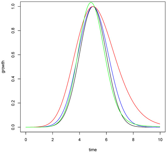
Figure 1. Curves related to the direct problem for a fractional Gaussian model.

In the same direction, the following observation equation is associated with the model

$$y_i=g(f(x_i))+\epsilon ,i=1,\dots ,n$$

(12)

where $y_i$ corresponds to the i-th observed value under uncertainty from a solution of Equation (4) associated with the direct problem on the alcohol concentration in blood at the discrete times $t_i\in [0;T];i=1,2,\dots ,n$; g is the observation function and ${ϵ}_i$ are measurement errors, which are considered as independent and identically distributed (i.i.d.) random variables from a normal distribution, with mean zero and constant variance ${\sigma }^2$, denoted by ${\epsilon }_i\sim \mathcal{N}(0,{\sigma }^2)$.

3. Estimation for Comformable Gaussian Models

In Equations (4) and (12), the parameter of interest is $\varphi =(a,b,c,\alpha ,{\sigma }^2)$. The prior distributions used are: $a\sim \mathcal{G}({\gamma }_a,{\mu }_a)$, $b\sim \mathcal{G}({\gamma }_b,{\mu }_b)$, $c\sim \mathcal{G}({\gamma }_c,{\mu }_c)$, and $\tau \sim \mathcal{G}({\gamma }_{\tau },{\mu }_{\tau })$, where $\mathcal{G}(\gamma ,\mu )$ denotes the Gamma distribution with shape parameter $\gamma$ and rate parameter $\mu$, where $\alpha \sim \mathcal{U}(0,1)$, $\tau =1/{\sigma }^2.$ $\mathcal{U}$ is the continuous Uniform distribution on the interval $(0,1)$. Based on our knowledge, the same a priori distributions associated with the parameters of interest of the different fractional models were chosen, with the objective of evaluating their behaviour under equal conditions. Note that different a priori distributions produce different a posteriori distributions of the parameters, and the estimated values will be subject to the permissible values of that distribution.

In (4), $a>0$ and $\alpha \in (0,1]$, the join prior distribution is represented as: $p(\varphi |hyperparameters)=p(a|{\gamma }_a,{\mu }_a)p(b|{\gamma }_b,{\mu }_b)p(c|{\gamma }_c,{\mu }_c)p(\alpha )p(\tau |{\gamma }_{\tau },{\mu }_{\tau })$, where $p(a|{\gamma }_a,{\mu }_a)$, $p(b|{\gamma }_b,{\mu }_b)$, $p(c|{\gamma }_c,{\mu }_c)$, $p(\alpha )$ and $p(\tau |{\gamma }_{\tau },{\mu }_{\tau })$ have been previously defined.

Let $O^{\prime }=(O_1,O_2,\dots ,O_n)$ denote observed data at times, which are independent and identically distributed $(t_1,t_2,\dots ,t_n)$ from the Equations (4) and (12); the likelihood function is:

$$\begin{array}{c}\hfill L(O|\varphi )=\prod _{i=1}^n{f}_O(O_i)=\frac{1}{{(\sigma \sqrt{2\pi })}^n}exp\left\{-\frac{1}{2{\sigma }^2}\sum _{i=1}^n{(O_i-g(y(t_i)))}^2\right\},\end{array}$$

(13)

where $y(t_i),i=1,\dots ,n$ is a solution of Equation (4).

The posterior distribution is given by

$$\begin{array}{c}\hfill p(\varphi |O)=\frac{L(O|\varphi )p(\varphi )}{{\int }_{\ominus }L(O|\varphi )p(\varphi )d\varphi },\end{array}$$

(14)

where ⊖ denotes the parameter space of $\varphi$. It is known that

$$\begin{array}{c}\hfill p(\varphi |O)\propto L(O|\varphi )p(\varphi ).\end{array}$$

(15)

Assuming a loss quadratic function, the Bayesian point estimation is the posterior mean of ${\widehat{\varphi }}_B$, which is given by ${\widehat{\varphi }}_B=E(\varphi |O)$.

For this study, statistical and computational methods developed in the following works were used [23,24,25,26,27,28,29,30,31].

In this part, we analyze two applications with real and simulated data of the Gaussian model through the following approaches: Khalil’s operator (blue), conformable derivative with $T(t,\alpha )=e^{(1-\alpha )t}$ (red), Grünwald–Letnikov derivative (green), and ordinary derivative (black).

The real data on the alcohol concentration in blood appear in [32]. The adjustments corresponding to the observations (black line) associated with the alcohol concentration in blood are shown in Figure 2.

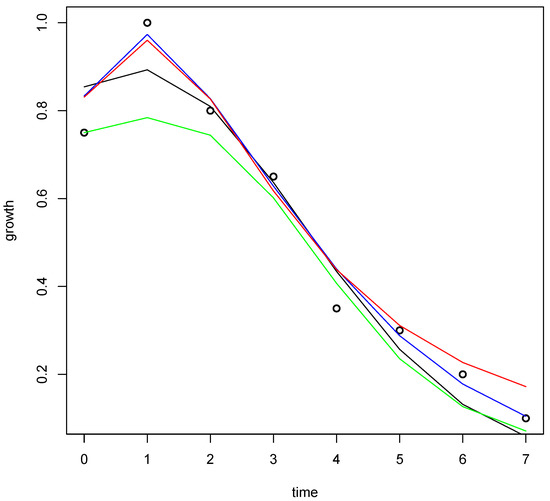
Figure 2. Data and estimates of the alcohol concentration in blood.

The ${\ell }^2$-errors related to the approaches are: Khalil’s derivative (0.01756749), $G_T^{\alpha }$ with $T(t,\alpha )=e^{(\alpha -1)t}$ (0.02370243), Grünwald–Letnikov derivative (0.06573368) and ordinary derivative (0.03790216).

Figure 3 shows the trace and estimated posterior distributions of the parameters of interest using Khalil’s derivatives.

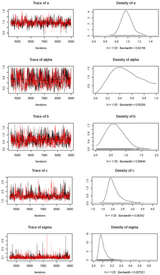
Figure 3. Trace and estimated posterior densities of $\alpha$, a, b, c, and $\sigma$.

The adjustments corresponding to the observations (black points) associated with simulated data are shown in Figure 4. The ${\ell }^2$-errors related to the approaches are: Khalil’s derivative (0.12640866), $G_T^{\alpha }$ with $T(t,\alpha )=e^{(\alpha -1)t}$ (0.01563364), Grünwald–Letnikov derivative (1.74848946), and ordinary derivative (0.52879824).

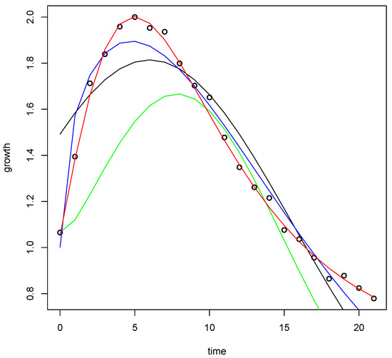
Figure 4. Data and estimates of simulated data.

Figure 5 shows the trace and estimated posterior distributions of the parameters of interest using $G_T^{\alpha }$ with $T(t,\alpha )=e^{(1-\alpha )t}$) fracional derivatives.

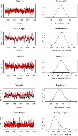
Figure 5. Trace and estimated posterior densities of $\alpha$, a, b, c, and $\sigma$.

4. Conclusions

In this paper, we used a generalized conformable derivative ($G_T^{\alpha }$ with $T(t,\alpha )=e^{(1-\alpha )t}$), $T(t,\alpha )=t^{(1-\alpha )t}$), Grünwald–Letnikov fractional derivatives and clasical derivatives in order to study a fractional Gaussian model associated with the alcohol level in blood. Taking into account an experimental dataset, we solve an inverse problem to estimate the order $\alpha$ of the involved fractional derivative.

The estimates of $\alpha$, a, b, c, and $\tau$ related to the data of alcohol concentration in blood are: related to the data of alcohol concentration in blood are shown in Table 1:

Table 1. Parameter estimates related to blood alcohol concentration data.

Derivative	$\mathit{\alpha }$	a	b	c	$\mathit{\tau }$
Ordinary	$-$	0.8951823	0.8119931	2.6501296	0.1195180
$G_T^{\alpha }$; $T(t,\alpha )=e^{(1-\alpha )t}$	0.6728009	0.9622524	0.8831519	1.5542520	0.1033001
Khalil et al.	0.4848604	0.9894414	0.6424266	2.0477500	0.0974800
Grünwald–Letnikov	0.7027876	-	1.7451992	2.2566254	0.1232454

This work shows that a better data fit is accomplished when using fractional derivatives. The use of the conformable derivative $G_T^{\alpha }$ with a generic $T(t,\alpha )$ guarantees a best curve fit when a specific kernel is used for each data set type.

References

- Podlubny, I. Fractional Differential Equations; Academic Press: Athens, OH, USA, 1999. [Google Scholar]
- Abel, N.H. Solution de quelques problemes a láide d’intégrales définieas. Oeuvres complétes. Christiania (Grondahl) 1881, 1, 11–27. [Google Scholar]
- Monje, C.A.; Chen, Y.; Vinagre, B.M.; Xue, D.; Feliu-Batlle, V. Fractional-Order Systems and Controls: Fundamentals and Applications; Springer Science and Business Media: London, UK, 2010. [Google Scholar]
- Vazquez, L.; Trujillo, J.; Velasco, M.P. Fractional heat equation and the second law of thermodynamics. Fract. Calc. Appl. Anal. 2011, 14, 334–342. [Google Scholar] [CrossRef]
- Area, I.; Batarfi, H.; Losada, J.; Nieto, J.J.; Shammakh, W.; Torres, A. On a fractional order Ebola epidemic model. Adv. Differ. Equ. 2015, 2015, 278. [Google Scholar] [CrossRef]
- Santiesteban, T.R.G.; Blaya, R.A.; Reyes, J.B.; Sigarreta, J.M. A Cauchy transform for polyanalytic functions on fractal domains. Ann. Pol. Math. 2018, 121, 21–32. [Google Scholar] [CrossRef]
- Ortega, A.; Rosales, J.J. Newton’s law of cooling with fractional conformable derivative. Rev. Mex. Fis. 2018, 64, 172. [Google Scholar] [CrossRef]
- Lei, G.; Cao, N.; Liu, D.; Wang, H. A nonlinear flow model for porous media based on conformable derivative approach. Energies 2018, 11, 2986. [Google Scholar] [CrossRef]
- Khalil, R.; Al Horani, M.; Yousef, A.; Sababheh, M. A new definition of fractional derivative. J. Comput. Appl. Math. 2014, 264, 65–70. [Google Scholar] [CrossRef]
- Katugampola, U.N. A new fractional derivative with classical properties. arXiv 2014, arXiv:1410.6535. [Google Scholar]
- Almeida, R.; Guzowska, M.; Odzijewicz, T. A remark on local fractional calculus and ordinary derivatives. Open Math. 2016, 14, 1122–1124. [Google Scholar] [CrossRef]
- Sousa, J.V.D.C.; de Oliveira, E.C. A new truncated M-fractional derivative type unifying some fractional derivative types with classical properties. arXiv 2017, arXiv:1704.08187. [Google Scholar]
- Guzman, P.M.; Langton, G.; Lugo, L.M.; Medina, J.; Nápoles, J.E. A new definition of a fractional derivative of local type. J. Math. Anal. 2018, 9, 88–98. [Google Scholar]
- Nápoles, J.E.; Rodríguez, J.M.; Sigarreta, J.M. New Hermite–Hadamard Type Inequalities Involving Non-Conformable Integral Operators. Symmetry 2019, 11, 1108. [Google Scholar] [CrossRef]
- Fleitas, A.; Nápoles, J.E.; Rodríguez, J.M.; Sigarreta, J.M. Note on the generalized conformable derivative. 2019. submited. [Google Scholar]
- Almeida, R.; Bastos, N.R.; Monteiro, M.T. Modeling some real phenomena by fractional differential equations. Math. Meth. Appl. Sci. 2016, 39, 4846–4855. [Google Scholar] [CrossRef]
- Kanth, A.R.; Garg, N. Computational Simulations for Solving a Class of Fractional Models via Caputo-Fabrizio Fractional Derivative. Proc. Comp. Sci. 2018, 125, 476–482. [Google Scholar] [CrossRef]
- Caputo, M.; Fabrizio, M. A new definition of fractional derivative without singular kernel. Progr. Fract. Differ. Appl. 2015, 1, 1–13. [Google Scholar]
- Qureshi, S.; Yusuf, A.; Shaikh, A.; Inc, A.; Baleanu, D. Fractional modeling of blood ethanol concentration system with real data application. Chaos 2019, 29, 013143. [Google Scholar] [CrossRef]
- Saad, K.M.; Baleanu, D.; Atangana, A. New fractional derivatives applied to the Korteweg—de Vries and Korteweg—de Vries—Burgers’ equations. Comput. Appl. Math. 2018, 37, 5203–5216. [Google Scholar] [CrossRef]
- Abdejjawad, T. On conformable fractional calculus. J. Comput. Appl. Math. 2015, 279, 57–66. [Google Scholar] [CrossRef]
- Jarad, F.; Ugurlu, E.; Abdeljawad, T.; Baleanu, D. On a new class of fractional operators. Adv. Differ. Equ. 2017, 247. [Google Scholar] [CrossRef]
- Gelfand, A.E.; Smith, A.F.M. Sampling-based approaches to calculating marginal densities. J. Am. Statist. Assoc. 1990, 85, 398–409. [Google Scholar] [CrossRef]
- Metropolis, N.; Rosenbluth, A.W.; Rosenbluth, M.N.; Teller, A.H.; Teller, E. Equation of state calculations by fast computing machines. J. Chem. Phys. 1953, 21, 1087–1092. [Google Scholar] [CrossRef]
- Plummer, M. JAGS: A program for analysis of Bayesian graphical models using Gibbs sampling. In Proceedings of the 3rd International Workshop on Distributed Statistical Computing, Vienna, Austria, 20–22 March 2003; p. 10. [Google Scholar]
- Christen, J.A.; Fox, C.; Pérez Ruiz, A.; Santana Cibrian, M. On optimal direction gibbs sampling. Available online: https://arxiv.org/abs/1205.4062 (accessed on 18 May 2012).
- R Core Team. R: A Language and Environment for Statistical Computing; R Core Team: Vienna, Austria, 2013; p. 201. [Google Scholar]
- Su, Y.S.; Yajima, M. R2jags: A Package for Running jags from R. R package version 0.03-08. 2012. Available online: http://CRAN.R-project.org/package=R2jags (accessed on 18 May 2012).
- Plummer, M. Bayesian graphical models using MCMC. R package version 3-13. Retrieved November 2014, 10, 2015. [Google Scholar]
- Neal, R.M. Slice sampling. Ann. Statist. 2003, 31, 705–767. [Google Scholar] [CrossRef]
- Gilks, W.R.; Wild, P. Adaptive rejection sampling for Gibbs sampling. J. R. Stat. Soc. Ser. C (Appl. Statist.) 1992, 41, 337–348. [Google Scholar] [CrossRef]
- Ludwin, C. Blood alcohol content. UJMM: One+ Two 2011, 3, 1. [Google Scholar] [CrossRef][Green Version]
© 2020 by the authors. Licensee MDPI, Basel, Switzerland. This article is an open access article distributed under the terms and conditions of the Creative Commons Attribution (CC BY) license (http://creativecommons.org/licenses/by/4.0/).