Finite-Time Control for Nonlinear Systems with Time-Varying Delay and Exogenous Disturbance

Abstract

This paper is concerned with the problem of finite-time control for nonlinear systems with time-varying delay and exogenous disturbance, which can be represented by a Takagi–Sugeno (T-S) fuzzy model. First, by constructing a novel augmented Lyapunov–Krasovskii functional involving several symmetric positive definite matrices, a new delay-dependent finite-time boundedness criterion is established for the considered T-S fuzzy time-delay system by employing an improved reciprocally convex combination inequality. Then, a memory state feedback controller is designed to guarantee the finite-time boundness of the closed-loop T-S fuzzy time-delay system, which is in the framework of linear matrix inequalities (LMIs). Finally, the effectiveness and merits of the proposed results are shown by a numerical example.

1. Introduction

During the past several decades, the control problem of nonlinear systems has attracted considerable attention [1,2,3,4,5,6] as various practical systems are essentially nonlinear and cannot be easily simplified into a linear model. Up to now, many fuzzy logic control approaches have been proposed for the control problem of nonlinear systems. In particular, the Takagi–Sugeno (T-S) fuzzy model, developed in [7], is an important tool to approximate complex nonlinear systems by combining the fruitful linear system theory and the flexible fuzzy logic approach. Additionally, time-delay is unavoidably encountered in many dynamic systems, such as power systems, network control systems, neural networks, etc., which often results in chaos, oscillation, and even instability. Therefore, the study of T-S fuzzy time-delay systems has become more and more popular in recent years. In particular, many significant and interesting results on stability analysis and the control synthesis of T-S fuzzy time-delay systems have been developed in the literature [8,9,10,11,12,13,14,15].

Much attention has been paid to obtain the delay-dependent stability criteria for T-S fuzzy time-delay systems over the last few decades. It is well-known that the conservativeness of the stability criteria mainly has two sources: the choice of the Lyapunov–Krasovskii functional (LKF) and the estimation of its derivative. It is of great importance to construct an appropriate Lyapunov–Krasovskii functional for deriving less conservative stability conditions. In recent years, delay-partitioning Lyapunov–Krasovskii functionals and augmented Lyapunov–Krasovskii functionals have been developed to reduce the conservativeness of simple LKFs and have attracted growing attention. A delay-partitioning approach was applied to study the Lyapunov asymptotic stability of T-S fuzzy time-delay systems and some less conservative stability conditions were obtained in [16,17,18].

In [19], the authors introduced the triple-integral terms into the LKFs to derive the stability conditions for T-S fuzzy time-delay systems. In addition, various approaches have been proposed to estimate the derivatives of LKFs when dealing with stability analysis and control synthesis of time-delay systems, such as the free weighting matrix approach [20], Jensen inequality approach [21], Wirtinger-based integral inequality approach [10], reciprocally convex combination approach [22], auxiliary function-based inequality approach [23], and free-matrix-based integral inequality approach [24].

By applying the Wirtinger-based integral inequality approach and reciprocally convex combination approach, Zeng et al. [18] derived some less conservative stability criteria for uncertain T-S fuzzy systems with time-varying delays. An improved free weighting matrix approach was employed to obtain several new delay-dependent stability conditions in terms of the linear matrix inequalities for T-S fuzzy systems with time-varying delays in [25]. In [26], the authors investigated Lyapunov asymptotic stability analysis problems for T-S fuzzy time-delay systems by constructing a new augmented Lyapunov–Krasovskii functional and employing the free-matrix-based integral inequality approach.

The aforementioned results regarding the stability analysis of T-S fuzzy systems mainly focus on Lyapunov asymptotic stability, in which the states of systems converge asymptotically to equilibrium in an infinite time interval. However, in many practical engineering applications, the main concern may be the transient performances of the system trajectory during a specified finite-time interval. Unlike Lyapunov asymptotic stability, finite-time stability, introduced in [27], is another stability concept, which requires that the states of dynamical systems do not exceed a certain threshold in a fixed finite-time interval with a given bound for the initial condition. Up to now, the problem of finite-time stability, finite-time boundedness, and finite-time stabilization of dynamical systems has attracted growing attention, and many significant results have been reported in [28,29,30,31,32].

Several results on finite-time stability and stabilization of T-S fuzzy systems can also be found. The problem of finite-time stability and finite-time stabilization for T-S fuzzy time-delay systems was investigated in [28]. Sakthivel et al. [31] studied finite-time dissipative based fault-tolerant control problem for a class of T-S fuzzy systems with a constant delay. However, to the best of our knowledge, until now there have been few results on finite-time boundedness and finite-time stabilization of T-S fuzzy systems with time-varying delay and exogenous disturbance. Furthermore, it should be mentioned that most of the existing works on finite-time control for T-S fuzzy time-delay systems are fairly conservative. Motivated by the above discussions, in this paper, we deal with the problem of finite-time control for a class of nonlinear systems with time-varying delay and exogenous disturbance, which can be described by a T-S fuzzy model.

The main contributions of this paper are summarized as follows. First, a new augmented Lyapunov–Krasovskii functional is constructed, which makes full use of the information about time-varying delay. Based on the proposed Lyapunov–Krasovskii functional, a less conservative finite-time boundedness condition is obtained for T-S fuzzy time-delay systems by utilizing an improved reciprocally convex combination technique. Second, based on parallel distributed compensation schemes, a memory state feedback controller is designed to finite-time stabilize the T-S fuzzy time-delay system, which can be derived by solving a series of linear matrix inequalities (LMIs). Finally, a numerical example is given to illustrate the advantages and validity of the developed results.

The rest of this paper is organized as follows: the problem statement is given in Section 2. The main results on the finite-time boundedness and finite-time stabilization of nonlinear systems with time-varying delay and exogenous disturbance are presented in Section 3. In Section 4, a numerical example is proposed to show the effectiveness of the developed results. Finally, our conclusions are drawn in Section 5.

Notations: Throughout this paper, ${\mathbf{R}}^n$ denotes the n-dimensional Euclidean space; ${\mathbf{R}}^{n\times m}$ stands for the set of all $n\times m$ real matrices; the superscripts T and $-1$ denote the transpose and inverse of a matrix, respectively; I and 0 represent the identity matrix and zero matrix, respectively, with compatible dimensions; $diag\{\cdots \}$ denotes a block-diagonal matrix; the notation $P>0(\ge 0)$ means that the matrix P is real symmetric and positive definite (semi-positive definite); ∗ stands for the symmetric terms in a symmetric matrix; for any matrix $X\in {\mathbf{R}}^{n\times n}$, $Sym\left\{X\right\}$ is defined as $X+X^T$.

2. Problem Formulation

Consider a class of nonlinear systems with time-varying delay and exogenous disturbance, which can be represented by the following T-S fuzzy model:

Plant Rule i:

IF ${\xi }_1\left(t\right)$ is $N_{i1}$, ⋯, and ${\xi }_p\left(t\right)$ is $N_{ip}$,

THEN

$$\left\{\begin{array}{c}\dot{x}\left(t\right)=A_{i}x\left(t\right)+A_{di}x(t-d\left(t\right))+B_{i}u\left(t\right)+G_i\omega \left(t\right)\hfill \\ x\left(t\right)=\varphi \left(t\right),\hspace{1em}t\in [-h,0]\hfill \end{array}\right.$$

where $i\in \{1,2,\dots ,r\}$, r is the number of IF-THEN rules, $x\left(t\right)\in {\mathbf{R}}^n$ is the state vector, $u\left(t\right)\in {\mathbf{R}}^p$ is the control input, $\omega \left(t\right)\in {\mathbf{R}}^l$ is the exogenous disturbance, which satisfies ${\int }_0^{T_f}\omega {\left(t\right)}^T\omega \left(t\right)dt\le \delta$; $\delta \ge 0$ is a given scalar. $A_i$, $A_{di}$, $B_i$, and $G_i$ are known constant matrices with appropriate dimensions. ${\xi }_1\left(t\right),{\xi }_2\left(t\right),\dots ,{\xi }_p\left(t\right)$ are premise variables, $N_{i1},N_{i2},\dots ,N_{ip}$ are fuzzy sets. The time delay $d\left(t\right)$ is a time-varying function that satisfies

$$\begin{array}{c}\hfill 0\le d\left(t\right)\le h\hspace{1em}and\hspace{1em}{\mu }_1\le \dot{d}\left(t\right)\le {\mu }_2\end{array}$$

(1)

where $h>0$ and ${\mu }_1,{\mu }_2$ are constants. The initial condition $\varphi \left(t\right)$ is a continuous vector-valued function for all $t\in [-h,0]$.

Let $\xi \left(t\right)={[{\xi }_1\left(t\right),{\xi }_2\left(t\right),\dots ,{\xi }_p\left(t\right)]}^T$, by employing a singleton fuzzifier, product inference, and center-average defuzzifer, the input–output form of the above T-S fuzzy time-delay system can be represented by

$$\begin{array}{c}\hfill \dot{x}\left(t\right)=\sum _{i=1}^r{\rho }_i\left(\xi \left(t\right)\right)\{A_{i}x\left(t\right)+A_{di}x(t-d\left(t\right))+B_{i}u\left(t\right)+G_i\omega \left(t\right)\}\end{array}$$

(2)

where ${\rho }_i\left(\xi \left(t\right)\right)=\frac{{\theta }_i\left(\xi \left(t\right)\right)}{{\sum }_{i=1}^r{\theta }_i\left(\xi \left(t\right)\right)}$, ${\theta }_i\left(\xi \left(t\right)\right)={\prod }_{j=1}^p{N}_{ij}\left({\xi }_j\left(t\right)\right)$, $N_{ij}\left({\xi }_j\left(t\right)\right)$ is the grade of membership of ${\xi }_j\left(t\right)$ in the fuzzy set $N_{ij}$. We note that ${\theta }_i\left(\xi \left(t\right)\right)\ge 0$, ${\sum }_{i=1}^r{\theta }_i\left(\xi \left(t\right)\right)>0$ for all t, and we can obtain ${\rho }_i\left(\xi \left(t\right)\right)\ge 0$, ${\sum }_{i=1}^r{\rho }_i\left(\xi \left(t\right)\right)=1$.

In this paper, for simplicity, we denote $S\left(t\right)={\sum }_{i=1}^r{\rho }_i\left(\xi \left(t\right)\right)S_i$ for any matrix $S_i$. Therefore, the T-S fuzzy time-delay system (2) can be rewritten as follows:

$$\begin{array}{c}\hfill \dot{x}\left(t\right)=A\left(t\right)x\left(t\right)+A_d\left(t\right)x(t-d\left(t\right))+B\left(t\right)u\left(t\right)+G\left(t\right)\omega \left(t\right).\end{array}$$

(3)

Now, the definition of finite-time boundedness (FTB) for the T-S fuzzy time-delay system (3) with $u\left(t\right)\equiv 0$ is given as follows:

Definition 1

([31]). The T-S fuzzy time-delay system (3) with $u\left(t\right)\equiv 0$ is said to be finite-time bounded with respect to $(c_1,c_2,T_f,R,\delta ,h)$, where $0<c_1<c_2$, $T_f>0$, $R\in$ ${\mathit{R}}^{n\times n}$ and $R>0$, if

$$\begin{array}{c}\hfill su{p}_{-h\le \theta \le 0}\{x^T\left(\theta \right)Rx\left(\theta \right),{\dot{x}}^T\left(\theta \right)R\dot{x}\left(\theta \right)\}\le c_1\Rightarrow x^T\left(t\right)Rx\left(t\right)<c_2,\end{array}$$

$\forall t\in [0,T_f],\forall \omega \left(t\right):{\int }_0^{T_f}\omega {\left(t\right)}^T\omega \left(t\right)dt\le \delta$.

Based on the parallel distributed compensation scheme, we aim to design the following memory state feedback controller, which can guarantee the corresponding closed-loop T-S fuzzy time-delay system finite-time bounded:

$$\begin{array}{c}\hfill u\left(t\right)=K_1\left(t\right)x\left(t\right)+K_2\left(t\right)x(t-d\left(t\right)),\end{array}$$

(4)

where $K_1\left(t\right)={\sum }_{j=1}^r{\rho }_j\left(\xi \left(t\right)\right)K_{1j}$, $K_2\left(t\right)={\sum }_{j=1}^r{\rho }_j\left(\xi \left(t\right)\right)K_{2j}$, and $K_{1j},K_{2j},j=1,2,\dots ,r$ are the state feedback gain matrices to be determined.

By substituting (4) into (3), the corresponding closed-loop T-S fuzzy time-delay system can be represented as follows:

$$\begin{array}{c}\hfill \dot{x}\left(t\right)=[A\left(t\right)+B\left(t\right)K_1\left(t\right)]x\left(t\right)+[A_d\left(t\right)+B\left(t\right)K_2\left(t\right)]x(t-d\left(t\right))+G\left(t\right)\omega \left(t\right).\end{array}$$

(5)

In order to derive the main results in this paper, the following lemma, i.e., the improved reciprocally convex combination inequality approach will be utilized in finite-time boundedness analysis and controller design of T-S fuzzy time-delay systems.

Lemma 1

([33]). Let $R_1,R_2\in {\mathit{R}}^{m\times m}$ be real symmetric positive definite matrices, ${\varpi }_1,{\varpi }_2\in {\mathit{R}}^m$ and a scalar $\alpha \in (0,1)$. Then for any matrices $Y_1,Y_2\in {\mathit{R}}^{m\times m}$, the following inequality holds

$$\begin{array}{cc}& \frac{1}{\alpha }{\varpi }_1^T{R}_1{\varpi }_1+\frac{1}{1-\alpha }{\varpi }_2^T{R}_2{\varpi }_2\hfill \\ \hfill \ge & {\varpi }_1^T[R_1+(1-\alpha )(R_1-Y_1{R}_2^{-1}{Y}_1^T)]{\varpi }_1\hfill \\ & + {\varpi }_2^T[R_2+\alpha (R_2-Y_2^T{R}_1^{-1}{Y}_2)]{\varpi }_2\hfill \\ & + 2{\varpi }_1^T[\alpha Y_1+(1-\alpha )Y_2]{\varpi }_2.\hfill \end{array}$$

3. Main Results

3.1. Finite-Time Boundedness Analysis

In this subsection, our aim is to develop a new delay-dependent finite-time boundedness criterion for T-S fuzzy systems with time-varying delay and norm-bounded disturbance. Before deriving the main results, the nomenclature simplifying the representations for matrices and vectors is given as follows:

$$\begin{array}{c}\hfill {\epsilon }_1\left(t\right)=\left(\begin{array}{c}x\left(t\right)\\ x(t-d(t\left)\right)\\ x(t-h)\\ \dot{x}(t-d\left(t\right))\\ \dot{x}(t-h)\end{array}\right),\hspace{1em}{\epsilon }_2\left(t\right)=\left(\begin{array}{c}\frac{1}{d\left(t\right)}{\int }_{t-d\left(t\right)}^{t}x\left(s\right)ds\\ \frac{1}{h-d\left(t\right)}{\int }_{t-h}^{t-d\left(t\right)}x\left(s\right)ds\\ \frac{1}{d^2\left(t\right)}{\int }_{t-d\left(t\right)}^t{\int }_{\theta }^{t}x\left(s\right)dsd\theta \\ \frac{1}{{\left(h-d\left(t\right)\right)}^2}{\int }_{t-h}^{t-d\left(t\right)}{\int }_{\theta }^{t-d\left(t\right)}x\left(s\right)dsd\theta \\ \frac{1}{h}{\int }_{t-h}^{t}x\left(s\right)ds\\ \frac{1}{h^2}{\int }_{t-h}^t{\int }_{\theta }^{t}x\left(s\right)dsd\theta \\ \omega \left(t\right)\end{array}\right),\end{array}$$

$$\begin{array}{c}\hfill \epsilon \left(t\right)={\left[{\epsilon }_1^T\left(t\right)\hspace{1em}{\epsilon }_2^T\left(t\right)\right]}^T,\hspace{1em}\tilde{\epsilon }\left(t\right)={\left[{\epsilon }_1^T\left(t\right)\hspace{1em}{\epsilon }_2^T\left(t\right)\hspace{1em}{\dot{x}}^T\left(t\right)\right]}^T,\end{array}$$

$$\begin{array}{c}\hfill e_i=\left[0_{n\times \left(i-1\right)n}\hspace{1em}{I}_n\hspace{1em}{0}_{n\times \left(12-i\right)n}\right],\hspace{1em}i=1,2,\cdots ,12,\end{array}$$

$$\begin{array}{c}\hfill {\tilde{e}}_i=\left[0_{n\times \left(i-1\right)n}\hspace{1em}{I}_n\hspace{1em}{0}_{n\times \left(13-i\right)n}\right],\hspace{1em}i=1,2,\cdots ,13.\end{array}$$

Theorem 1.

For given scalars $h>0$ and ${\mu }_1,{\mu }_2$, the T-S fuzzy system (3) with $u\left(t\right)=0$ and a time-varying delay $d\left(t\right)$ satisfying (1) is finite-time bounded with respect to $(c_1,c_2,T_f,R,\delta ,h)$, if there exists a scalar $\beta >0$, symmetric positive definite matrices $P\in {\mathit{R}}^{5n\times 5n}$, $S_1,S_2\in {\mathit{R}}^{2n\times 2n}$, $Q_1,Q_2\in {\mathit{R}}^{3n\times 3n}$, $W,Z,U\in {\mathit{R}}^{n\times n}$, and any matrices $Y_1,Y_2\in {\mathit{R}}^{3n\times 3n}$, such that the following conditions hold:

$$\begin{array}{c}\hfill \left(\begin{array}{cc}{\mathsf{\Sigma }}_{1i}(0,{\mu }_1)& {\mathsf{\Lambda }}_1^T{Y}_1\\ Y_1^T{\mathsf{\Lambda }}_1& -W_0\end{array}\right)<0,\hspace{1em}i=1,2,\dots ,r\end{array}$$

(6)

$$\begin{array}{c}\hfill \left(\begin{array}{cc}{\mathsf{\Sigma }}_{1i}(0,{\mu }_2)& {\mathsf{\Lambda }}_1^T{Y}_1\\ Y_1^T{\mathsf{\Lambda }}_1& -W_0\end{array}\right)<0,\hspace{1em}i=1,2,\dots ,r\end{array}$$

(7)

$$\begin{array}{c}\hfill \left(\begin{array}{cc}{\mathsf{\Sigma }}_{1i}(h,{\mu }_1)& {\mathsf{\Lambda }}_2^T{Y}_2^T\\ Y_2{\mathsf{\Lambda }}_2& -W_0\end{array}\right)<0,\hspace{1em}i=1,2,\dots ,r\end{array}$$

(8)

$$\begin{array}{c}\hfill \left(\begin{array}{cc}{\mathsf{\Sigma }}_{1i}(h,{\mu }_2)& {\mathsf{\Lambda }}_2^T{Y}_2^T\\ Y_2{\mathsf{\Lambda }}_2& -W_0\end{array}\right)<0,\hspace{1em}i=1,2,\dots ,r\end{array}$$

(9)

$$\begin{array}{c}\hfill c_1\mathsf{\Pi }+{\lambda }_{37}\delta <{\lambda }_{36}{c}_2{e}^{-\beta T_f},\end{array}$$

(10)

where

$$\begin{array}{ccc}\hfill P& =& \left(\begin{array}{ccccc}{P}_{11}& P_{12}& P_{13}& P_{14}& P_{15}\\ \ast & P_{22}& P_{23}& P_{24}& P_{25}\\ \ast & \ast & P_{33}& P_{34}& P_{35}\\ \ast & \ast & \ast & P_{44}& P_{45}\\ \ast & \ast & \ast & \ast & P_{55}\end{array}\right),\hspace{1em}{Q}_1=\left(\begin{array}{ccc}{Q}_{11}& Q_{12}& Q_{13}\\ \ast & Q_{22}& Q_{23}\\ \ast & \ast & Q_{33}\end{array}\right),\hspace{1em}{Q}_2=\left(\begin{array}{ccc}{q}_{11}& q_{12}& q_{13}\\ \ast & q_{22}& q_{23}\\ \ast & \ast & q_{33}\end{array}\right),\hfill \\ \hfill S_1& =& \left(\begin{array}{cc}{S}_{11}& S_{12}\\ \ast & S_{22}\end{array}\right),\hspace{1em}{S}_2=\left(\begin{array}{cc}{s}_{11}& s_{12}\\ \ast & s_{22}\end{array}\right),\hfill \end{array}$$

$$\begin{array}{cc}\hfill {\mathsf{\Sigma }}_{1i}(d\left(t\right),\dot{d}\left(t\right))=& Sym\left\{{\mathsf{\Xi }}_1^{T}P{\mathsf{\Xi }}_{2i}\right\}+\dot{d}\left(t\right){\mathsf{\Xi }}_3^T{S}_1{\mathsf{\Xi }}_3-\dot{d}\left(t\right){\mathsf{\Xi }}_4^T{S}_2{\mathsf{\Xi }}_4+Sym({\mathsf{\Xi }}_3^T{S}_1{\mathsf{\Xi }}_{5i}+{\mathsf{\Xi }}_4^T{S}_2{\mathsf{\Xi }}_{6i})\hfill \\ & +Sym\left({\mathsf{\Xi }}_7^T{Q}_1{\mathsf{\Xi }}_{8i}\right)+{\mathsf{\Xi }}_{9i}^T{Q}_1{\mathsf{\Xi }}_{9i}-(1-\dot{d}\left(t\right)){\mathsf{\Xi }}_{10}^T{Q}_1{\mathsf{\Xi }}_{10}+Sym\left({\mathsf{\Xi }}_{11}^T{Q}_2{\mathsf{\Xi }}_{12}\right)\hfill \\ & +(1-\dot{d}\left(t\right)){\mathsf{\Xi }}_{13}^T{Q}_2{\mathsf{\Xi }}_{13}-{\mathsf{\Xi }}_{14}^T{Q}_2{\mathsf{\Xi }}_{14}+h^2{e}_{si}^{T}W{e}_{si}+\frac{h^4}{4}{e}_{si}^{T}Z{e}_{si}-h^2{\mathsf{\Xi }}_{15}^{T}Z{\mathsf{\Xi }}_{15}\hfill \\ & -2h^2{\mathsf{\Xi }}_{16}^{T}Z{\mathsf{\Xi }}_{16}-e_{12}^{T}U{e}_{12}+(\alpha -2){\mathsf{\Lambda }}_1^T{W}_0{\mathsf{\Lambda }}_1-(\alpha +1){\mathsf{\Lambda }}_2^T{W}_0{\mathsf{\Lambda }}_2\hfill \\ & -Sym\left\{{\mathsf{\Lambda }}_1^T[\alpha Y_1+(1-\alpha )Y_2]{\mathsf{\Lambda }}_2\right\},\hfill \end{array}$$

$$\begin{array}{ccc}\hfill \alpha & =& \frac{d\left(t\right)}{h},\hspace{1em}\hspace{1em}\hspace{1em}{W}_0=diag\{W,3W,5W\},\hspace{1em}\hspace{1em}\hspace{1em}{\mathsf{\Xi }}_1={\left[e_1^T\hspace{1em}{e}_2^T\hspace{1em}{e}_3^T\hspace{1em}d\left(t\right)e_6^T\hspace{1em}(h-d\left(t\right))e_7^T\right]}^T,\hfill \\ \hfill {\mathsf{\Xi }}_{2i}& =& {[e_{si}^T\hspace{1em}(1-\dot{d}\left(t\right))e_4^T\hspace{1em}{e}_5^T\hspace{1em}{e}_1^T-(1-\dot{d}\left(t\right))e_2^T\hspace{1em}(1-\dot{d}\left(t\right))e_2^T-e_3^T]}^T,\hfill \\ \hfill {\mathsf{\Xi }}_3& =& {\left[e_1^T\hspace{1em}{e}_6^T\right]}^T,\hspace{1em}\hspace{1em}\hspace{1em}{\mathsf{\Xi }}_4={\left[e_1^T\hspace{1em}{e}_7^T\right]}^T,\hspace{1em}\hspace{1em}\hspace{1em}{\mathsf{\Xi }}_{5i}={\left[d\left(t\right)e_{si}^T\hspace{1em}-\dot{d}\left(t\right)e_6^T+e_1^T-(1-\dot{d}\left(t\right))e_2^T\right]}^T,\hfill \\ \hfill {\mathsf{\Xi }}_{6i}& =& {\left[(h-d\left(t\right))e_{si}^T\hspace{1em}\dot{d}\left(t\right)e_7^T+(1-\dot{d}\left(t\right))e_2^T-e_3^T\right]}^T,\hspace{1em}{\mathsf{\Xi }}_7={\left[d\left(t\right)e_6^T\hspace{1em}{e}_1^T-e_2^T\hspace{1em}d\left(t\right)(e_1^T-e_6^T)\right]}^T,\hfill \\ \hfill {\mathsf{\Xi }}_{8i}& =& {\left[0\hspace{1em}0\hspace{1em}{e}_{si}^T\right]}^T,\hspace{1em}{\mathsf{\Xi }}_{9i}={\left[e_1^T\hspace{1em}{e}_{si}^T\hspace{1em}0\right]}^T,\hspace{1em}{\mathsf{\Xi }}_{10}={\left[e_2^T\hspace{1em}{e}_4^T\hspace{1em}{e}_1^T-e_2^T\right]}^T,\hfill \\ \hfill {\mathsf{\Xi }}_{11}& =& {[(h-d\left(t\right))e_7^T\hspace{1em}{e}_2^T-e_3^T\hspace{1em}(h-d\left(t\right))(e_2^T-e_7^T)]}^T,\hspace{1em}{\mathsf{\Xi }}_{12}={\left[0\hspace{1em}0\hspace{1em}(1-\dot{d}\left(t\right))e_4^T\right]}^T,\hfill \\ \hfill {\mathsf{\Xi }}_{13}& =& {\left[e_2^T\hspace{1em}{e}_4^T\hspace{1em}0\right]}^T,\hspace{1em}{\mathsf{\Xi }}_{14}={\left[e_3^T\hspace{1em}{e}_5^T\hspace{1em}{e}_2^T-e_3^T\right]}^T,\hspace{1em}{\mathsf{\Xi }}_{15}=e_1-e_{10},\hspace{1em}{\mathsf{\Xi }}_{16}=e_1+2e_{10}-6e_{11},\hfill \\ \hfill {\mathsf{\Lambda }}_1& =& {[e_1^T-e_2^T\hspace{1em}{e}_1^T+e_2^T-2e_6^T\hspace{1em}{e}_1^T-e_2^T+6e_6^T-12e_8^T]}^T,\hfill \\ \hfill {\mathsf{\Lambda }}_2& =& {[e_2^T-e_3^T\hspace{1em}{e}_2^T+e_3^T-2e_7^T\hspace{1em}{e}_2^T-e_3^T+6e_7^T-12e_9^T]}^T,\hfill \\ \hfill e_{si}& =& A_i{e}_1+A_{di}{e}_2+G_i{e}_{12},\hfill \\ \hfill \mathsf{\Pi }& =& {\lambda }_1+{\lambda }_2+{\lambda }_3+h^2({\lambda }_4+{\lambda }_5+{\lambda }_{26}+{\lambda }_{27}+{\lambda }_{32}+{\lambda }_{33})+2({\lambda }_6+{\lambda }_7+{\lambda }_{10})\hfill \\ & & +2h({\lambda }_8+{\lambda }_9+{\lambda }_{11}+{\lambda }_{12}+{\lambda }_{13}+{\lambda }_{14}+{\lambda }_{18}+{\lambda }_{21}+{\lambda }_{25}+{\lambda }_{31})+2h^2{\lambda }_{15}\hfill \\ & & +h({\lambda }_{16}+{\lambda }_{17}+{\lambda }_{19}+{\lambda }_{20}+{\lambda }_{22}+{\lambda }_{23}+{\lambda }_{28}+{\lambda }_{29})+\frac{h^3}{3}({\lambda }_{24}+{\lambda }_{30})\hfill \\ & & +\frac{h^3}{2}{\lambda }_{34}+\frac{h^5}{12}{\lambda }_{35},\hfill \\ \hfill {\lambda }_1& =& {\lambda }_{max}\left({\overline{P}}_{11}\right),\hspace{1em}{\lambda }_2={\lambda }_{max}\left({\overline{P}}_{22}\right),\hspace{1em}{\lambda }_3={\lambda }_{max}\left({\overline{P}}_{33}\right),\hspace{1em}{\lambda }_4={\lambda }_{max}\left({\overline{P}}_{44}\right),\hspace{1em}{\lambda }_5={\lambda }_{max}\left({\overline{P}}_{55}\right),\hfill \\ \hfill {\lambda }_6& =& {\lambda }_{max}\left({\overline{P}}_{12}\right),\hspace{1em}{\lambda }_7={\lambda }_{max}\left({\overline{P}}_{13}\right),\hspace{1em}{\lambda }_8={\lambda }_{max}\left({\overline{P}}_{14}\right),\hspace{1em}{\lambda }_9={\lambda }_{max}\left({\overline{P}}_{15}\right),\hspace{1em}{\lambda }_{10}={\lambda }_{max}\left({\overline{P}}_{23}\right),\hfill \\ \hfill {\lambda }_{11}& =& {\lambda }_{max}\left({\overline{P}}_{24}\right),\hspace{1em}{\lambda }_{12}={\lambda }_{max}\left({\overline{P}}_{25}\right),\hspace{1em}{\lambda }_{13}={\lambda }_{max}\left({\overline{P}}_{34}\right),\hspace{1em}{\lambda }_{14}={\lambda }_{max}\left({\overline{P}}_{35}\right),\hspace{1em}{\lambda }_{15}={\lambda }_{max}\left({\overline{P}}_{45}\right),\hfill \\ \hfill {\lambda }_{16}& =& {\lambda }_{max}\left({\overline{S}}_{11}\right),\hspace{1em}{\lambda }_{17}={\lambda }_{max}\left({\overline{S}}_{22}\right),\hspace{1em}{\lambda }_{18}={\lambda }_{max}\left({\overline{S}}_{12}\right),\hspace{1em}{\lambda }_{19}={\lambda }_{max}\left({\overline{s}}_{11}\right),\hspace{1em}{\lambda }_{20}={\lambda }_{max}\left({\overline{s}}_{22}\right),\hfill \\ \hfill {\lambda }_{21}& =& {\lambda }_{max}\left({\overline{s}}_{12}\right),\hspace{1em}{\lambda }_{22}={\lambda }_{max}\left({\overline{Q}}_{11}\right),\hspace{1em}{\lambda }_{23}={\lambda }_{max}\left({\overline{Q}}_{22}\right),\hspace{1em}{\lambda }_{24}={\lambda }_{max}\left({\overline{Q}}_{33}\right),\hspace{1em}{\lambda }_{25}={\lambda }_{max}\left({\overline{Q}}_{12}\right),\hfill \\ \hfill {\lambda }_{26}& =& {\lambda }_{max}\left({\overline{Q}}_{13}\right),\hspace{1em}{\lambda }_{27}={\lambda }_{max}\left({\overline{Q}}_{23}\right),\hspace{1em}{\lambda }_{28}={\lambda }_{max}\left({\overline{q}}_{11}\right),\hspace{1em}{\lambda }_{29}={\lambda }_{max}\left({\overline{q}}_{22}\right),\hspace{1em}{\lambda }_{30}={\lambda }_{max}\left({\overline{q}}_{33}\right),\hfill \\ \hfill {\lambda }_{31}& =& {\lambda }_{max}\left({\overline{q}}_{12}\right),\hspace{1em}{\lambda }_{32}={\lambda }_{max}\left({\overline{q}}_{13}\right),\hspace{1em}{\lambda }_{33}={\lambda }_{max}\left({\overline{q}}_{23}\right),\hspace{1em}{\lambda }_{34}={\lambda }_{max}\left(\overline{W}\right),\hspace{1em}{\lambda }_{35}={\lambda }_{max}\left(\overline{Z}\right),\hfill \\ \hfill {\lambda }_{36}& =& {\lambda }_{min}\left({\overline{P}}_{11}\right),\hspace{1em}{\lambda }_{37}={\lambda }_{max}\left(U\right),\hfill \\ \hfill {\overline{P}}_{1j}& =& R^{-\frac{1}{2}}{P}_{1j}{R}^{-\frac{1}{2}},\hspace{1em}j=1,2,3,4,5,\hspace{1em}{\overline{P}}_{2j}=R^{-\frac{1}{2}}{P}_{2j}{R}^{-\frac{1}{2}},\hspace{1em}j=2,3,4,5,\hfill \\ \hfill {\overline{P}}_{3j}& =& R^{-\frac{1}{2}}{P}_{3j}{R}^{-\frac{1}{2}},\hspace{1em}j=3,4,5,\hspace{1em}{\overline{P}}_{4j}=R^{-\frac{1}{2}}{P}_{4j}{R}^{-\frac{1}{2}},\hspace{1em}j=4,5,\hspace{1em}{\overline{P}}_{55}=R^{-\frac{1}{2}}{P}_{55}{R}^{-\frac{1}{2}},\hfill \\ \hfill {\overline{S}}_{1j}& =& R^{-\frac{1}{2}}{S}_{1j}{R}^{-\frac{1}{2}},\hspace{1em}j=1,2,\hspace{1em}{\overline{S}}_{22}=R^{-\frac{1}{2}}{S}_{22}{R}^{-\frac{1}{2}},\hspace{1em}{\overline{s}}_{1j}=R^{-\frac{1}{2}}{s}_{1j}{R}^{-\frac{1}{2}},\hspace{1em}j=1,2,\hspace{1em}{\overline{s}}_{22}=R^{-\frac{1}{2}}{s}_{22}{R}^{-\frac{1}{2}},\hfill \\ \hfill {\overline{Q}}_{1j}& =& R^{-\frac{1}{2}}{Q}_{1j}{R}^{-\frac{1}{2}},\hspace{1em}j=1,2,3,\hspace{1em}{\overline{Q}}_{2j}=R^{-\frac{1}{2}}{Q}_{2j}{R}^{-\frac{1}{2}},\hspace{1em}j=2,3,\hspace{1em}{\overline{Q}}_{33}=R^{-\frac{1}{2}}{Q}_{33}{R}^{-\frac{1}{2}},\hfill \\ \hfill {\overline{q}}_{1j}& =& R^{-\frac{1}{2}}{q}_{1j}{R}^{-\frac{1}{2}},\hspace{1em}j=1,2,3,\hspace{1em}{\overline{q}}_{2j}=R^{-\frac{1}{2}}{q}_{2j}{R}^{-\frac{1}{2}},\hspace{1em}j=2,3,\hspace{1em}{\overline{q}}_{33}=R^{-\frac{1}{2}}{q}_{33}{R}^{-\frac{1}{2}},\hfill \\ \hfill \overline{W}& =& R^{-\frac{1}{2}}W{R}^{-\frac{1}{2}},\hspace{1em}\overline{Z}=R^{-\frac{1}{2}}Z{R}^{-\frac{1}{2}}.\hfill \end{array}$$

Proof. 

We construct the following Lyapunov–Krasovskii functional candidate for the T-S fuzzy time-delay system (3):

$$\begin{array}{c}\hfill V\left(x\left(t\right)\right)=V_1\left(x\left(t\right)\right)+V_2\left(x\left(t\right)\right)+V_3\left(x\left(t\right)\right)+V_4\left(x\left(t\right)\right)+V_5\left(x\left(t\right)\right)+V_6\left(x\left(t\right)\right),\end{array}$$

(11)

where

$V_1\left(x\left(t\right)\right)={\eta }_1^T\left(t\right)P{\eta }_1\left(t\right)$,

$V_2\left(x\left(t\right)\right)=d\left(t\right){\eta }_2^T\left(t\right)S_1{\eta }_2\left(t\right)+(h-d\left(t\right)){\eta }_3^T\left(t\right)S_2{\eta }_3\left(t\right)$,

$V_3\left(x\left(t\right)\right)={\int }_{t-d\left(t\right)}^t{\eta }_4^T\left(s\right)Q_1{\eta }_4\left(s\right)ds$,

$V_4\left(x\left(t\right)\right)={\int }_{t-h}^{t-d\left(t\right)}{\eta }_5^T\left(s\right)Q_2{\eta }_5\left(s\right)ds$,

$V_5\left(x\left(t\right)\right)=h{\int }_{t-h}^t{\int }_{\theta }^t{\dot{x}}^T\left(s\right)W\dot{x}\left(s\right)dsd\theta$,

$V_6\left(x\left(t\right)\right)=\frac{h^2}{2}{\int }_{t-h}^t{\int }_{\sigma }^t{\int }_{\theta }^t{\dot{x}}^T\left(s\right)Z\dot{x}\left(s\right)dsd\theta d\sigma$,

and

${\eta }_1\left(t\right)={[x^T\left(t\right)\hspace{1em}{x}^T(t-d\left(t\right))\hspace{1em}{x}^T(t-h)\hspace{1em}{\int }_{t-d\left(t\right)}^t{x}^T\left(s\right)ds\hspace{1em}{\int }_{t-h}^{t-d\left(t\right)}{x}^T\left(s\right)ds]}^T$,

${\eta }_2\left(t\right)={[x^T\left(t\right)\hspace{1em}\frac{1}{d\left(t\right)}{\int }_{t-d\left(t\right)}^t{x}^T\left(s\right)ds]}^T$,

${\eta }_3\left(t\right)={[x^T\left(t\right)\hspace{1em}\frac{1}{h-d\left(t\right)}{\int }_{t-h}^{t-d\left(t\right)}{x}^T\left(s\right)ds]}^T$,

${\eta }_4\left(s\right)={[x^T\left(s\right)\hspace{1em}{\dot{x}}^T\left(s\right)\hspace{1em}{\int }_s^t{\dot{x}}^T\left(\theta \right)d\theta ]}^T$,

${\eta }_5\left(s\right)={[x^T\left(s\right)\hspace{1em}{\dot{x}}^T\left(s\right)\hspace{1em}{\int }_s^{t-d\left(t\right)}{\dot{x}}^T\left(\theta \right)d\theta ]}^T$.

Then, the time derivatives of $V_i\left(x\left(t\right)\right)(i=1,2,3,4,5,6)$ along the trajectory of the T-S fuzzy system (3) are obtained as follows:

$$\begin{array}{cc}\hfill {\dot{V}}_1\left(x\left(t\right)\right)& =2{\left(\begin{array}{c}x\left(t\right)\\ x(t-d(t\left)\right)\\ x(t-h)\\ {\int }_{t-d\left(t\right)}^{t}x\left(s\right)ds\\ {\int }_{t-h}^{t-d\left(t\right)}x\left(s\right)ds\end{array}\right)}^{T}P\left(\begin{array}{c}\dot{x}\left(t\right)\\ (1-\dot{d}\left(t\right))\dot{x}(t-d\left(t\right))\\ \dot{x}(t-h)\\ x\left(t\right)-(1-\dot{d}\left(t\right))x(t-d\left(t\right))\\ (1-\dot{d}\left(t\right))x(t-d\left(t\right))-x(t-h)\end{array}\right)\hfill \\ & =\sum _{i=1}^r{\rho }_i\left(\xi \left(t\right)\right){\epsilon }^T\left(t\right)\left[Sym\left({\mathsf{\Xi }}_1^{T}P{\mathsf{\Xi }}_{2i}\right)\right]\epsilon \left(t\right).\hfill \end{array}$$

(12)

Similarly, we can also obtain

$${\dot{V}}_2\left(x\left(t\right)\right)=\sum _{i=1}^r{\rho }_i\left(\xi \left(t\right)\right){\epsilon }^T\left(t\right)[\dot{d}\left(t\right){\mathsf{\Xi }}_3^T{S}_1{\mathsf{\Xi }}_3-\dot{d}\left(t\right){\mathsf{\Xi }}_4^T{S}_2{\mathsf{\Xi }}_4+Sym({\mathsf{\Xi }}_3^T{S}_1{\mathsf{\Xi }}_{5i}+{\mathsf{\Xi }}_4^T{S}_2{\mathsf{\Xi }}_{6i})]\epsilon \left(t\right),$$

(13)

$${\dot{V}}_3\left(x\left(t\right)\right)=\sum _{i=1}^r{\rho }_i\left(\xi \left(t\right)\right){\epsilon }^T\left(t\right)[Sym\left({\mathsf{\Xi }}_7^T{Q}_1{\mathsf{\Xi }}_{8i}\right)+{\mathsf{\Xi }}_{9i}^T{Q}_1{\mathsf{\Xi }}_{9i}-(1-\dot{d}\left(t\right)){\mathsf{\Xi }}_{10}^T{Q}_1{\mathsf{\Xi }}_{10}]\epsilon \left(t\right),$$

(14)

$${\dot{V}}_4\left(x\left(t\right)\right)=\sum _{i=1}^r{\rho }_i\left(\xi \left(t\right)\right){\epsilon }^T\left(t\right)[Sym\left({\mathsf{\Xi }}_{11}^T{Q}_2{\mathsf{\Xi }}_{12}\right)+(1-\dot{d}\left(t\right)){\mathsf{\Xi }}_{13}^T{Q}_2{\mathsf{\Xi }}_{13}-{\mathsf{\Xi }}_{14}^T{Q}_2{\mathsf{\Xi }}_{14}]\epsilon \left(t\right),$$

(15)

$$\begin{array}{cc}\hfill {\dot{V}}_5\left(x\left(t\right)\right)& =h^2{\dot{x}}^T\left(t\right)W\dot{x}\left(t\right)-h{\int }_{t-h}^t{\dot{x}}^T\left(s\right)W\dot{x}\left(s\right)ds\hfill \\ & =\sum _{i=1}^r{\rho }_i\left(\xi \left(t\right)\right){\epsilon }^T\left(t\right)\left(h^2{e}_{si}^{T}W{e}_{si}\right)\epsilon \left(t\right)\hfill \\ & \hspace{1em}-h{\int }_{t-h}^t{\dot{x}}^T\left(s\right)W\dot{x}\left(s\right)ds,\hfill \end{array}$$

(16)

$$\begin{array}{cc}\hfill {\dot{V}}_6\left(x\left(t\right)\right)& =\frac{h^4}{4}{\dot{x}}^T\left(t\right)Z\dot{x}\left(t\right)-\frac{h^2}{2}{\int }_{t-h}^t{\int }_{\theta }^t{\dot{x}}^T\left(s\right)Z\dot{x}\left(s\right)dsd\theta \hfill \\ & =\sum _{i=1}^r{\rho }_i\left(\xi \left(t\right)\right){\epsilon }^T\left(t\right)(\frac{h^4}{4}{e}_{si}^{T}Z{e}_{si})\epsilon \left(t\right)\hfill \\ & \hspace{1em}-\frac{h^2}{2}{\int }_{t-h}^t{\int }_{\theta }^t{\dot{x}}^T\left(s\right)Z\dot{x}\left(s\right)dsd\theta .\hfill \end{array}$$

(17)

Now, we split $-h{\int }_{t-h}^t{\dot{x}}^T\left(s\right)W\dot{x}\left(s\right)ds$ into two integrals, i.e., $-h{\int }_{t-h}^t{\dot{x}}^T\left(s\right)W\dot{x}\left(s\right)ds=$$-h{\int }_{t-d\left(t\right)}^t{\dot{x}}^T\left(s\right)W\dot{x}\left(s\right)ds$ $-h{\int }_{t-h}^{t-d\left(t\right)}{\dot{x}}^T\left(s\right)W\dot{x}\left(s\right)ds$. Then, utilizing the integral inequality (24) in Lemma 5.1 of [23] for each of them yields

$$\begin{array}{c}\hfill -h{\int }_{t-d\left(t\right)}^t{\dot{x}}^T\left(s\right)W\dot{x}\left(s\right)ds\le -\frac{h}{d\left(t\right)}{\epsilon }^T\left(t\right){\mathsf{\Lambda }}_1^T{W}_0{\mathsf{\Lambda }}_1\epsilon \left(t\right)\end{array}$$

(18)

and

$$\begin{array}{c}\hfill -h{\int }_{t-h}^{t-d\left(t\right)}{\dot{x}}^T\left(s\right)W\dot{x}\left(s\right)ds\le -\frac{h}{h-d\left(t\right)}{\epsilon }^T\left(t\right){\mathsf{\Lambda }}_2^T{W}_0{\mathsf{\Lambda }}_2\epsilon \left(t\right),\end{array}$$

(19)

where $W_0=diag\{W,3W,5W\}$, ${\mathsf{\Lambda }}_1=\left(\begin{array}{c}{e}_1-e_2\\ e_1+e_2-2e_6\\ e_1-e_2+6e_6-12e_8\end{array}\right)$ and ${\mathsf{\Lambda }}_2=\left(\begin{array}{c}{e}_2-e_3\\ e_2+e_3-2e_7\\ e_2-e_3+6e_7-12e_9\end{array}\right)$.

According to Lemma 1, let $\alpha =\frac{d\left(t\right)}{h}$, $R_1=R_2=W_0$, ${\varpi }_1={\mathsf{\Lambda }}_1\epsilon \left(t\right)$, ${\varpi }_2={\mathsf{\Lambda }}_2\epsilon \left(t\right)$, from inequalities (18) and (19), then we can obtain

$$\begin{array}{cc}& -h{\int }_{t-d\left(t\right)}^t{\dot{x}}^T\left(s\right)W\dot{x}\left(s\right)ds-h{\int }_{t-h}^{t-d\left(t\right)}{\dot{x}}^T\left(s\right)W\dot{x}\left(s\right)ds\hfill \\ \hfill \le & {\epsilon }^T\left(t\right)[(\alpha -2){\mathsf{\Lambda }}_1^T{W}_0{\mathsf{\Lambda }}_1-(\alpha +1){\mathsf{\Lambda }}_2^T{W}_0{\mathsf{\Lambda }}_2-Sym\left\{{\mathsf{\Lambda }}_1^T[\alpha Y_1+(1-\alpha )Y_2]{\mathsf{\Lambda }}_2\right\}\hfill \\ & +(1-\alpha ){\mathsf{\Lambda }}_1^T{Y}_1{W}_0^{-1}{Y}_1^T{\mathsf{\Lambda }}_1+\alpha {\mathsf{\Lambda }}_2^T{Y}_2^T{W}_0^{-1}{Y}_2{\mathsf{\Lambda }}_2]\epsilon \left(t\right).\hfill \end{array}$$

(20)

Applying the integral inequality (25) in Lemma 5.1 of [23] to the double integral $-\frac{h^2}{2}{\int }_{t-h}^t{\int }_{\theta }^t{\dot{x}}^T\left(s\right)Z\dot{x}\left(s\right)dsd\theta$ in inequality (17) leads to

$$\begin{array}{c}\hfill -\frac{h^2}{2}{\int }_{t-h}^t{\int }_{\theta }^t{\dot{x}}^T\left(s\right)Z\dot{x}\left(s\right)dsd\theta \le \epsilon {\left(t\right)}^T(-h^2{\mathsf{\Xi }}_{15}^{T}Z{\mathsf{\Xi }}_{15}-2h^2{\mathsf{\Xi }}_{16}^{T}Z{\mathsf{\Xi }}_{16})\epsilon \left(t\right),\end{array}$$

(21)

where ${\mathsf{\Xi }}_{15}=e_1-e_{10},{\mathsf{\Xi }}_{16}=e_1+2e_{10}-6e_{11}$.

Notice that ${\sum }_{i=1}^r{\rho }_i\left(\xi \left(t\right)\right)=1$, and we can derive the following result from (12)–(17), (20) and (21):

$$\begin{array}{c}\hfill \dot{V}\left(x\left(t\right)\right)\le \sum _{i=1}^r{\rho }_i\left(\xi \left(t\right)\right){\epsilon }^T\left(t\right){\mathsf{\Sigma }}_i(d\left(t\right),\dot{d}\left(t\right))\epsilon \left(t\right)+{\omega }^T\left(t\right)U\omega \left(t\right),\end{array}$$

(22)

where ${\mathsf{\Sigma }}_i(d\left(t\right),\dot{d}\left(t\right))={\mathsf{\Sigma }}_{1i}(d\left(t\right),\dot{d}\left(t\right))+{\mathsf{\Sigma }}_2\left(d\left(t\right)\right)$,

$$\begin{array}{cc}\hfill {\mathsf{\Sigma }}_{1i}(d\left(t\right),\dot{d}\left(t\right))=& Sym\left\{{\mathsf{\Xi }}_1^{T}P{\mathsf{\Xi }}_{2i}\right\}+\dot{d}\left(t\right){\mathsf{\Xi }}_3^T{S}_1{\mathsf{\Xi }}_3-\dot{d}\left(t\right){\mathsf{\Xi }}_4^T{S}_2{\mathsf{\Xi }}_4+Sym({\mathsf{\Xi }}_3^T{S}_1{\mathsf{\Xi }}_{5i}+{\mathsf{\Xi }}_4^T{S}_2{\mathsf{\Xi }}_{6i})\hfill \\ & +Sym\left({\mathsf{\Xi }}_7^T{Q}_1{\mathsf{\Xi }}_{8i}\right)+{\mathsf{\Xi }}_{9i}^T{Q}_1{\mathsf{\Xi }}_{9i}-(1-\dot{d}\left(t\right)){\mathsf{\Xi }}_{10}^T{Q}_1{\mathsf{\Xi }}_{10}+Sym\left({\mathsf{\Xi }}_{11}^T{Q}_2{\mathsf{\Xi }}_{12}\right)\hfill \\ & +(1-\dot{d}\left(t\right)){\mathsf{\Xi }}_{13}^T{Q}_2{\mathsf{\Xi }}_{13}-{\mathsf{\Xi }}_{14}^T{Q}_2{\mathsf{\Xi }}_{14}+h^2{e}_{si}^{T}W{e}_{si}+\frac{h^4}{4}{e}_{si}^{T}Z{e}_{si}-h^2{\mathsf{\Xi }}_{15}^{T}Z{\mathsf{\Xi }}_{15}\hfill \\ & -2h^2{\mathsf{\Xi }}_{16}^{T}Z{\mathsf{\Xi }}_{16}-e_{12}^{T}U{e}_{12}+(\alpha -2){\mathsf{\Lambda }}_1^T{W}_0{\mathsf{\Lambda }}_1-(\alpha +1){\mathsf{\Lambda }}_2^T{W}_0{\mathsf{\Lambda }}_2\hfill \\ & -Sym\left\{{\mathsf{\Lambda }}_1^T[\alpha Y_1+(1-\alpha )Y_2]{\mathsf{\Lambda }}_2\right\},\hfill \end{array}$$

$$\begin{array}{c}\hfill {\mathsf{\Sigma }}_2\left(d\left(t\right)\right)=(1-\alpha ){\mathsf{\Lambda }}_1^T{Y}_1{W}_0^{-1}{Y}_1^T{\mathsf{\Lambda }}_1+\alpha {\mathsf{\Lambda }}_2^T{Y}_2^T{W}_0^{-1}{Y}_2{\mathsf{\Lambda }}_2.\end{array}$$

Assuming ${\mathsf{\Sigma }}_i(d\left(t\right),\dot{d}\left(t\right))<0$ for $i=1,2,\cdots ,r$, we have

$$\begin{array}{c}\hfill \dot{V}\left(x\left(t\right)\right)<\beta V\left(x\left(t\right)\right)+{\omega }^T\left(t\right)U\omega \left(t\right),\end{array}$$

(23)

where $\beta >0$ is a constant.

However, ${\mathsf{\Sigma }}_i(d\left(t\right),\dot{d}\left(t\right))$ depends on the time-varying delay $d\left(t\right)$ and its derivative $\dot{d}\left(t\right)$. Therefore, ${\mathsf{\Sigma }}_i(d\left(t\right),\dot{d}\left(t\right))<0$ cannot be solved directly by applying an LMI tool. Noting that ${\mathsf{\Sigma }}_i(d\left(t\right),\dot{d}\left(t\right))$ is a linear function of $d\left(t\right)$ and $\dot{d}\left(t\right)$, it is obvious that ${\mathsf{\Sigma }}_i(d\left(t\right),\dot{d}\left(t\right))<0$ can be satisfied if the following inequalities (24)–(27) hold,

$$\begin{array}{c}\hfill {\mathsf{\Sigma }}_i(0,{\mu }_1)<0,\end{array}$$

(24)

$$\begin{array}{c}\hfill {\mathsf{\Sigma }}_i(0,{\mu }_2)<0,\end{array}$$

(25)

$$\begin{array}{c}\hfill {\mathsf{\Sigma }}_i(h,{\mu }_1)<0,\end{array}$$

(26)

$$\begin{array}{c}\hfill {\mathsf{\Sigma }}_i(h,{\mu }_2)<0.\end{array}$$

(27)

According to Schur complement lemma, the inequalities (24)–(27) are equivalent to inequalities (6)–(9), respectively. Thus, the inequalities (6)–(9) can ensure ${\mathsf{\Sigma }}_i(d\left(t\right),\dot{d}\left(t\right))<0$ holds. Furthermore, the inequalities (6)–(9) can also guarantee that the inequality (23) holds.

Multiplying (23) by $e^{-\beta t}$, we can obtain

$$\begin{array}{c}\hfill e^{-\beta t}\dot{V}\left(x\left(t\right)\right)-\beta e^{-\beta t}V\left(x\left(t\right)\right)<e^{-\beta t}{\omega }^T\left(t\right)U\omega \left(t\right),\end{array}$$

i.e.,

$$\begin{array}{c}\hfill \frac{d}{dt}\left(e^{-\beta t}V\left(x\left(t\right)\right)\right)<e^{-\beta t}{\omega }^T\left(t\right)U\omega \left(t\right).\end{array}$$

(28)

Integrating (28) from 0 to t with $t\in [0,T_f]$, we have

$$\begin{array}{c}\hfill e^{-\beta t}V\left(x\left(t\right)\right)-V\left(x\left(0\right)\right)<{\int }_0^t{e}^{-\beta s}{\omega }^T\left(s\right)U\omega \left(s\right)ds.\end{array}$$

Noting that $\beta >0$, we can derive

$$\begin{array}{cc}\hfill V\left(x\right(t\left)\right)& <e^{\beta t}V\left(x\left(0\right)\right)+e^{\beta t}{\int }_0^t{e}^{-\beta s}{\omega }^T\left(s\right)U\omega \left(s\right)ds\hfill \\ & \le e^{\beta t}V\left(x\left(0\right)\right)+e^{\beta t}{\lambda }_{max}\left(U\right){\int }_0^t{\omega }^T\left(s\right)\omega \left(s\right)ds.\hfill \end{array}$$

Therefore, we have

$$\begin{array}{c}\hfill V\left(x\left(t\right)\right)<e^{\beta T_f}\left[V\left(x\left(0\right)\right)+{\lambda }_{max}\left(U\right)\delta \right].\end{array}$$

(29)

In addition, it can be easily obtained that

$$\begin{array}{c}\hfill V\left(x\left(t\right)\right)\ge x^T\left(t\right)P_{11}x\left(t\right)=x^T\left(t\right)R^{\frac{1}{2}}{\overline{P}}_{11}{R}^{\frac{1}{2}}x\left(t\right)\ge {\lambda }_{min}\left({\overline{P}}_{11}\right)x^T\left(t\right)Rx\left(t\right)={\lambda }_{36}{x}^T\left(t\right)Rx\left(t\right),\end{array}$$

$$\begin{array}{cc}\hfill V\left(x\right(0\left)\right)& ={\eta }_1^T\left(0\right)P{\eta }_1\left(0\right)+d\left(0\right){\eta }_2^T\left(0\right)S_1{\eta }_2\left(0\right)+(h-d\left(0\right)){\eta }_3^T\left(0\right)S_2{\eta }_3\left(0\right)+{\int }_{-d\left(0\right)}^0{\eta }_4^T\left(s\right)Q_1{\eta }_4\left(s\right)ds\hfill \\ & \hspace{1em}+{\int }_{-h}^{-d\left(0\right)}{\eta }_5^T\left(s\right)Q_2{\eta }_5\left(s\right)ds+h{\int }_{-h}^0{\int }_{\theta }^0{\dot{x}}^T\left(s\right)W\dot{x}\left(s\right)dsd\theta +\frac{h^2}{2}{\int }_{-h}^0{\int }_{\sigma }^0{\int }_{\theta }^0{\dot{x}}^T\left(s\right)Z\dot{x}\left(s\right)dsd\theta d\sigma \hfill \\ & \le [{\lambda }_{max}\left({\overline{P}}_{11}\right)+{\lambda }_{max}\left({\overline{P}}_{22}\right)+{\lambda }_{max}\left({\overline{P}}_{33}\right)+h^2{\lambda }_{max}\left({\overline{P}}_{44}\right)+h^2{\lambda }_{max}\left({\overline{P}}_{55}\right)+2{\lambda }_{max}\left({\overline{P}}_{12}\right)\hfill \\ & \hspace{1em}+2{\lambda }_{max}\left({\overline{P}}_{13}\right)+2h{\lambda }_{max}\left({\overline{P}}_{14}\right)+2h{\lambda }_{max}\left({\overline{P}}_{15}\right)+2{\lambda }_{max}\left({\overline{P}}_{23}\right)+2h{\lambda }_{max}\left({\overline{P}}_{24}\right)+2h{\lambda }_{max}\left({\overline{P}}_{25}\right)\hfill \\ & \hspace{1em}+2h{\lambda }_{max}\left({\overline{P}}_{34}\right)+2h{\lambda }_{max}\left({\overline{P}}_{35}\right)+2h^2{\lambda }_{max}\left({\overline{P}}_{45}\right)+h{\lambda }_{max}\left({\overline{S}}_{11}\right)+h{\lambda }_{max}\left({\overline{S}}_{22}\right)+2h{\lambda }_{max}\left({\overline{S}}_{12}\right)\hfill \\ & \hspace{1em}+h{\lambda }_{max}\left({\overline{s}}_{11}\right)+h{\lambda }_{max}\left({\overline{s}}_{22}\right)+2h{\lambda }_{max}\left({\overline{s}}_{12}\right)+h{\lambda }_{max}\left({\overline{Q}}_{11}\right)+h{\lambda }_{max}\left({\overline{Q}}_{22}\right)+\frac{h^3}{3}{\lambda }_{max}\left({\overline{Q}}_{33}\right)\hfill \\ & \hspace{1em}+2h{\lambda }_{max}\left({\overline{Q}}_{12}\right)+h^2{\lambda }_{max}\left({\overline{Q}}_{13}\right)+h^2{\lambda }_{max}\left({\overline{Q}}_{23}\right)+h{\lambda }_{max}\left({\overline{q}}_{11}\right)+h{\lambda }_{max}\left({\overline{q}}_{22}\right)+\frac{h^3}{3}{\lambda }_{max}\left({\overline{q}}_{33}\right)\hfill \\ & \hspace{1em}+2h{\lambda }_{max}\left({\overline{q}}_{12}\right)+h^2{\lambda }_{max}\left({\overline{q}}_{13}\right)+h^2{\lambda }_{max}\left({\overline{q}}_{23}\right)+\frac{h^3}{2}{\lambda }_{max}\left(\overline{W}\right)+\frac{h^5}{12}{\lambda }_{max}\left(\overline{Z}\right)]\hfill \\ & \hspace{1em}\times su{p}_{-h\le \theta \le 0}\{x^T\left(\theta \right)Rx\left(\theta \right),{\dot{x}}^T\left(\theta \right)R\dot{x}\left(\theta \right)\}\hfill \\ & \le [{\lambda }_1+{\lambda }_2+{\lambda }_3+h^2({\lambda }_4+{\lambda }_5+{\lambda }_{26}+{\lambda }_{27}+{\lambda }_{32}+{\lambda }_{33})+2({\lambda }_6+{\lambda }_7+{\lambda }_{10})+2h({\lambda }_8+{\lambda }_9\hfill \\ & \hspace{1em}+{\lambda }_{11}+{\lambda }_{12}+{\lambda }_{13}+{\lambda }_{14}+{\lambda }_{18}+{\lambda }_{21}+{\lambda }_{25}+{\lambda }_{31})+2h^2{\lambda }_{15}+h({\lambda }_{16}+{\lambda }_{17}+{\lambda }_{19}+{\lambda }_{20}\hfill \\ & \hspace{1em}+{\lambda }_{22}+{\lambda }_{23}+{\lambda }_{28}+{\lambda }_{29})+\frac{h^3}{3}({\lambda }_{24}+{\lambda }_{30})+\frac{h^3}{2}{\lambda }_{34}+\frac{h^5}{12}{\lambda }_{35}]c_1.\hfill \end{array}$$

We substitute the above two inequalities into (29) and assume the inequality (10) holds, we can easily derive that $x^T\left(t\right)Rx\left(t\right)\le c_2$ for all $t\in [0,T_f]$. Thus, the proof is completed. □

Remark 1.

The novel augmented Lyapunov–Krasovskii functional constructed in (11) takes advantage of information regarding the time-varying delay, which can make the obtained new finite-time boundedness condition less conservative. In addition, the Lyapunov–Krasovskii functional (11) is more general due to the introduction of several augmented vectors and two delay-product-type terms, such as ${\eta }_1\left(t\right)$, ${\eta }_4\left(s\right)$, ${\eta }_5\left(s\right)$, $d\left(t\right){\eta }_2^T\left(t\right)S_1{\eta }_2\left(t\right)$ and $(h-d\left(t\right)){\eta }_3^T\left(t\right)S_2{\eta }_3\left(t\right)$. When several subblocks of the partitioned matrices $P,S_1,S_2,Q_1,Q_2$ are zero matrices with appropriate dimensions and $W=0$, $Z=0$, the augmented Lyapunov–Krasovskii functional $V\left(x\right(t\left)\right)$ reduces to the simpler Lyapunov functions in some literature [24,26,34]. Additionally, to the best of our knowledge, the chosen Lyapunov–Krasovskii functional is a simple LKF instead of an augmented LKF in most existing studies regarding finite-time boundedness of dynamical systems, which is because the augmented LKF increases the difficulty of deriving finite-time boundedness criteria in terms of LMIs. However, this problem has been successfully solved in Theorem 1.

Remark 2.

In Theorem 1, the improved reciprocally convex combination inequality and the auxiliary function-based integral inequalities are utilized to estimate the bound of the derivative of the constructed LKF. The auxiliary function-based integral inequalities are more general, as they can reduce to some other integral inequalities by appropriately choosing the auxiliary functions [23], such as the Jensen inequality, Bessel–Legendre inequality and Wirtinger-based integral inequality. In addition, the improved reciprocally convex combination inequality can provide a maximum lower bound with less slack matrix variables for several reciprocally convex combinations, which plays a critical role in reducing the conservativeness and the calculation complexity of the delay-dependent finite-time boundedness conditions for T-S fuzzy systems with time-varying delay and norm-bounded disturbance.

3.2. Controller Design

Based on the delay-dependent finite-time boundedness criterion proposed in Theorem 1, we develop a memory state feedback controller to ensure the finite-time boundness of the resulting closed-loop T-S fuzzy time-delay system in the following theorem, which can be derived by solving a feasibility problem in terms of the linear matrix inequalities.

Theorem 2.

For the given scalars $h>0$, ${\mu }_1$, and ${\mu }_2$, the T-S fuzzy system (5) with a time-varying delay $d\left(t\right)$ satisfying (1) is finite-time bounded with respect to $(c_1,c_2,T_f,R,\delta ,h)$, if there exist scalars $\beta >0$, γ, symmetric positive definite matrices $\tilde{P}\in {\mathit{R}}^{5n\times 5n}$, ${\tilde{S}}_1,{\tilde{S}}_2\in {\mathit{R}}^{2n\times 2n}$, ${\tilde{Q}}_1,{\tilde{Q}}_2\in {\mathit{R}}^{3n\times 3n}$, $\tilde{W},\tilde{Z},\tilde{U}\in {\mathit{R}}^{n\times n}$, any matrices ${\tilde{Y}}_1,{\tilde{Y}}_2\in {\mathit{R}}^{3n\times 3n}$, $X\in {\mathit{R}}^{n\times n}$ and $L_{1j},L_{2j}\in {\mathit{R}}^{p\times n}(j=1,2,\dots ,r)$, such that the following conditions hold:

$$\begin{array}{c}\hfill \left(\begin{array}{cc}{\tilde{\mathsf{\Sigma }}}_{ii}(0,{\mu }_1)& {\tilde{\mathsf{\Lambda }}}_1^T{\tilde{Y}}_1\\ {\tilde{Y}}_1^T{\tilde{\mathsf{\Lambda }}}_1& -{\tilde{W}}_0\end{array}\right)<0,\hspace{1em}i=1,2,\dots ,r\end{array}$$

(30)

$$\begin{array}{c}\hfill \left(\begin{array}{cc}{\tilde{\mathsf{\Sigma }}}_{ii}(0,{\mu }_2)& {\tilde{\mathsf{\Lambda }}}_1^T{\tilde{Y}}_1\\ {\tilde{Y}}_1^T{\tilde{\mathsf{\Lambda }}}_1& -{\tilde{W}}_0\end{array}\right)<0,\hspace{1em}i=1,2,\dots ,r\end{array}$$

(31)

$$\begin{array}{c}\hfill \left(\begin{array}{cc}{\tilde{\mathsf{\Sigma }}}_{ii}(h,{\mu }_1)& {\tilde{\mathsf{\Lambda }}}_2^T{\tilde{Y}}_2^T\\ {\tilde{Y}}_2{\tilde{\mathsf{\Lambda }}}_2& -{\tilde{W}}_0\end{array}\right)<0,\hspace{1em}i=1,2,\dots ,r\end{array}$$

(32)

$$\begin{array}{c}\hfill \left(\begin{array}{cc}{\tilde{\mathsf{\Sigma }}}_{ii}(h,{\mu }_2)& {\tilde{\mathsf{\Lambda }}}_2^T{\tilde{Y}}_2^T\\ {\tilde{Y}}_2{\tilde{\mathsf{\Lambda }}}_2& -{\tilde{W}}_0\end{array}\right)<0,\hspace{1em}i=1,2,\dots ,r\end{array}$$

(33)

$$\begin{array}{c}\hfill \left(\begin{array}{cc}{\tilde{\mathsf{\Psi }}}_{ij}(0,{\mu }_1)& {\tilde{\mathsf{\Lambda }}}_1^T{\tilde{Y}}_1\\ {\tilde{Y}}_1^T{\tilde{\mathsf{\Lambda }}}_1& \frac{1-r}{r}{\tilde{W}}_0\end{array}\right)<0,\hspace{1em}i,j=1,2,\dots ,r,\hspace{1em}i\ne j\end{array}$$

(34)

$$\begin{array}{c}\hfill \left(\begin{array}{cc}{\tilde{\mathsf{\Psi }}}_{ij}(0,{\mu }_2)& {\tilde{\mathsf{\Lambda }}}_1^T{\tilde{Y}}_1\\ {\tilde{Y}}_1^T{\tilde{\mathsf{\Lambda }}}_1& \frac{1-r}{r}{\tilde{W}}_0\end{array}\right)<0,\hspace{1em}i,j=1,2,\dots ,r,\hspace{1em}i\ne j\end{array}$$

(35)

$$\begin{array}{c}\hfill \left(\begin{array}{cc}{\tilde{\mathsf{\Psi }}}_{ij}(h,{\mu }_1)& {\tilde{\mathsf{\Lambda }}}_2^T{\tilde{Y}}_2^T\\ {\tilde{Y}}_2{\tilde{\mathsf{\Lambda }}}_2& \frac{1-r}{r}{\tilde{W}}_0\end{array}\right)<0,\hspace{1em}i,j=1,2,\dots ,r,\hspace{1em}i\ne j\end{array}$$

(36)

$$\begin{array}{c}\hfill \left(\begin{array}{cc}{\tilde{\mathsf{\Psi }}}_{ij}(h,{\mu }_2)& {\tilde{\mathsf{\Lambda }}}_2^T{\tilde{Y}}_2^T\\ {\tilde{Y}}_2{\tilde{\mathsf{\Lambda }}}_2& \frac{1-r}{r}{\tilde{W}}_0\end{array}\right)<0,\hspace{1em}i,j=1,2,\dots ,r,\hspace{1em}i\ne j\end{array}$$

(37)

$$\begin{array}{c}\hfill c_1\tilde{\mathsf{\Pi }}+{\tilde{\lambda }}_{37}\delta <{\tilde{\lambda }}_{36}{c}_2{e}^{-\beta T_f},\end{array}$$

(38)

where

$$\begin{array}{ccc}\hfill \tilde{P}& =& \left(\begin{array}{ccccc}{\tilde{P}}_{11}& {\tilde{P}}_{12}& {\tilde{P}}_{13}& {\tilde{P}}_{14}& {\tilde{P}}_{15}\\ \ast & {\tilde{P}}_{22}& {\tilde{P}}_{23}& {\tilde{P}}_{24}& {\tilde{P}}_{25}\\ \ast & \ast & {\tilde{P}}_{33}& {\tilde{P}}_{34}& {\tilde{P}}_{35}\\ \ast & \ast & \ast & {\tilde{P}}_{44}& {\tilde{P}}_{45}\\ \ast & \ast & \ast & \ast & {\tilde{P}}_{55}\end{array}\right),\hspace{1em}{\tilde{Q}}_1=\left(\begin{array}{ccc}{\tilde{Q}}_{11}& {\tilde{Q}}_{12}& {\tilde{Q}}_{13}\\ \ast & {\tilde{Q}}_{22}& {\tilde{Q}}_{23}\\ \ast & \ast & {\tilde{Q}}_{33}\end{array}\right),\hspace{1em}{\tilde{Q}}_2=\left(\begin{array}{ccc}{\tilde{q}}_{11}& {\tilde{q}}_{12}& {\tilde{q}}_{13}\\ \ast & {\tilde{q}}_{22}& {\tilde{q}}_{23}\\ \ast & \ast & {\tilde{q}}_{33}\end{array}\right),\hfill \\ \hfill {\tilde{S}}_1& =& \left(\begin{array}{cc}{\tilde{S}}_{11}& {\tilde{S}}_{12}\\ \ast & {\tilde{S}}_{22}\end{array}\right),\hspace{1em}{\tilde{S}}_2=\left(\begin{array}{cc}{\tilde{s}}_{11}& {\tilde{s}}_{12}\\ \ast & {\tilde{s}}_{22}\end{array}\right),\hfill \end{array}$$

$$\begin{array}{cc}\hfill {\tilde{\mathsf{\Sigma }}}_{ij}(d\left(t\right),\dot{d}\left(t\right))=& Sym\left\{{\tilde{\mathsf{\Xi }}}_1^T\tilde{P}{\tilde{\mathsf{\Xi }}}_2\right\}+\dot{d}\left(t\right){\tilde{\mathsf{\Xi }}}_3^T{\tilde{S}}_1{\tilde{\mathsf{\Xi }}}_3-\dot{d}\left(t\right){\tilde{\mathsf{\Xi }}}_4^T{\tilde{S}}_2{\tilde{\mathsf{\Xi }}}_4+Sym({\tilde{\mathsf{\Xi }}}_3^T{\tilde{S}}_1{\tilde{\mathsf{\Xi }}}_5+{\tilde{\mathsf{\Xi }}}_4^T{\tilde{S}}_2{\tilde{\mathsf{\Xi }}}_6)\hfill \\ & +Sym({\tilde{\mathsf{\Xi }}}_7^T{\tilde{Q}}_1{\tilde{\mathsf{\Xi }}}_8)+{\tilde{\mathsf{\Xi }}}_9^T{\tilde{Q}}_1{\tilde{\mathsf{\Xi }}}_9-(1-\dot{d}\left(t\right)){\tilde{\mathsf{\Xi }}}_{10}^T{\tilde{Q}}_1{\tilde{\mathsf{\Xi }}}_{10}+Sym({\tilde{\mathsf{\Xi }}}_{11}^T{\tilde{Q}}_2{\tilde{\mathsf{\Xi }}}_{12})\hfill \\ & +(1-\dot{d}\left(t\right)){\tilde{\mathsf{\Xi }}}_{13}^T{\tilde{Q}}_2{\tilde{\mathsf{\Xi }}}_{13}-{\tilde{\mathsf{\Xi }}}_{14}^T{\tilde{Q}}_2{\tilde{\mathsf{\Xi }}}_{14}+h^2{\tilde{e}}_{13}^T\tilde{W}{\tilde{e}}_{13}+\frac{h^4}{4}{\tilde{e}}_{13}^T\tilde{Z}{\tilde{e}}_{13}-h^2{\tilde{\mathsf{\Xi }}}_{15}^T\tilde{Z}{\tilde{\mathsf{\Xi }}}_{15}\hfill \\ & -2h^2{\tilde{\mathsf{\Xi }}}_{16}^T\tilde{Z}{\tilde{\mathsf{\Xi }}}_{16}-{\tilde{e}}_{12}^T\tilde{U}{\tilde{e}}_{12}+(\alpha -2){\tilde{\mathsf{\Lambda }}}_1^T{\tilde{W}}_0{\tilde{\mathsf{\Lambda }}}_1-(\alpha +1){\tilde{\mathsf{\Lambda }}}_2^T{\tilde{W}}_0{\tilde{\mathsf{\Lambda }}}_2\hfill \\ & -Sym\left\{{\tilde{\mathsf{\Lambda }}}_1^T[\alpha {\tilde{Y}}_1+(1-\alpha ){\tilde{Y}}_2]{\tilde{\mathsf{\Lambda }}}_2\right\}+Sym\left\{({\tilde{e}}_1^T+\gamma {\tilde{e}}_{13}^T)\right[A_{i}X{\tilde{e}}_1+B_i{L}_{1j}{\tilde{e}}_1\hfill \\ & +A_{di}X{\tilde{e}}_2+B_i{L}_{2j}{\tilde{e}}_2+G_{i}X{\tilde{e}}_{12}-X{\tilde{e}}_{13}\left]\right\},\hfill \\ \hfill {\tilde{\mathsf{\Psi }}}_{ij}(d\left(t\right),\dot{d}\left(t\right))=& \frac{1}{r-1}{\tilde{\mathsf{\Sigma }}}_{ii}(d\left(t\right),\dot{d}\left(t\right))+\frac{1}{2}{\tilde{\mathsf{\Sigma }}}_{ij}(d\left(t\right),\dot{d}\left(t\right))+\frac{1}{2}{\tilde{\mathsf{\Sigma }}}_{ji}(d\left(t\right),\dot{d}\left(t\right)),\hfill \end{array}$$

$$\begin{array}{ccc}\hfill \alpha & =& \frac{d\left(t\right)}{h},\hspace{1em}\hspace{1em}\hspace{1em}{\tilde{W}}_0=diag\{\tilde{W},3\tilde{W},5\tilde{W}\},\hspace{1em}\hspace{1em}\hspace{1em}{\tilde{\mathsf{\Xi }}}_1={\left[{\tilde{e}}_1^T\hspace{1em}{\tilde{e}}_2^T\hspace{1em}{\tilde{e}}_3^T\hspace{1em}d\left(t\right){\tilde{e}}_6^T\hspace{1em}(h-d\left(t\right)){\tilde{e}}_7^T\right]}^T,\hfill \\ \hfill {\tilde{\mathsf{\Xi }}}_2& =& {[{\tilde{e}}_{13}^T\hspace{1em}(1-\dot{d}\left(t\right)){\tilde{e}}_4^T\hspace{1em}{\tilde{e}}_5^T\hspace{1em}{\tilde{e}}_1^T-(1-\dot{d}\left(t\right)){\tilde{e}}_2^T\hspace{1em}(1-\dot{d}\left(t\right)){\tilde{e}}_2^T-{\tilde{e}}_3^T]}^T,\hfill \\ \hfill {\tilde{\mathsf{\Xi }}}_3& =& {\left[{\tilde{e}}_1^T\hspace{1em}{\tilde{e}}_6^T\right]}^T,\hspace{1em}\hspace{1em}\hspace{1em}{\tilde{\mathsf{\Xi }}}_4={\left[{\tilde{e}}_1^T\hspace{1em}{\tilde{e}}_7^T\right]}^T,\hspace{1em}\hspace{1em}\hspace{1em}{\tilde{\mathsf{\Xi }}}_5={\left[d\left(t\right){\tilde{e}}_{13}^T\hspace{1em}-\dot{d}\left(t\right){\tilde{e}}_6^T+{\tilde{e}}_1^T-(1-\dot{d}\left(t\right)){\tilde{e}}_2^T\right]}^T,\hfill \\ \hfill {\tilde{\mathsf{\Xi }}}_6& =& {\left[(h-d\left(t\right)){\tilde{e}}_{13}^T\hspace{1em}\dot{d}\left(t\right){\tilde{e}}_7^T+(1-\dot{d}\left(t\right)){\tilde{e}}_2^T-{\tilde{e}}_3^T\right]}^T,\hspace{1em}{\tilde{\mathsf{\Xi }}}_7={\left[d\left(t\right){\tilde{e}}_6^T\hspace{1em}{\tilde{e}}_1^T-{\tilde{e}}_2^T\hspace{1em}d\left(t\right)({\tilde{e}}_1^T-{\tilde{e}}_6^T)\right]}^T,\hfill \\ \hfill {\tilde{\mathsf{\Xi }}}_8& =& {\left[0\hspace{1em}0\hspace{1em}{\tilde{e}}_{13}^T\right]}^T,\hspace{1em}{\tilde{\mathsf{\Xi }}}_9={\left[{\tilde{e}}_1^T\hspace{1em}{\tilde{e}}_{13}^T\hspace{1em}0\right]}^T,\hspace{1em}{\tilde{\mathsf{\Xi }}}_{10}={\left[{\tilde{e}}_2^T\hspace{1em}{\tilde{e}}_4^T\hspace{1em}{\tilde{e}}_1^T-{\tilde{e}}_2^T\right]}^T,\hfill \\ \hfill {\tilde{\mathsf{\Xi }}}_{11}& =& {[(h-d\left(t\right)){\tilde{e}}_7^T\hspace{1em}{\tilde{e}}_2^T-{\tilde{e}}_3^T\hspace{1em}(h-d\left(t\right))({\tilde{e}}_2^T-{\tilde{e}}_7^T)]}^T,\hspace{1em}{\tilde{\mathsf{\Xi }}}_{12}={\left[0\hspace{1em}0\hspace{1em}(1-\dot{d}\left(t\right)){\tilde{e}}_4^T\right]}^T,\hfill \\ \hfill {\tilde{\mathsf{\Xi }}}_{13}& =& {\left[{\tilde{e}}_2^T\hspace{1em}{\tilde{e}}_4^T\hspace{1em}0\right]}^T,\hspace{1em}{\tilde{\mathsf{\Xi }}}_{14}={\left[{\tilde{e}}_3^T\hspace{1em}{\tilde{e}}_5^T\hspace{1em}{\tilde{e}}_2^T-{\tilde{e}}_3^T\right]}^T,\hspace{1em}{\tilde{\mathsf{\Xi }}}_{15}={\tilde{e}}_1-{\tilde{e}}_{10},\hspace{1em}{\tilde{\mathsf{\Xi }}}_{16}={\tilde{e}}_1+2{\tilde{e}}_{10}-6{\tilde{e}}_{11},\hfill \\ \hfill {\tilde{\mathsf{\Lambda }}}_1& =& {[{\tilde{e}}_1^T-{\tilde{e}}_2^T\hspace{1em}{\tilde{e}}_1^T+{\tilde{e}}_2^T-2{\tilde{e}}_6^T\hspace{1em}{\tilde{e}}_1^T-{\tilde{e}}_2^T+6{\tilde{e}}_6^T-12{\tilde{e}}_8^T]}^T,\hfill \\ \hfill {\tilde{\mathsf{\Lambda }}}_2& =& {[{\tilde{e}}_2^T-{\tilde{e}}_3^T\hspace{1em}{\tilde{e}}_2^T+{\tilde{e}}_3^T-2{\tilde{e}}_7^T\hspace{1em}{\tilde{e}}_2^T-{\tilde{e}}_3^T+6{\tilde{e}}_7^T-12{\tilde{e}}_9^T]}^T,\hfill \\ \hfill \tilde{\mathsf{\Pi }}& =& {\tilde{\lambda }}_1+{\tilde{\lambda }}_2+{\tilde{\lambda }}_3+h^2({\tilde{\lambda }}_4+{\tilde{\lambda }}_5+{\tilde{\lambda }}_{26}+{\tilde{\lambda }}_{27}+{\tilde{\lambda }}_{32}+{\tilde{\lambda }}_{33})+2({\tilde{\lambda }}_6+{\tilde{\lambda }}_7+{\tilde{\lambda }}_{10})\hfill \\ & & +2h({\tilde{\lambda }}_8+{\tilde{\lambda }}_9+{\tilde{\lambda }}_{11}+{\tilde{\lambda }}_{12}+{\tilde{\lambda }}_{13}+{\tilde{\lambda }}_{14}+{\tilde{\lambda }}_{18}+{\tilde{\lambda }}_{21}+{\tilde{\lambda }}_{25}+{\tilde{\lambda }}_{31})+2h^2{\tilde{\lambda }}_{15}\hfill \\ & & +h({\tilde{\lambda }}_{16}+{\tilde{\lambda }}_{17}+{\tilde{\lambda }}_{19}+{\tilde{\lambda }}_{20}+{\tilde{\lambda }}_{22}+{\tilde{\lambda }}_{23}+{\tilde{\lambda }}_{28}+{\tilde{\lambda }}_{29})+\frac{h^3}{3}({\tilde{\lambda }}_{24}+{\tilde{\lambda }}_{30})\hfill \\ & & +\frac{h^3}{2}{\tilde{\lambda }}_{34}+\frac{h^5}{12}{\tilde{\lambda }}_{35},\hfill \\ \hfill {\tilde{\lambda }}_1& =& {\lambda }_{max}\left({\widehat{P}}_{11}\right),\hspace{1em}{\tilde{\lambda }}_2={\lambda }_{max}\left({\widehat{P}}_{22}\right),\hspace{1em}{\tilde{\lambda }}_3={\lambda }_{max}\left({\widehat{P}}_{33}\right),\hspace{1em}{\tilde{\lambda }}_4={\lambda }_{max}\left({\widehat{P}}_{44}\right),\hspace{1em}{\tilde{\lambda }}_5={\lambda }_{max}\left({\widehat{P}}_{55}\right),\hfill \\ \hfill {\tilde{\lambda }}_6& =& {\lambda }_{max}\left({\widehat{P}}_{12}\right),\hspace{1em}{\tilde{\lambda }}_7={\lambda }_{max}\left({\widehat{P}}_{13}\right),\hspace{1em}{\tilde{\lambda }}_8={\lambda }_{max}\left({\widehat{P}}_{14}\right),\hspace{1em}{\tilde{\lambda }}_9={\lambda }_{max}\left({\widehat{P}}_{15}\right),\hspace{1em}{\tilde{\lambda }}_{10}={\lambda }_{max}\left({\widehat{P}}_{23}\right),\hfill \\ \hfill {\tilde{\lambda }}_{11}& =& {\lambda }_{max}\left({\widehat{P}}_{24}\right),\hspace{1em}{\tilde{\lambda }}_{12}={\lambda }_{max}\left({\widehat{P}}_{25}\right),\hspace{1em}{\tilde{\lambda }}_{13}={\lambda }_{max}\left({\widehat{P}}_{34}\right),\hspace{1em}{\tilde{\lambda }}_{14}={\lambda }_{max}\left({\widehat{P}}_{35}\right),\hspace{1em}{\tilde{\lambda }}_{15}={\lambda }_{max}\left({\widehat{P}}_{45}\right),\hfill \\ \hfill {\tilde{\lambda }}_{16}& =& {\lambda }_{max}\left({\widehat{S}}_{11}\right),\hspace{1em}{\tilde{\lambda }}_{17}={\lambda }_{max}\left({\widehat{S}}_{22}\right),\hspace{1em}{\tilde{\lambda }}_{18}={\lambda }_{max}\left({\widehat{S}}_{12}\right),\hspace{1em}{\tilde{\lambda }}_{19}={\lambda }_{max}\left({\widehat{s}}_{11}\right),\hspace{1em}{\tilde{\lambda }}_{20}={\lambda }_{max}\left({\widehat{s}}_{22}\right),\hfill \\ \hfill {\tilde{\lambda }}_{21}& =& {\lambda }_{max}\left({\widehat{s}}_{12}\right),\hspace{1em}{\tilde{\lambda }}_{22}={\lambda }_{max}\left({\widehat{Q}}_{11}\right),\hspace{1em}{\tilde{\lambda }}_{23}={\lambda }_{max}\left({\widehat{Q}}_{22}\right),\hspace{1em}{\tilde{\lambda }}_{24}={\lambda }_{max}\left({\widehat{Q}}_{33}\right),\hspace{1em}{\tilde{\lambda }}_{25}={\lambda }_{max}\left({\widehat{Q}}_{12}\right),\hfill \\ \hfill {\tilde{\lambda }}_{26}& =& {\lambda }_{max}\left({\widehat{Q}}_{13}\right),\hspace{1em}{\tilde{\lambda }}_{27}={\lambda }_{max}\left({\widehat{Q}}_{23}\right),\hspace{1em}{\tilde{\lambda }}_{28}={\lambda }_{max}\left({\widehat{q}}_{11}\right),\hspace{1em}{\tilde{\lambda }}_{29}={\lambda }_{max}\left({\widehat{q}}_{22}\right),\hspace{1em}{\tilde{\lambda }}_{30}={\lambda }_{max}\left({\widehat{q}}_{33}\right),\hfill \\ \hfill {\tilde{\lambda }}_{31}& =& {\lambda }_{max}\left({\widehat{q}}_{12}\right),\hspace{1em}{\tilde{\lambda }}_{32}={\lambda }_{max}\left({\widehat{q}}_{13}\right),\hspace{1em}{\tilde{\lambda }}_{33}={\lambda }_{max}\left({\widehat{q}}_{23}\right),\hspace{1em}{\tilde{\lambda }}_{34}={\lambda }_{max}\left(\widehat{W}\right),\hspace{1em}{\tilde{\lambda }}_{35}={\lambda }_{max}\left(\widehat{Z}\right),\hfill \\ \hfill {\tilde{\lambda }}_{36}& =& {\lambda }_{min}\left({\widehat{P}}_{11}\right),\hspace{1em}{\tilde{\lambda }}_{37}={\lambda }_{max}\left(\widehat{U}\right),\hfill \\ \hfill {\widehat{P}}_{1j}& =& R^{-\frac{1}{2}}X{\tilde{P}}_{1j}{X}^{-1}{R}^{-\frac{1}{2}},\hspace{1em}j=1,2,3,4,5,\hspace{1em}{\widehat{P}}_{2j}=R^{-\frac{1}{2}}X{\tilde{P}}_{2j}{X}^{-1}{R}^{-\frac{1}{2}},\hspace{1em}j=2,3,4,5,\hfill \\ \hfill {\widehat{P}}_{3j}& =& R^{-\frac{1}{2}}X{\tilde{P}}_{3j}{X}^{-1}{R}^{-\frac{1}{2}},\hspace{1em}j=3,4,5,\hspace{1em}\hspace{1em}{\widehat{P}}_{4j}=R^{-\frac{1}{2}}X{\tilde{P}}_{4j}{X}^{-1}{R}^{-\frac{1}{2}},\hspace{1em}j=4,5,\hspace{1em}{\widehat{P}}_{55}=R^{-\frac{1}{2}}X{\tilde{P}}_{55}{X}^{-1}{R}^{-\frac{1}{2}},\hfill \\ \hfill {\widehat{S}}_{1j}& =& R^{-\frac{1}{2}}X{\tilde{S}}_{1j}{X}^{-1}{R}^{-\frac{1}{2}},\hspace{1em}j=1,2,\hspace{1em}{\widehat{S}}_{22}=R^{-\frac{1}{2}}X{\tilde{S}}_{22}{X}^{-1}{R}^{-\frac{1}{2}},\hspace{1em}{\widehat{s}}_{1j}=R^{-\frac{1}{2}}X{\tilde{s}}_{1j}{X}^{-1}{R}^{-\frac{1}{2}},\hspace{1em}j=1,2,\hfill \\ \hfill {\widehat{s}}_{22}& =& R^{-\frac{1}{2}}X{\tilde{s}}_{22}{X}^{-1}{R}^{-\frac{1}{2}},\hspace{1em}{\widehat{Q}}_{1j}=R^{-\frac{1}{2}}X{\tilde{Q}}_{1j}{X}^{-1}{R}^{-\frac{1}{2}},j=1,2,3,\hspace{1em}{\widehat{Q}}_{2j}=R^{-\frac{1}{2}}X{\tilde{Q}}_{2j}{X}^{-1}{R}^{-\frac{1}{2}},j=2,3,\hfill \\ \hfill {\widehat{Q}}_{33}& =& R^{-\frac{1}{2}}X{\tilde{Q}}_{33}{X}^{-1}{R}^{-\frac{1}{2}},\hspace{1em}{\widehat{q}}_{1j}=R^{-\frac{1}{2}}X{\tilde{q}}_{1j}{X}^{-1}{R}^{-\frac{1}{2}},\hspace{1em}j=1,2,3,\hspace{1em}{\widehat{q}}_{2j}=R^{-\frac{1}{2}}X{\tilde{q}}_{2j}{X}^{-1}{R}^{-\frac{1}{2}},\hspace{1em}j=2,3,\hfill \\ \hfill {\widehat{q}}_{33}& =& R^{-\frac{1}{2}}X{\tilde{q}}_{33}{X}^{-1}{R}^{-\frac{1}{2}},\hspace{1em}\widehat{W}=R^{-\frac{1}{2}}X\tilde{W}{X}^{-1}{R}^{-\frac{1}{2}},\hspace{1em}\widehat{Z}=R^{-\frac{1}{2}}X\tilde{Z}{X}^{-1}{R}^{-\frac{1}{2}},\hspace{1em}\widehat{U}=X\tilde{U}{X}^{-1}.\hfill \end{array}$$

In this case, the memory state feedback controller gains are given by $K_{1j}=L_{1j}{X}^{-1}$, $K_{2j}=L_{2j}{X}^{-1}$, $j=1,2,\dots ,r$.

Proof. 

Choose the Lyapunov–Krasovskii functional candidate (11) again for the resulting closed-loop T-S fuzzy time-delay system (5).

From the proof of Theorem 1, we obtain the inequality (22):

$$\begin{array}{c}\hfill \dot{V}\left(x\left(t\right)\right)\le \sum _{i=1}^r{\rho }_i\left(\xi \left(t\right)\right){\epsilon }^T\left(t\right){\mathsf{\Sigma }}_i(d\left(t\right),\dot{d}\left(t\right))\epsilon \left(t\right)+{\omega }^T\left(t\right)U\omega \left(t\right).\end{array}$$

Furthermore, it can be easily obtained that

$$\begin{array}{c}\hfill \dot{V}\left(x\left(t\right)\right)\le {\tilde{\epsilon }}^T\left(t\right)\widehat{\mathsf{\Sigma }}(d\left(t\right),\dot{d}\left(t\right))\tilde{\epsilon }\left(t\right)+{\omega }^T\left(t\right)U\omega \left(t\right),\end{array}$$

(39)

where $\widehat{\mathsf{\Sigma }}(d\left(t\right),\dot{d}\left(t\right))={\widehat{\mathsf{\Sigma }}}_1(d\left(t\right),\dot{d}\left(t\right))+{\widehat{\mathsf{\Sigma }}}_2\left(d\left(t\right)\right)$,

$$\begin{array}{cc}\hfill {\widehat{\mathsf{\Sigma }}}_1(d\left(t\right),\dot{d}\left(t\right))=& Sym\left\{{\tilde{\mathsf{\Xi }}}_1^{T}P{\tilde{\mathsf{\Xi }}}_2\right\}+\dot{d}\left(t\right){\tilde{\mathsf{\Xi }}}_3^T{S}_1{\tilde{\mathsf{\Xi }}}_3-\dot{d}\left(t\right){\tilde{\mathsf{\Xi }}}_4^T{S}_2{\tilde{\mathsf{\Xi }}}_4+Sym({\tilde{\mathsf{\Xi }}}_3^T{S}_1{\tilde{\mathsf{\Xi }}}_5+{\tilde{\mathsf{\Xi }}}_4^T{S}_2{\tilde{\mathsf{\Xi }}}_6)\hfill \\ & +Sym\left({\tilde{\mathsf{\Xi }}}_7^T{Q}_1{\tilde{\mathsf{\Xi }}}_8\right)+{\tilde{\mathsf{\Xi }}}_9^T{Q}_1{\tilde{\mathsf{\Xi }}}_9-(1-\dot{d}\left(t\right)){\tilde{\mathsf{\Xi }}}_{10}^T{Q}_1{\tilde{\mathsf{\Xi }}}_{10}+Sym\left({\tilde{\mathsf{\Xi }}}_{11}^T{Q}_2{\tilde{\mathsf{\Xi }}}_{12}\right)\hfill \\ & +(1-\dot{d}\left(t\right)){\tilde{\mathsf{\Xi }}}_{13}^T{Q}_2{\tilde{\mathsf{\Xi }}}_{13}-{\tilde{\mathsf{\Xi }}}_{14}^T{Q}_2{\tilde{\mathsf{\Xi }}}_{14}+h^2{\tilde{e}}_{13}^{T}W{\tilde{e}}_{13}+\frac{h^4}{4}{\tilde{e}}_{13}^{T}Z{\tilde{e}}_{13}-h^2{\tilde{\mathsf{\Xi }}}_{15}^{T}Z{\tilde{\mathsf{\Xi }}}_{15}\hfill \\ & -2h^2{\tilde{\mathsf{\Xi }}}_{16}^{T}Z{\tilde{\mathsf{\Xi }}}_{16}-{\tilde{e}}_{12}^{T}U{\tilde{e}}_{12}+(\alpha -2){\tilde{\mathsf{\Lambda }}}_1^T{W}_0{\tilde{\mathsf{\Lambda }}}_1-(\alpha +1){\tilde{\mathsf{\Lambda }}}_2^T{W}_0{\tilde{\mathsf{\Lambda }}}_2\hfill \\ & -Sym\left\{{\tilde{\mathsf{\Lambda }}}_1^T[\alpha Y_1+(1-\alpha )Y_2]{\tilde{\mathsf{\Lambda }}}_2\right\},\hfill \end{array}$$

$$\begin{array}{c}\hfill {\widehat{\mathsf{\Sigma }}}_2\left(d\left(t\right)\right)=(1-\alpha ){\tilde{\mathsf{\Lambda }}}_1^T{Y}_1{W}_0^{-1}{Y}_1^T{\tilde{\mathsf{\Lambda }}}_1+\alpha {\tilde{\mathsf{\Lambda }}}_2^T{Y}_2^T{W}_0^{-1}{Y}_2{\tilde{\mathsf{\Lambda }}}_2.\end{array}$$

According to the inequality (39), we have $\dot{V}\left(x\left(t\right)\right)<\beta V\left(x\left(t\right)\right)+{\omega }^T\left(t\right)U\omega \left(t\right)$, if the following inequality holds,

$$\begin{array}{c}\hfill {\tilde{\epsilon }}^T\left(t\right)\widehat{\mathsf{\Sigma }}(d\left(t\right),\dot{d}\left(t\right))\tilde{\epsilon }\left(t\right)<0.\end{array}$$

(40)

Then, similar to Theorem 1, if the inequalities (10) and (40) hold, we can easily obtain that the closed-loop T-S fuzzy time-delay system (5) is finite-time bounded with respect to $(c_1,c_2,T_f,R,\delta ,h)$.

Now, the closed-loop T-S fuzzy time-delay system (5) can be rewritten as:

$$\begin{array}{c}\hfill \mathsf{\Theta }\left(t\right)\tilde{\epsilon }\left(t\right)=0,\end{array}$$

(41)

where $\mathsf{\Theta }\left(t\right)=[A\left(t\right)+B\left(t\right)K_1\left(t\right)\hspace{1em}{A}_d\left(t\right)+B\left(t\right)K_2\left(t\right)\hspace{1em}0\hspace{1em}0\hspace{1em}0\hspace{1em}0\hspace{1em}0\hspace{1em}0\hspace{1em}0\hspace{1em}0\hspace{1em}0\hspace{1em}G\left(t\right)\hspace{1em}-I]$.

According to Finsler lemma, from (40) and (41), it can be obtained that the closed-loop T-S fuzzy time-delay system (5) is finite-time bounded with respect to $(c_1,c_2,T_f,R,\delta ,h)$ if there exists a matrix $\mathsf{\Phi }\in {\mathbf{R}}^{13n\times n}$, such that:

$$\begin{array}{c}\hfill \widehat{\mathsf{\Sigma }}(d\left(t\right),\dot{d}\left(t\right))+Sym\left\{\mathsf{\Phi }\mathsf{\Theta }\left(t\right)\right\}<0.\end{array}$$

(42)

Let $\mathsf{\Phi }={[X^{-1}\hspace{1em}0\hspace{1em}0\hspace{1em}0\hspace{1em}0\hspace{1em}0\hspace{1em}0\hspace{1em}0\hspace{1em}0\hspace{1em}0\hspace{1em}0\hspace{1em}0\hspace{1em}\gamma X^{-1}]}^T$, where $\gamma$ is an arbitrary scalar. Then, we have the inequality (42) is equivalent to

$$\begin{array}{c}\widehat{\mathsf{\Sigma }}(d\left(t\right),\dot{d}\left(t\right))+Sym\left\{({\tilde{e}}_1^T{X}^{-T}+\gamma {\tilde{e}}_{13}^T{X}^{-T})\right[A\left(t\right){\tilde{e}}_1+B\left(t\right)K_1\left(t\right){\tilde{e}}_1\hfill \\ \hspace{1em}\hspace{1em}\hspace{1em}\hspace{1em}+A_d\left(t\right){\tilde{e}}_2+B\left(t\right)K_2\left(t\right){\tilde{e}}_2+G\left(t\right){\tilde{e}}_{12}-{\tilde{e}}_{13}\left]\right\}<0.\hfill \end{array}$$

(43)

Let ${\mathsf{\Gamma }}_1=diag(X,X,X,X,X,X,X,X,X,X,X,X,X)$. Multiplying (43) left by ${\mathsf{\Gamma }}_1^T$ and right by ${\mathsf{\Gamma }}_1$, we can obtain the equivalent condition of (43) as follows:

$$\begin{array}{c}{\mathsf{\Gamma }}_1^T\widehat{\mathsf{\Sigma }}(d\left(t\right),\dot{d}\left(t\right)){\mathsf{\Gamma }}_1+Sym\left\{({\tilde{e}}_1^T+\gamma {\tilde{e}}_{13}^T)\right[A\left(t\right)X{\tilde{e}}_1+B\left(t\right)K_1\left(t\right)X{\tilde{e}}_1\hfill \\ \hspace{1em}+A_d\left(t\right)X{\tilde{e}}_2+B\left(t\right)K_2\left(t\right)X{\tilde{e}}_2+G\left(t\right)X{\tilde{e}}_{12}-X{\tilde{e}}_{13}\left]\right\}<0.\hfill \end{array}$$

Let ${\mathsf{\Gamma }}_2=diag(X,X,X,X,X)$, ${\mathsf{\Gamma }}_3=diag(X,X)$, ${\mathsf{\Gamma }}_4=diag(X,X,X)$, $\tilde{P}={\mathsf{\Gamma }}_2^{T}P{\mathsf{\Gamma }}_2$, ${\tilde{S}}_1={\mathsf{\Gamma }}_3^T{S}_1{\mathsf{\Gamma }}_3$, ${\tilde{S}}_2={\mathsf{\Gamma }}_3^T{S}_2{\mathsf{\Gamma }}_3$, ${\tilde{Q}}_1={\mathsf{\Gamma }}_4^T{Q}_1{\mathsf{\Gamma }}_4$, ${\tilde{Q}}_2={\mathsf{\Gamma }}_4^T{Q}_2{\mathsf{\Gamma }}_4$, $\tilde{W}=X^{T}WX$, $\tilde{Z}=X^{T}ZX$, $\tilde{U}=X^{T}UX$, ${\tilde{W}}_0={\mathsf{\Gamma }}_4^T{W}_0{\mathsf{\Gamma }}_4$, ${\tilde{Y}}_1={\mathsf{\Gamma }}_4^T{Y}_1{\mathsf{\Gamma }}_4$, ${\tilde{Y}}_2={\mathsf{\Gamma }}_4^T{Y}_2{\mathsf{\Gamma }}_4$. It can be easily derived that ${\mathsf{\Gamma }}_1^T\widehat{\mathsf{\Sigma }}(d\left(t\right),\dot{d}\left(t\right)){\mathsf{\Gamma }}_1={\tilde{\mathsf{\Sigma }}}_1(d\left(t\right),\dot{d}\left(t\right))+{\tilde{\mathsf{\Sigma }}}_2\left(d\left(t\right)\right)$, where

$$\begin{array}{cc}\hfill {\tilde{\mathsf{\Sigma }}}_1(d\left(t\right),\dot{d}\left(t\right))=& Sym\left\{{\tilde{\mathsf{\Xi }}}_1^T\tilde{P}{\tilde{\mathsf{\Xi }}}_2\right\}+\dot{d}\left(t\right){\tilde{\mathsf{\Xi }}}_3^T{\tilde{S}}_1{\tilde{\mathsf{\Xi }}}_3-\dot{d}\left(t\right){\tilde{\mathsf{\Xi }}}_4^T{\tilde{S}}_2{\tilde{\mathsf{\Xi }}}_4+Sym({\tilde{\mathsf{\Xi }}}_3^T{\tilde{S}}_1{\tilde{\mathsf{\Xi }}}_5+{\tilde{\mathsf{\Xi }}}_4^T{\tilde{S}}_2{\tilde{\mathsf{\Xi }}}_6)\hfill \\ & +Sym\left({\tilde{\mathsf{\Xi }}}_7^T{\tilde{Q}}_1{\tilde{\mathsf{\Xi }}}_8\right)+{\tilde{\mathsf{\Xi }}}_9^T{\tilde{Q}}_1{\tilde{\mathsf{\Xi }}}_9-(1-\dot{d}\left(t\right)){\tilde{\mathsf{\Xi }}}_{10}^T{\tilde{Q}}_1{\tilde{\mathsf{\Xi }}}_{10}+Sym\left({\tilde{\mathsf{\Xi }}}_{11}^T{\tilde{Q}}_2{\tilde{\mathsf{\Xi }}}_{12}\right)\hfill \\ & +(1-\dot{d}\left(t\right)){\tilde{\mathsf{\Xi }}}_{13}^T{\tilde{Q}}_2{\tilde{\mathsf{\Xi }}}_{13}-{\tilde{\mathsf{\Xi }}}_{14}^T{\tilde{Q}}_2{\tilde{\mathsf{\Xi }}}_{14}+h^2{\tilde{e}}_{13}^T\tilde{W}{\tilde{e}}_{13}+\frac{h^4}{4}{\tilde{e}}_{13}^T\tilde{Z}{\tilde{e}}_{13}-h^2{\tilde{\mathsf{\Xi }}}_{15}^T\tilde{Z}{\tilde{\mathsf{\Xi }}}_{15}\hfill \\ & -2h^2{\tilde{\mathsf{\Xi }}}_{16}^T\tilde{Z}{\tilde{\mathsf{\Xi }}}_{16}-{\tilde{e}}_{12}^T\tilde{U}{\tilde{e}}_{12}+(\alpha -2){\tilde{\mathsf{\Lambda }}}_1^T{\tilde{W}}_0{\tilde{\mathsf{\Lambda }}}_1-(\alpha +1){\tilde{\mathsf{\Lambda }}}_2^T{\tilde{W}}_0{\tilde{\mathsf{\Lambda }}}_2\hfill \\ & -Sym\left\{{\tilde{\mathsf{\Lambda }}}_1^T[\alpha {\tilde{Y}}_1+(1-\alpha ){\tilde{Y}}_2]{\tilde{\mathsf{\Lambda }}}_2\right\},\hfill \end{array}$$

$$\begin{array}{c}\hfill {\tilde{\mathsf{\Sigma }}}_2\left(d\left(t\right)\right)=(1-\alpha ){\tilde{\mathsf{\Lambda }}}_1^T{\tilde{Y}}_1{\tilde{W}}_0^{-1}{\tilde{Y}}_1^T{\tilde{\mathsf{\Lambda }}}_1+\alpha {\tilde{\mathsf{\Lambda }}}_2^T{\tilde{Y}}_2^T{\tilde{W}}_0^{-1}{\tilde{Y}}_2{\tilde{\mathsf{\Lambda }}}_2.\end{array}$$

Now, let $L_{1j}=K_{1j}X,L_{2j}=K_{2j}X,j=1,2,\dots ,r$, then we can easily derive that (42) is equivalent to ${\tilde{\mathsf{\Sigma }}}_{ij}(d\left(t\right),\dot{d}\left(t\right))+{\tilde{\mathsf{\Sigma }}}_2\left(d\left(t\right)\right)<0$, where ${\tilde{\mathsf{\Sigma }}}_{ij}(d\left(t\right),\dot{d}\left(t\right))={\tilde{\mathsf{\Sigma }}}_1(d\left(t\right),\dot{d}\left(t\right))+Sym\left\{({\tilde{e}}_1^T+\gamma {\tilde{e}}_{13}^T)[A_{i}X{\tilde{e}}_1+B_i{L}_{1j}{\tilde{e}}_1+A_{di}X{\tilde{e}}_2+B_i{L}_{2j}{\tilde{e}}_2+G_{i}X{\tilde{e}}_{12}-X{\tilde{e}}_{13}]\right\},\hspace{1em}i,j=1,2,\dots ,r$. Additionally, it is clear that the condition (38) is the equivalent condition of (10).

According to the Schur complement lemma and Lemma 2 in [35], similar to the proof of Theorem 1, the conditions (30)–(38) can ensure the closed-loop T-S fuzzy time-delay system (5) finite-time bounded with respect to $(c_1,c_2,T_f,R,\delta ,h)$, and we can obtain the memory state feedback controller gains $K_{1j}=L_{1j}{X}^{-1},K_{2j}=L_{2j}{X}^{-1},j=1,2,\dots ,r$. Thus, this completes the proof of the theorem. □

Remark 3.

It is well known that the concept of finite-time boundedness reduces to the concept of finite-time stability when $\omega \left(t\right)=0$. Thus, finite-time stability is a special case of finite-time boundedness. The authors in [28] discuss the problem of finite-time stability and stabilization for a class of T-S fuzzy systems with time-varying delay. However, this paper is concerned with finite-time boundness analysis and the finite-time stabilization problem for T-S fuzzy systems with a time-varying delay and norm-bounded disturbance. Therefore, the developed results in this paper are more general.

Remark 4.

The Finsler lemma is employed to design the memory state feedback controller for a T-S fuzzy time-delay system in the proof of Theorem 2. In order to derive a finite-time stabilization condition in the form of LMIs, the matrix $\mathsf{\Phi }={[X^{-1}\hspace{1em}0\hspace{1em}0\hspace{1em}0\hspace{1em}0\hspace{1em}0\hspace{1em}0\hspace{1em}0\hspace{1em}0\hspace{1em}0\hspace{1em}0\hspace{1em}0\hspace{1em}\gamma X^{-1}]}^T$ is defined, which may introduce some conservativeness. However, it should be mentioned that this is indeed an effective approach to obtain a finite-time stabilization criterion. To reduce the aforementioned conservativeness, an appropriate parameter γ can be obtained by applying several powerful optimization algorithms.

Remark 5.

Based on the parallel distributed compensation scheme, the memory state feedback controller is designed to ensure finite-time boundness of the corresponding closed-loop T-S fuzzy time-delay system in Theorem 2. For fixed $(c_1,c_2,T_f,R,\delta ,h)$, the optimal minimum values of $c_2$ for guaranteeing the closed-loop T-S fuzzy system finite-time bounded can be obtained by solving a series of LMIs, namely,

$$\begin{array}{c}\hfill \underset{\left(30\right)-\left(38\right)}{min}{c}_2.\end{array}$$

The memory state feedback controller gains are given by $K_{1j}=L_{1j}{X}^{-1},K_{2j}=L_{2j}{X}^{-1},j=1,2,\dots ,r$.

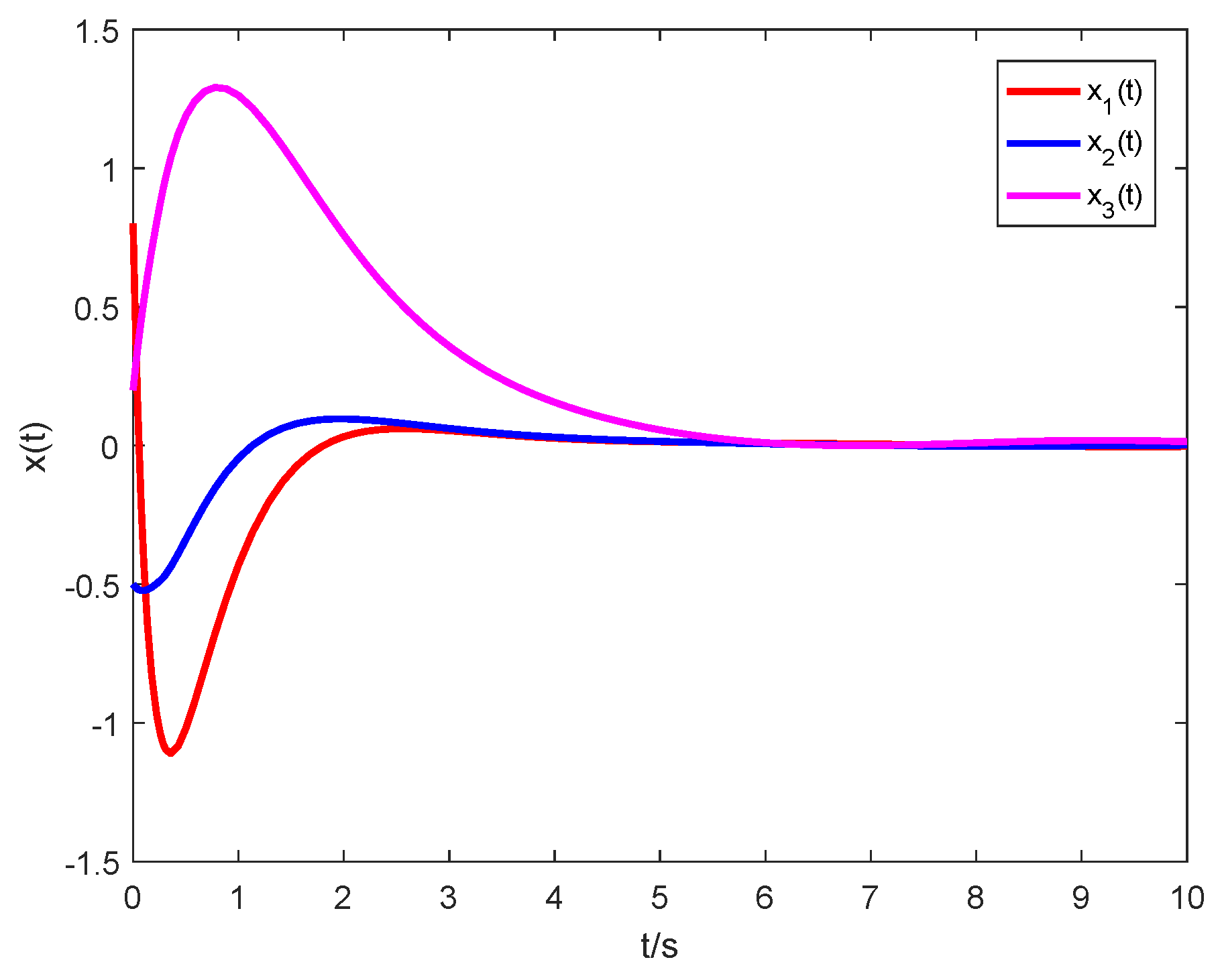
4. Numerical Example

In this section, a numerical example is given to illustrate the effectiveness of the proposed results.

This example deals with a truck-trailer system with time-varying delay. The dynamic model is described as follows:

$$\left\{\begin{array}{c}{\dot{x}}_1\left(t\right)=-a\frac{v\overline{t}}{L{t}_0}{x}_1\left(t\right)-(1-a)\frac{v\overline{t}}{L{t}_0}{x}_1(t-d\left(t\right))+\frac{v\overline{t}}{l{t}_0}u\left(t\right)+{\omega }_1\left(t\right)\hfill \\ {\dot{x}}_2\left(t\right)=a\frac{v\overline{t}}{L{t}_0}{x}_1\left(t\right)+(1-a)\frac{v\overline{t}}{L{t}_0}{x}_1(t-d\left(t\right))\hfill \\ {\dot{x}}_3\left(t\right)=\frac{v\overline{t}}{t_0}sin[x_2\left(t\right)+a\frac{v\overline{t}}{L}{x}_1\left(t\right)+(1-a)\frac{v\overline{t}}{2L}{x}_1(t-d\left(t\right))]\hfill \end{array}\right.$$

where $x_1\left(t\right)$ is the angle difference between the truck and the trailer, $x_2\left(t\right)$ is the angle of the trailer, $x_3\left(t\right)$ represents the vertical position of the rear end of the trailer, $u\left(t\right)$ denotes the steering angle, $\omega \left(t\right)={\left({\omega }_1^T\left(t\right)\hspace{1em}{\omega }_2^T\left(t\right)\hspace{1em}{\omega }_3^T\left(t\right)\right)}^T$ is the exogenous disturbance.

Let $\sigma \left(t\right)=x_2\left(t\right)+a\frac{v\overline{t}}{L}{x}_1\left(t\right)+(1-a)\frac{v\overline{t}}{2L}{x}_1(t-d\left(t\right))$, the T-S fuzzy time-delay system that represents the above truck-tailer model is as follows:

Plant Rule 1: If $\sigma \left(t\right)$ is about 0, then

$$\begin{array}{c}\hfill \dot{x}\left(t\right)=A_{1}x\left(t\right)+A_{d1}x(t-d\left(t\right))+B_{1}u\left(t\right)+B_{\omega 1}\omega \left(t\right);\end{array}$$

Plant Rule 2: If $\sigma \left(t\right)$ is about $\pm \pi$, then

$$\begin{array}{c}\hfill \dot{x}\left(t\right)=A_{2}x\left(t\right)+A_{d2}x(t-d\left(t\right))+B_{2}u\left(t\right)+B_{\omega 2}\omega \left(t\right),\end{array}$$

where

$$\begin{array}{c}\hfill A_1=\left(\begin{array}{ccc}-a\frac{v\overline{t}}{L{t}_0}& 0& 0\\ a\frac{v\overline{t}}{L{t}_0}& 0& 0\\ a\frac{v^2{\overline{t}}^2}{2L{t}_0}& \frac{v\overline{t}}{t_0}& 0\end{array}\right),\hspace{1em}{A}_{d1}=\left(\begin{array}{ccc}-b\frac{v\overline{t}}{L{t}_0}& 0& 0\\ b\frac{v\overline{t}}{L{t}_0}& 0& 0\\ b\frac{v^2{\overline{t}}^2}{2L{t}_0}& 0& 0\end{array}\right),\end{array}$$

$$\begin{array}{c}\hfill A_2=\left(\begin{array}{ccc}-a\frac{v\overline{t}}{L{t}_0}& 0& 0\\ a\frac{v\overline{t}}{L{t}_0}& 0& 0\\ a\frac{d{v}^2{\overline{t}}^2}{2L{t}_0}& \frac{dv\overline{t}}{t_0}& 0\end{array}\right),\hspace{1em}{A}_{d2}=\left(\begin{array}{ccc}-b\frac{v\overline{t}}{L{t}_0}& 0& 0\\ b\frac{v\overline{t}}{L{t}_0}& 0& 0\\ b\frac{d{v}^2{\overline{t}}^2}{2L{t}_0}& 0& 0\end{array}\right),\end{array}$$

$$\begin{array}{c}\hfill B_1=B_2=\left(\begin{array}{c}\frac{v\overline{t}}{l{t}_0}\\ 0\\ 0\end{array}\right),\hspace{1em}\hspace{1em}{B}_{\omega 1}=B_{\omega 2}=\left(\begin{array}{ccc}1& 0& 0\\ 0& 0& 0\\ 0& 0& 0\end{array}\right),\end{array}$$

with $a+b=1$.

In order to illustrate the developed results, we borrow the model parameters from [36], such as $a=0.7$, $v=-1.0$, $L=5.5$, $l=2.8$, $\overline{t}=2.0$, $t_0=0.5$, and $d=10t_0/\pi$. The membership functions are defined as ${\rho }_1\left(x\left(t\right)\right)=1/\left(1+exp(x_1\left(t\right)+0.5)\right)$, ${\rho }_2\left(x\left(t\right)\right)=1-{\rho }_1\left(x\left(t\right)\right)$. Additionally, the other parameters involved in the simulation are chosen as $c_1=1$, $\delta =0.3$, $\beta =0.01$, $\gamma =0.8$, $T_f=10$, $R=I$, ${\mu }_1=-0.1$, ${\mu }_2=0.1$, and $h=0.6$. We aim to design a memory state feedback controller such that the resulting closed-loop T-S fuzzy time-delay system is finite-time bounded. By solving the LMI-based finite-time stabilization criterion proposed in Theorem 2 using the Matlab LMI toolbox, we can derive the feasible solutions for the optimal minimum value of $c_2=2.8830$. Furthermore, all the control gain matrices are obtained as follows:

$$\begin{array}{c}\hfill K_{11}=L_{11}{X}^{-1}=\left(\begin{array}{ccc}6.9875& -13.5452& 1.4041\end{array}\right),\hspace{1em}{K}_{12}=L_{12}{X}^{-1}=\left(\begin{array}{ccc}6.9871& -13.7540& 1.3966\end{array}\right),\end{array}$$

$$\begin{array}{c}\hfill K_{21}=L_{21}{X}^{-1}=\left(\begin{array}{ccc}0.3679& 0.0085& -0.0010\end{array}\right),\hspace{1em}{K}_{22}=L_{22}{X}^{-1}=\left(\begin{array}{ccc}0.3861& -0.0013& 0.0001\end{array}\right).\end{array}$$

For the simulation framework, the exogenous disturbance is selected as $\omega \left(t\right)={(0.06sint\hspace{1em}0\hspace{1em}0)}^T$, and the time-varying delay is assumed to be $d\left(t\right)=0.25+0.25sin\left(0.3t\right)$. For the initial condition $x\left(0\right)={(0.8\hspace{1em}-0.5\hspace{1em}0.2)}^T$, the state response of the corresponding closed-loop T-S fuzzy time-delay system is depicted in Figure 1, and the evolution of $x^T\left(t\right)Rx\left(t\right)$ is shown in Figure 2. From the simulation results, it is obvious that the closed-loop T-S fuzzy time-delay system is finite-time bounded with respect to $(1,2.8830,10,I,0.3,0.6)$ via the above memory state feedback controller. In addition, for different h, the optimal minimum values of $c_2$ for ensuring the closed-loop T-S fuzzy system finite-time bounded are summarized in

Table 1. The optimum bound values of $c_2$ for different h.

h	0.6	0.8	1.0	1.2	1.4
$c_2$	2.8830	3.6111	4.5002	5.7103	6.7601

. This proves the effectiveness of our developed results in Theorem 2.

5. Conclusions

In this paper, the problem of finite-time boundedness and finite-time stabilization for a class of T-S fuzzy time-delay systems was discussed. First, based on a new augmented LKF and by applying an improved reciprocally convex combination technique, a novel delay-dependent finite-time boundedness sufficient condition has been derived for an open-loop T-S fuzzy time-delay system. Secondly, a memory state feedback controller has been developed to ensure the finite-time boundedness of the corresponding closed-loop T-S fuzzy time-delay system. Finally, the effectiveness and advantages of the presented methods were demonstrated by a numerical example. Our future research work will focus on the problem of robust finite-time control for uncertain T-S fuzzy systems with time-varying delay and exogenous disturbance.

References

1. Wang, H.Q.; Liu, P.X.; Li, S.; Wang, D. Adaptive neural output-feedback control for a class of nonlower triangular nonlinear systems with unmodeled dynamics. IEEE Trans. Neural Netw. Learn. Syst. 2018, 29, 3658–3668. [Google Scholar]
2. Zhao, X.D.; Wang, X.Y.; Zhang, S.; Zong, G.D. Adaptive neural backstepping control design for a class of nonsmooth nonlinear systems. IEEE Trans. Syst. Man Cybern. Syst. 2019, 49, 1820–1831. [Google Scholar] [CrossRef]
3. Roy, S.; Kar, I.N. Adaptive sliding mode control of a class of nonlinear systems with artificial delay. J. Frankl. Inst. 2017, 354, 8156–8179. [Google Scholar] [CrossRef]
4. Qiu, J.B.; Sun, K.K.; Wang, T.; Gao, H.J. Observer-based fuzzy adaptive event-triggered control for pure-feedback nonlinear systems with prescribed performance. IEEE Trans. Fuzzy Syst. 2019, 27, 2152–2162. [Google Scholar] [CrossRef]
5. Vrabel, R. Eigenvalue based approach for assessment of global robustness of nonlinear dynamical systems. Symmetry 2019, 11, 569. [Google Scholar] [CrossRef] [Green Version]
6. Li, X.; Zhu, Z.C.; Rui, G.C.; Cheng, D.; Shen, G.; Tang, Y. Force loading tracking control of an electro-hydraulic actuator based on a nonlinear adaptive fuzzy backstepping control scheme. Symmetry 2018, 10, 155. [Google Scholar] [CrossRef] [Green Version]
7. Takagi, T.; Sugeno, M. Fuzzy identification of systems and its applications to modeling and control. IEEE Trans. Syst. Man Cybern. 1985, 15, 116–132. [Google Scholar] [CrossRef]
8. Zheng, W.; Wang, H.B.; Wang, H.R.; Wen, S.H. Stability analysis and dynamic output feedback controller design of T-S fuzzy systems with time-varying delays and external disturbances. J. Comput. Appl. Math. 2019, 358, 111–135. [Google Scholar] [CrossRef]
9. Tan, J.Y.; Dian, S.Y.; Zhao, T.; Chen, L. Stability and stabilization of T-S fuzzy systems with time delay via Wirtinger-based double integral inequality. Neurocomputing 2018, 275, 1063–1071. [Google Scholar] [CrossRef]
10. Seuret, A.; Gouaisbaut, F. Wirtinger-based integral inequality: Application to time-delay systems. Automatica 2013, 49, 2860–2866. [Google Scholar] [CrossRef] [Green Version]
11. Zhao, T.; Huang, M.B.; Dian, S.Y. Stability and stabilization of T-S fuzzy systems with two additive time-varying delays. Inform. Sci. 2019, 494, 174–192. [Google Scholar] [CrossRef]
12. Benzaouia, A.; Hajjaji, A.E. Conditions of stabilization of positive continuous Takagi-Sugeno fuzzy systems with delay. Int. J. Fuzzy Syst. 2018, 20, 750–758. [Google Scholar] [CrossRef]
13. Lian, Z.; He, Y.; Zhang, C.K.; Wu, M. Further robust stability analysis for uncertain Takagi-Sugeno fuzzy systems with time-varying delay via relaxed integral inequality. Inform. Sci. 2017, 409–410, 139–150. [Google Scholar] [CrossRef]
14. Zhao, T.; Dian, S.Y. State feedback control for interval type-2 fuzzy systems with time-varying delay and unreliable communication links. IEEE Trans. Fuzzy Syst. 2018, 26, 951–966. [Google Scholar] [CrossRef]
15. Liu, C.; Mao, X.; Xu, X.Z.; Zhang, H.B. Stability analysis of discrete-time switched T-S fuzzy systems with all subsystems unstable. IEEE Access 2019, 7, 50412–50418. [Google Scholar] [CrossRef]
16. An, J.Y.; Lin, W.G. Improved stability criteria for time-varying delayed T-S fuzzy systems via delay partitioning approach. Fuzzy Sets Syst. 2011, 185, 83–94. [Google Scholar] [CrossRef]
17. Yang, J.; Luo, W.P.; Wang, Y.H.; Duan, C.S. Improved stability criteria for T-S fuzzy systems with time-varying delay by delay-partitioning approach. Int. J. Control Autom. Syst. 2015, 13, 1521–1529. [Google Scholar] [CrossRef]
18. Zeng, H.B.; Park, J.H.; Xia, J.W.; Xiao, S.P. Improved delay-dependent stability criteria for T-S fuzzy systems with time-varying delay. Appl. Math. Comput. 2014, 235, 492–501. [Google Scholar] [CrossRef]
19. Kwon, O.M.; Park, M.J.; Lee, S.M.; Park, J.H. Augmented Lyapunov–Krasovskii functional approaches to robust stability criteria for uncertain Takagi-Sugeno fuzzy systems with time-varying delay. Fuzzy Sets Syst. 2012, 201, 1–19. [Google Scholar] [CrossRef]
20. Wu, M.; He, Y.; She, J.H.; Liu, G.P. Delay-dependent criteria for robust stability of time-varying delay systems. Automatica 2004, 40, 1435–1439. [Google Scholar] [CrossRef]
21. Gu, K.; Kharitonov, V.L.; Chen, J. Stability of Time-Delay Systems; Birkhauser: Basel, Switzerland, 2003. [Google Scholar]
22. Park, P.G.; Ko, J.W.; Jeong, C. Reciprocally convex approach to stability of systems with time-varying delays. Automatica 2011, 47, 235–238. [Google Scholar] [CrossRef]
23. Park, P.; Lee, W.; Lee, S.Y. Auxiliary function-based integral inequalities for quadratic functions and their applications to time-delay systems. J. Frankl. Inst. 2015, 352, 1378–1396. [Google Scholar] [CrossRef]
24. Zeng, H.B.; He, Y.; Wu, M.; She, J.H. Free-matrix-based integral inequality for stability analysis of systems with time-varying delay. IEEE Trans. Autom. Control 2015, 60, 2768–2772. [Google Scholar] [CrossRef]
25. Liu, F.; Wu, M.; He, Y.; Yokoyamab, R. New delay-dependent stability criteria for T-S fuzzy systems with time-varying delay. Fuzzy Sets Syst. 2010, 161, 2033–2042. [Google Scholar] [CrossRef]
26. Lian, Z.; He, Y.; Zhang, C.K.; Wu, M. Stability analysis for T-S fuzzy systems with time-varying delay via free-matrix-based integral inequality. Int. J. Control Autom. Syst. 2016, 14, 21–28. [Google Scholar] [CrossRef]
27. Amato, F.; Ariola, M.; Dorato, P. Finite-time control of linear systems subject to parametric uncertainties and disturbances. Automatica 2001, 37, 1459–1463. [Google Scholar] [CrossRef]
28. Liu, H.; Shi, P.; Karimi, H.R.; Chadli, M. Finite-time stability and stabilisation for a class of nonlinear systems with time-varying delay. Int. J. Syst. Sci. 2016, 47, 1433–1444. [Google Scholar] [CrossRef]
29. Huang, X.P.; Wu, C.Y.; Liu, Y.P. Finite-time H model reference control of SLPV systems and its application to aero-engines. IEEE Access 2019, 7, 43525–43533. [Google Scholar] [CrossRef]
30. Ma, R.C.; Jiang, B.; Liu, Y. Finite-time stabilization with output-constraints of a class of high-order nonlinear systems. Int. J. Control Autom. Syst. 2018, 16, 945–952. [Google Scholar] [CrossRef]
31. Sakthivel, R.; Saravanakumar, T.; Kaviarasan, B.; Lim, Y.D. Finite-time dissipative based fault-tolerant control of Takagi-Sugeno fuzzy systems in a network environment. J. Frankl. Inst. 2017, 354, 3430–3455. [Google Scholar] [CrossRef]
32. Ren, C.C.; Ai, Q.L.; He, S.P. Finite-time non-fragile control of a class of uncertain linear positive systems. IEEE Access 2019, 7, 6319–6326. [Google Scholar] [CrossRef]
33. Zhang, X.M.; Han, Q.L.; Seuret, A.; Gouaisbaut, F. An improved reciprocally convex inequality and an augmented Lyapunov–Krasovskii functional for stability of linear systems with time-varying delay. Automatica 2017, 84, 221–226. [Google Scholar] [CrossRef] [Green Version]
34. Cao, Y.Y.; Frank, P.M. Stability analysis and synthesis of nonlinear time-delay systems via linear Takagi-Sugeno fuzzy models. Fuzzy Sets Syst. 2001, 124, 213–229. [Google Scholar] [CrossRef]
35. Han, L.; Qiu, C.Y.; Xiao, J. Finite-time H control synthesis for nonlinear switched systems using T-S fuzzy model. Neurocomputing 2016, 171, 156–170. [Google Scholar] [CrossRef]
36. Yan, H.C.; Wang, T.T.; Zhang, H.; Shi, H.B. Event-triggered H control for uncertain networked T-S fuzzy systems with time delay. Neurocomputing 2015, 157, 273–279. [Google Scholar] [CrossRef]
Figure 1. The state response of the closed-loop Takagi–Sugeno fuzzy system.
Symmetry 12 00447 g001
Figure 2. The time history of x T ( t ) R x ( t ) .
Symmetry 12 00447 g002