Article

A Low-Rank Tensor Factorization Using Implicit Similarity in Trust Relationships

School of Information Science and Engineering, Xinjiang University, Urumqi 830046, China
*
Author to whom correspondence should be addressed.
Symmetry 2020, 12(3), 439; https://doi.org/10.3390/sym12030439
Submission received: 5 January 2020 / Revised: 2 March 2020 / Accepted: 3 March 2020 / Published: 9 March 2020

Abstract

:
Low-rank tensor factorization can not only mine the implicit relationships between data but also fill in the missing data when working with complex data. Compared with the traditional collaborative filtering (CF) algorithm, the changes are essentially proposed, from traditional matrix analysis to three-dimensional spatial analysis. Based on low-rank tensor factorization, this paper proposes a recommendation model that comprehensively considers local information and global information, in other words, combining the similarity between trust users and low-rank tensor factorization. First, the similarity between trusted users is measured to capture local information between users by trusting similar preferences of users when selecting items. Then, the users’ similarity is integrated into the tensor, and the low-rank tensor factorization is used to better maintain and describe the internal structure of the data to obtain global information. Furthermore, based on the idea of the alternating least squares method, the conjugate gradient (CG) optimization algorithm for the model of this paper is designed. The local and global information is used to generate the optimal expected result in an iterative process. Finally, we conducted a large number of comparative experiments on the Ciao dataset and the FilmTrust dataset. Experimental results show that the algorithm has less precision loss under the data set with lower density. Thus, not only can a perfect compromise between accuracy and coverage be achieved, but also the computational complexity can be reduced to meet the need for real-time results.

1. Introduction

Currently, in a network environment in which data amounts are soaring, the traditional ‘resource retrieval’ method on the Internet has long been unable to meet the needs of users [1]. In the new era, the best method of Internet information dissemination is to automatically present information to users according to their choices. The recommendation system has come into being [2]. It can sort certain items based on certain strategic specifications, and display the items listed in the forefront to the user, which facilitates the user’s choice. The recommendation of information consultation not only provides convenience for the users, but also brings enormous benefits to the Internet industry. In addition, the recommendation algorithm has great research value as the core [3].
The collaborative filtering algorithm is the most widely used and successful algorithm in recommendation system [4]. It considers that users have similar preferences. The item recommendation is achieved by calculating a large amount of structured data to determine what items the user might like [5]. However, due to the large size of the data set, the structure is more complicated. User preferences are often influenced by other factors such as time, weather, geographic location, social relationships [6,7,8]. We call these factors context. These issues can greatly affect the accuracy of the CF algorithm [4,9]. Therefore, in the current research, a context-based recommendation system that extends from the traditional user-item two-dimensional factor to the user-item-context three-dimensional factor is gradually considered [10].
Tensor [11], a multidimensional array, is regarded as an important tool for representing unstructured and complex data, with the goal of pushing vectors and matrices to higher dimensions. Low-rank tensor factorization is essentially a high-order generalization of matrix factorization [10,12]. It has three major advantages when processing data, namely dimension reduction processing, missing data filling, and implicit relationship mining [13]. Low-rank tensor factorization is applied to the recommendation system, including multidimensional data of at least three dimensions as a consideration. Any combination of time, place, subject, user friend, and other related variables can be considered in the process of accommodating context information [14]. Correlation analysis of these sparse data is performed by low-rank tensor factorization to find the intrinsic relationships in the data. The validity and accuracy of the tensor algorithm in a multidimensional factor recommendation system are proved in these research processes [15]. However, some important issues have not been fully resolved, such as cold start, sparsity, and data updates. In the existing research, only the regularization term in the tensor factorization is considered to be the influencing factor of the user’s social relationship [16], and the accuracy is low. The context-based tensor recommendation algorithm utilizes only a physical description between the items, ignoring the similarity between the user and the user’s preference for the item [17]. Our purpose is to obtain the similarity of preferences among local users and also to observe each item globally. Based on this, the optimization of the algorithm is proposed. In this paper, we propose a low-rank tensor factorization recommendation algorithm based on the implicit similarity of a trust relationship.
In summary, the contributions of this paper are threefold:
1. We propose that each user’s trust strength is not the same as their friends. First, we measure the implicit similarity between trusted users and obtain the local information between trusted users. These data are introduced into the low-rank tensor factorization to construct a new tensor model. The proposed new model is solved by a local correlation and global minimization algorithm. The user similarity measure and factor matrix regularization in the model can effectively improve the a priori condition of the model. This approach can not only improve the credibility of the recommendation but also ease the user’s cold start problem.
2. Based on the idea of the alternating least squares solution, the conjugate gradient optimization algorithm for the model of this paper is designed. The required storage is small, and the stability is high in the iterative process. The experimental comparison shows that the results are better than the stochastic gradient descent method.
3. We jointly take the rating and social relationship into consideration to improve the recommender systems. In addition, we propose to utilize the social relationship in a contextual prefiltering manner based on tensor factorization. Our experimental results show that the presented algorithm—compared with the SVD, improved SVDpp, BaselineOnly, KNNBaseline, and NMF results in a tiny loss of accuracy with the lower density datasets. Thus, it not only obtains a perfect tradeoff between the accuracy and coverage, but also provides an approach that can reduce the complexity of the computation and meet the real-time need.
The remainder of this article is as follows. Section 2 reviews previous work related to the proposed methodology. In Section 3, the operation of the new tensor model is introduced. Section 4 is the experimental part of this paper. The experimental results and discussion are given by comparison with the traditional recommendation algorithm. Section 5 is a summary of this article.

2. Related Studies

2.1. User-Based Collaborative Filtering

The user-based collaborative filtering (UCF) algorithm [18] is a domain-based algorithm and is the most basic algorithm used in recommendation systems. This algorithm was proposed in 1992 and marks the birth of the recommendation system. It was applied to a mail filtering system. GroupLens applied it to news filtering in 1994. One of the main tasks in UCF is to recognize the involved users that are most likely to have the same aim as a user. Therefore, the academic community has conducted a number of studies to propose a similarity method for solving these users [9]. Among them, Golbeck and Hendler [19] consider the relationship between users and users when evaluating indicators. Linden and Smith [20] consider the similarities between items. Although these methods are relatively successful, every method has its shortcomings. For example, an adequate quantity of evaluation values is needed to calculate the similarity between every pair of users. Nevertheless, a few users in the system did not give any feedback on the item. This issue will also affect new items in a new system and there is not any historical information. This problem also goes by the names of ‘cold start’ and ‘data sparse’. The cold start problem means that a new user or a new item does not have enough historical information. Data sparsity occurs when only a few users have commented on an item. A common way to solve these problems is to think about additional sources of information, and Moradi and Ahmadian [21] propose to consider friendships in social networks. Guo and Yorke-Smith [22] proposed a novel Bayesian similarity measure based on the Dirichlet distribution, which considers both the direction and length of the rating vectors. Ar and Bostanci [23] propose to calculate similar values to provide weights to adjacent users, and the identified adjacent users are applied to the predicted evaluation values. Al-Shamri and Bharadwaj [24] use direct prediction of unknown evaluation values without the need to find and weight similar users. These methods are applicable only to evaluation ratings, and they cannot effectively solve the problem of data sparsity. Agarwal and Bharadwaj [25] use GA to predict unknown evaluation values based on evaluation values and trust, to improve the accuracy of the recommendation results. Bedi and Sharma [26] proposed a method called the trust-based ant recommendation system (TAS), which metaphorizes the trust relationship between the users to the biology of ant colonies. TAS proposes a new method for calculating the trust value between users and unites it with the similarity value to generate a trust graph between users; then, it uses the ant colony algorithm to constantly renew the trust value between the user and the neighbor. These studies have fully considered that the similarity between users has an important impact on the recommendation results, but it does not account for the relevance of other factors, such as the time and location.

2.2. Low-Rank Tensor Factorization

In the process of in-depth research, the recommendation system proposes a new form that can represent complex data and heterogeneous information networks, namely, tensors. The low-rank tensor factorization applied to the recommendation system can usually consider the correlation between multidimensional factors, such as users, items, topics, contexts, and so on [27].
Symeonidis et al. [28] proposed introducing a label as a context factor in the low-rank tensor factorization recommendation algorithm, constructing a user-item-label three-dimensional tensor, and using a high-order singular value factorization method for tensor factorization. However, this method has been trained for a long time and is difficult to apply to actual recommendations. On the basis of Symeonidis, Rendle et al. [29] improved the process of tensor factorization and improved the operation speed while ensuring the accuracy of the algorithm. Later, Rendle improved the complexity of the algorithm and proposed a pairwise tensor factorization algorithm to further improve the recommendation quality [30]. Rafailidis and Daras [31] proposed a tensor factorization based on the label clustering method to mitigate data sparseness by clustering labels. Symeonidis et al. [32] also proposed a geographic recommendation system on account of a friend contact algorithm and high-order singular value factorization algorithm, which is suitable for user friend-location-activity. However, this method still cannot be linked to time information. To apply the spatiotemporal information to the point of interest recommendation, Ying et al. [33] used the context based on the user’s preference for tensor factorization. They also proposed a POI user preference inference model based on weighted Hyperlink-Induced Topic Search (HITS). In their research, the user’s social background was not accounted for. Ifada and Nayak [34] proposed a scalable tensor recommendation based on probability ordering and block parallel matrix multiplication. When new users and new items are added to the system, the system can generate an approximate tensor. Zheng et al. [35] proposed an individual recommendation model based on tensor factorization, which was provided as an item. This model measures the potential association between users and groups by considering social markers, partially alleviating the cold start problem. The recommendation algorithm based on tensor factorization is usually to build the context outside the user and item into the model. The algorithm is applied in different application scenarios by adding different context information. Karatzoglou et al. [36] proposed multiclass context information, using a high-order singular value factorization algorithm to construct a user-item-context tensor factorization model for personalized recommendation. These studies fully consider the influence of multidimensional factors on the recommendation results, and they explore the intrinsic relationship between contextual factors, but ignore the implicit similarity between users. Therefore, we are committed to effectively integrating user social information with contextual information for research.

2.3. Algorithm Optimization

Algorithm optimization is generally optimized for algorithm structure and convergence. It studies how to find the number of certain factors under given constraints to optimize some or some of the indicators. In machine learning, the essence of most algorithms is to build an optimization model and to optimize the objective function through optimization methods to train the best model. Our common optimization methods are the gradient descent (GD) method [37], stochastic gradient descent (SGD) method [38], Newton method [39], CG method [40], and so on.
The gradient descent method was proposed by the famous mathematician Cauchy in 1847 and is one of the simplest and oldest methods for solving unconstrained optimization problems. The gradient descent method is the most widely used and widely used algorithm in the field of machine learning. Its basic idea is that the next point to be searched in the direction of the negative gradient must be better than the original point, and there will be no meaningless iterations; thus, it is also a very classic algorithm for finding the minimum value. When the algorithm is close to the minimum value, the convergence speed is slowed down, and some problems can occur in the line search. Therefore, the early research content was mainly to update the parameters by processing small batches of data during each iteration, and approximated the true gradient on the entire data set by using gradients calculated from part of the data, thereby improving the shortcomings of the gradient descent algorithm, namely the stochastic gradient descent algorithm, which had large calculation density, and large storage space. This algorithm takes the loss of a small part of the precision and increases the number of iterations in exchange for the overall optimization efficiency. The proposed Newton method is applied to the optimization problem, which is an approximate method for solving equations in real and complex domains. It is a second-order convergence, which is faster than the first-order convergence of the gradient descent method. However, each step of the Newton method must solve the inverse matrix of the Hessian matrix of the objective function, and the calculation is complicated. Therefore, we choose the CG method between the SGD method and Newton method in the algorithm optimization problem.
The CG method was first introduced by Schmidt in 1908 [40], and its initial purpose was to solve linear symmetric positive definite equations. Hestenes and Stiefel [41] combined the convergent gradient method and statistical inversion methods in 1952 to propose an inversion algorithm that did not depend on the initial guess. Fletcher and Reeves [42] used the CG method of linear equations to solve unconstrained optimization problems in 1964. According to the definition of the step size and search direction of the CG method, the classical CG method is mainly divided into the Hestenes-Stiefel CG method [43], the Fletcher-Reeves CG method [42], the Polak-Ribiere-Polyak CG method [44], and the Dai-Yuan CG method [45]. When the objective function is a strictly convex quadratic function, the CG can show a good iterative effect. When the objective function is a general non-convex function, although some classic CG methods will have relatively good convergence, the numerical results will be different, and some will be difficult to meet the required accuracy. Meaning to construct a CG suitable for this type of objective function. Hager and Zhang [46] proposed a new CG method based on the self-tuning ratio BFGS method, which is globally convergent for strong convex functions. Dai and Kou [47] proposed the CGOPT method, which has global convergence under a modified Wolfe line search and has excellent numerical performance.
The CG method requires only the first derivative information of the objective function, but it overcomes the shortcomings of the slow convergence of the stochastic gradient method and avoids it. The Newton method requires the disadvantage of storing and computing the Hessian matrix and inverting it.

3. Method

3.1. Model Architecture

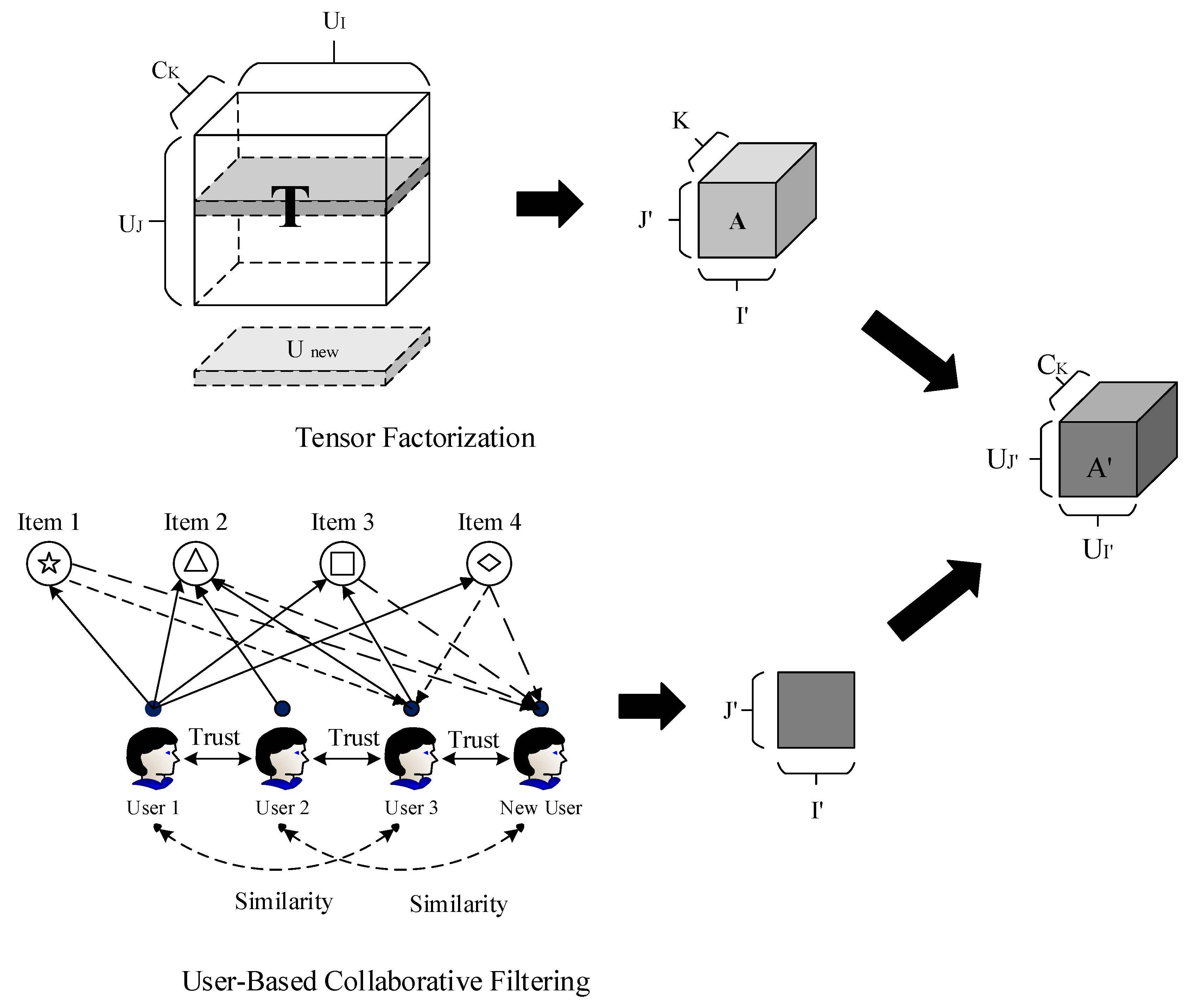
The architecture used in this paper is shown in Figure 1. The symbol descriptions in Figure 1 are shown in Table 1. This architecture includes two steps: (1) Solving the implicit similarity between trusted users based on user collaborative filtering, and (2) Predicting user ratings based on low-rank tensor factorization. On the basis of the existing tensor factorization, the approximate tensor A is calculated by an overall tensor T. In the calculation process—due to problems such as cold start, data sparseness, and large number of items—the calculation complexity is high and the use time is too long. The model proposed in this paper considers the implicit similarity between trusted users based on user collaborative filtering to provide local information between users. The user’s social network relationship is utilized to reduce the size of the computed low-rank tensor model. Therefore, the proposed size based on the implicit similarity tensor model A’ is significantly smaller than the typical tensor model T by two steps based on user collaborative filtering and basic low-rank tensor factorization. Figure 1 also includes the ability to generate and decompose the implicit similarity tensor model A’ in real time based on the user collaborative filtering model and the tensor factorization model during data update.

3.2. User-Based Collaborative Filtering

The joint study of sociology and computer science shows that the user’s behavior is influenced by its direct trust of friends. As the saying goes, “Birds of a feather flock together.” Take the movie as an example. If user A likes “Forrest Gump”, “When Happiness Comes Knocking”, “Rain Man”, “Shawshank Redemption”, and other movies, another user B also likes these movies. If he also likes “Wind and Harvard Road”, it is very likely that user A also likes the movie “Wind and Harvard Road”. Therefore, in the recommendation system, when user A needs a personalized recommendation, he can first find a user group M with similar interests. Then, it recommends to A an item that M likes and A has not touched, which is based on the UCF algorithm. As shown in Figure 1, the focus of this paper is to solve the similarity between trusted users by considering the implicit similarity between the trust relationship between users and user behavior.
Given user U and user V, assume that N(u) represents positive feedback information that user U has ever made on the item set, and N(v) represents positive feedback information that user V has ever made on the item set. Then, we can simply calculate the implicit similarity of interest between user U and user V, as in (1).
w u v =   i N ( u )   N ( v ) 1 log ( 1 + | N ( i ) | ) | N ( u ) | | N ( v ) |
In Equation (1), the 1 log ( 1 + | N ( i ) | ) effect of popular items in the common interest list of user U and user V on their implicit similarity is penalized.
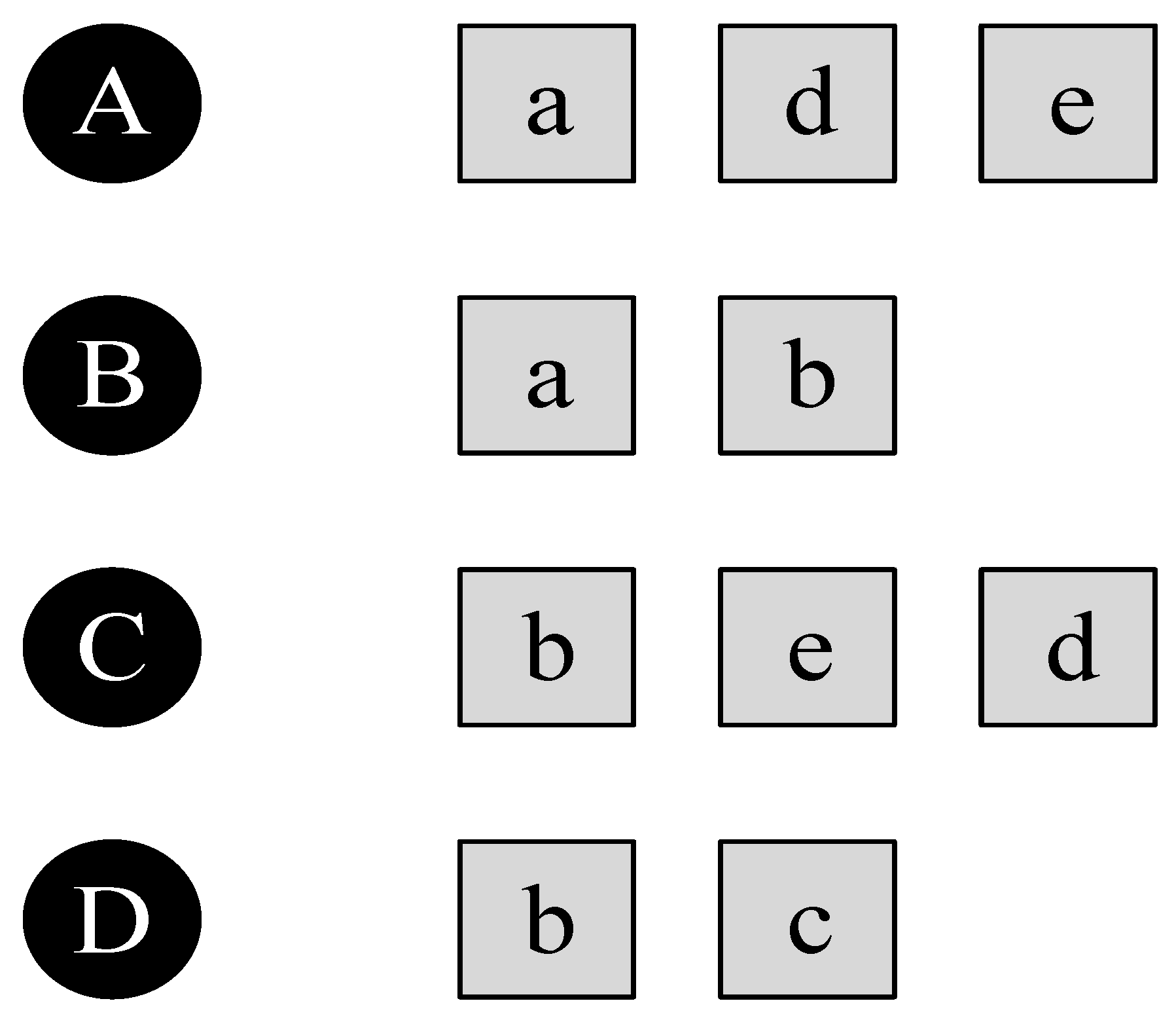
An example analysis is performed, as shown in Figure 2. It is assumed that user A has evaluated information for item {a, d, e}, and user B has evaluated information for item {a, b}. The implicit similarity between user A and user B is calculated using (1).
w A B =   i N ( A )   N ( B ) 1 log ( 1 + | N ( i ) | ) | N ( A ) | | N ( B ) | 1.356
By analogy, the implicit similarity between user A and users C and D can be obtained, and as shown in Table 2, the implicit similarity between user U and user V can be easily calculated by UCF.

3.3. Tensor Tucker Factorization Model

The tensor is the generalized concept of multidimensional arrays. Compared to matrix formats, tensors usually contain more basic structural information. Applying a tensor to a recommendation system can accurately capture the inherent correlations between users through multidimensional data to achieve more effective recommendation results. Although these data can be analyzed by matrix methods after expansion or flattening, such matrixing usually does not take full advantage of the essential tensor structure.
It appears to be natural to directly extend low-rank matrix factorization methods to the low-rank tensor factorization problem. Based on this definition, Ji et al. [48] further proposed a nonconvex approach. However, these methods involved the singular value decomposition (SVD) of Y ( n ) , which is time-consuming. To address this issue, Xu et al. [49] adopted low-rank matrix factorization:
m i n y , X n = 1 N α n 2 Y ( n ) X n F
where   Y ( n ) is the observed data, and X n is the projection operator.
In this paper, a third-order tensor is used as an example. As shown in Figure 3, suppose that T is the tensor of size I × J × K , which can be expressed as Tucker factorization:
T A × U I × V J × C K
where, the volume of the core tensor A is m × n × l , the user factor matrix is U A I × m , the item factor matrix is V A J × n , and the context factor matrix is C A K × l . Therefore, the score that corresponds to any position on the tensor T is:
T i j k m = 1 I n = 1 J l = 1 K ( A m n l × u i m × v j n × c k l )
The minimum loss function for the score tensor T factorization is:
minJ = 1 2 ( i , j , k ) T e i j k 2 = 1 2 ( i , j , k ) T ( T i j k m = 1 I n = 1 J l = 1 K ( A m n l × u i m × v j n × c k l ) ) 2
We solve u i m , v j n , c k l , and A m n l according to the SGD method. The update formula for each iteration is:
u i m u i m + α j , k : ( i , j , k ) T e i j k × ( n = 1 J l = 1 K ( A m n l × v j n × c k l ) )
v j n v j n + α i , k : ( i , j , k ) T e i j k × ( m = 1 I l = 1 K ( A m n l × u i m × c k l ) )
c k l c k l + α i , j : ( i , j , k ) T e i j k × ( m = 1 I n = 1 J ( A m n l × u i m × v j n ) )
A m n l A m n l + α ( i , j , k ) T e i j k × u i m × v j n × c k l
where α is the learning rate, and the summation subscripts j , k : ( i , j , k ) T , i , k : ( i , j , k ) T , and i , j : ( i , j , k ) T in the update formula represent the set of position indices of all nonzero elements on the matrix T ( i , : , : ) ,   T ( : , j , : ) ,   and   T ( : , : , k ) respectively. This method minimizes the factorization of kernel norms and low-rank tensors to effectively improve the inferiority of potential results.

3.4. A Low-Rank Tensor Factorization Using Implicit Similarity in Trust Relationships (LTF-ISTR)

In a real network, users do not exist independently, and there is a certain social relationship between users. The two users have different preferences for an item based on mutual trust. Therefore, based on the consideration of trusting users, this paper further considers the implicit similarity of users and captures the local information of correlation between users. After obtaining the association relationship of the trusted users, the global information between the users is further explored by low-rank tensor factorization.
This paper proposes a new tensor model, which is a low-rank tensor factorization using implicit similarity in trust relationships. Here, we define a third-order tensor T, where the tensor T i j k represents the score given by the user U i in the context of similarity C k and the same movie viewed by the trusted user U j , as shown in Figure 1. The matrix U I × U J of the user and the trusted user is obtained by user collaborative filtering, and the implicit similarity C k between the user U I and the trusted user U J is obtained. The approximate tensor A is reconstructed to generate a new low-rank tensor A based on the implicit similarity of the trust relationship. Then, Tucker factorization is performed on tensor A . The size of the core tensor A is m × n × l , the user U I factor matrix is U I A I × m , and the user U J factor matrix is U J A J × n , hidden. The matrix that contains the similarity factor is C k A K × l . Therefore, the objective function of the low-rank tensor factorization using implicit similarity in trust relationships is defined as:
L ( A , U I , U J , C K ) = 1 2 ( i , j , k ) A I ( i , j , k ) × ( A i j k m = 1 I n = 1 J l = 1 K ( A m n l × u i m × u j n × c k l ) ) 2 + 1 2 S i m ( u i , u j ) λ A | | A | | F 2 + λ 2 ( | | U I | | F 2 + | | U J | | F 2 + | | C K | | F 2 )
here, I ( i , j , k ) and S i m ( u i , u j ) are   defined   as :
I ( i , j , k ) = {   1 ,   if   A ( i , j , k )   0 ,   o t h e r w i s e
S i m ( u i , u j ) = {   1 ,   if   ( u i   u j )   0 ,   o t h e r w i s e
Among them, S i m ( u i , u j ) λ A is a positive regularization parameter, and | | U I | | F 2 ,   | | U J | | F 2 ,   | | C K | | F 2 denotes the L2 norm regularization term of each factor matrix. Our model considers a priori the trust user factor matrix and has a deeper insight into the factor matrix prior. There is further optimization of the low-rank tensor factorization.
Next, we chose the CG method between the SGD method and Newton method in the algorithm optimization problem. The CG method can quickly converge to the optimal solution of the solved problem when solving large linear equations, and it has the advantage of small storage. Its basic idea is to construct a set of conjugate directions in the direction of the negative gradient at the iteration point and then to search the target function extremum along this set of directions. The CG method has a good local search ability, and the solution process is as follows:
  • Step 1: Select the initial point X 0 , given the precision e p s , and let k = 0 ;
  • Step 2: Calculate g 0 = f ( X 0 ) , if g 0 = 0 , stop; otherwise, d 0 = g 0 ;
  • Step 3: Calculate λ k = g k T d k d k T A d k ;
  • Step 4: Calculate X k + 1 = X k + λ k d k ;
  • Step 5: Calculate g k + 1 = f ( X k + 1 ) , if g k + 1 = 0 , stop;
  • Step 6: Calculate d k + 1 = g k + 1 + g k + 1 T A d k + 1 d k T A d k d k ;
  • Step 7: Let k = k + 1 and go to Step 3.
According to the above steps, for the positive definite quadratic function. First, we initialize the values, and then iteratively update them by Formula (12). The iterative formula of the CG method is:
{ X k + 1 = X k + λ k d k g k + 1 = f ( X k + 1 ) d k + 1 = g k + 1 + β k d k
here,
β k = g k + 1 T A d k + 1 d k T A d k
λ k = g k T d k d k T A d k
In these processes, we know that the calculation formula for the coefficient β k in the search direction d k + 1   =   g k + 1   +   β k d k contains a symmetric and positive definite matrix A. It can be seen that to extend the CG method of application and quadratic function to general functions, we must first solve that the matrix A cannot be included in the formula.
The solution is:
(1) Use the Fletcher–Reeves CG method [42] when calculating, that is:
β k = g k + 1 T g k + 1 g k T g k
(2)   λ k is obtained by using Wolfe’s linear search criterion, which has quadratic termination [45].
In our model, the Fletcher-Reeves CG method requires a small amount of storage, is stable and does not require any external parameters, and it greatly improves the computational efficiency. The objective function L ( A , U I , U J , C K ) is optimized by the Fletcher–Reeves CG method. The local minimum parameters u i m , u j n , c k l and A m n l are obtained according to the following formula.
Taking u i m as an example, the calculation steps are as follows:
  • Step 1: Select the initial point u i m , given error accuracy > 0 , let k = 1 ;
  • Step 2: Calculate L u i m   =   f ( u i m ) , if L u i m   <   E , stop. Otherwise, take the next step;
  • Step 3: Construct search direction, let d i m   =   L u i m   +   β d i m and β   =   ( L u ( i + 1 ) ( m + 1 ) ) T L u ( i + 1 ) ( m + 1 ) ( L u i m ) T L u i m ;
  • Step 4: let u ( i + 1 ) ( m + 1 )   =   u i m   +   λ k d i m and the Wolfe linear search criterion is used to calculate the step size λ k . A new iteration point is obtained. Return to Step 2.
    u i m { u i m + λ k d i m d i m = L u i m + β d i m β = ( L u ( i + 1 ) ( m + 1 ) ) T L u ( i + 1 ) ( m + 1 ) ( L u i m ) T L u i m
    by the same token,
    u j n { u j n + λ k d j n d j n = L u j n + β d j n β = ( L u ( j + 1 ) ( n + 1 ) ) T L u ( j + 1 ) ( n + 1 ) ( L u j n ) T L u j n
    c k l { c k l + λ k d k l d k l = L c k l + β d k l β = ( L c ( k + 1 ) ( l + 1 ) ) T L c ( k + 1 ) ( l + 1 ) ( L c k l ) T L c k l
    A m n l { A m n l + λ k d m n l d m n l = L A m n l + β d m n l β = ( L A ( m + 1 ) ( n + 1 ) ( l + 1 ) ) T L A ( m + 1 ) ( n + 1 ) ( l + 1 ) ( L A m n l ) T L A m n l
It should be noted that in the low-rank tensor model of this paper, the user U I and the user U J have the same number. Trusting users is part of the overall user. Therefore, a low-rank tensor factorization using implicit similarity in trust relationship is significantly smaller than the traditional tensor model. In addition, there is no need to calculate the overall tensor T when the user updates.
In our model, the low-rank factorization fidelity term is used to capture global information, while the implicit similarity of the trusted user and the regularization term of each factor matrix are used to capture local information. Therefore, our approach utilizes local and global information and is reasonably expected to produce better results.
4. Experiments

4.1. Dataset

This paper makes use of public dataset Ciao and FilmTrust with user trust relationships for experimental verification [5,50].
The Ciao dataset was collected and published by Tang et al. in 2011, which included social networks and rating information. After registering a website, users can comment and rate all items. They can also browse other users’ reviews and ratings of products to help users make prejudgments when selecting products. Users on the website can also establish friendships through trust. The user’s rating on the website ranges from 1 to 5 (low to high). If there is a trust relationship between users, the measure is 1. A detailed description of the Ciao dataset is shown in Table 3.
The FilmTrust dataset is a small dataset that was captured from the entire FilmTrust website in June 2011. It contains the user’s rating data for the movie and the trust relationship data between users. The user’s rating on the website ranges from 0.5 to 4 (low to high preference). If there is a trust relationship between users, the measure is 1. A detailed description of the FilmTrust data set is shown in Table 3.

4.2. Evaluation Index

When evaluating algorithm performance, we evaluate the pros and cons of the algorithm based on the accuracy of the recommended predictions. For classification models, the main indicators for evaluating the accuracy of recommendations are: precision, recall, coverage, and novelty [28]. For scoring prediction models, the main indicators of accuracy that can be evaluated are: root mean square error (RMSE) and mean absolute error (MAE) [51].
The intent of this paper model is to predict the user’s rating of an item. Therefore, to evaluate the performance of the algorithm, we use the MAE and the RMSE as the evaluation indicators. Both MAE and RMSE apply to the predicted scenario, both of which reflect the accuracy of the predicted score. The smaller the values of MAE and RMSE are, the better the performance of the algorithm, considering only the accuracy.
The metric MAE is defined as:
MAE = 1 N ( i , j , k ) T | T ijk A ijk |
The metric RMSE is defined as:
RMSE = ( i , j , k ) T ( T ijk A ijk ) 2 N
where N is the number of predicted ratings, T is the data for all test sets, T ijk is the number of true ratings, and A ijk is the number of predicted ratings.

4.3. Experimental Results and Analysis

4.3.1. Experiment 1: Parameter Value

In the Fletcher-Reeves CG method, the learning rate is the speed at which the parameter reaches the optimal value. When the learning rate is too large, in other words, the rate of decline is fast, it is likely to cross the optimal value at some step. When the learning rate is too small, the decline is slow and cannot converge for a long time. Therefore, the learning rate directly determines the performance of the learning algorithm. The regularization term is to avoid overfitting problems during the learning process. In the course of the experiment, it is necessary to select the value of the learning rate α, the coefficient λ of the regularization term, and the number of iterations. Among them, we assume λ_A’ = λ. Through a large number of experiments, it is best to obtain a regularization term of 0.01 [51].
The choice the of learning rate changes. We first assume that the coefficient of the regularization term is 0.01, and then, we set the iteration update number to n = 20. In the trust relationship proposed in this paper, we use collaborative filtering methods to calculate similarity preferences among users, and then use implicit similarity to perform experiments on low-order tensor factorization. In the course of the experiment, the choice of the value of the learning rate is very important. For this, we choose to do the experiment among 0.0001–0.1.
It can be seen from Table 4 and Table 5 that when the learning rate is gradually increasing, the falling speed is too fast, and the optimal value cannot be obtained; in addition, the values of the MAE and RMSE cannot be calculated. When the learning rate is 0.0001, the learning speed is too slow, which causes the values of MAE and RMSE to be too large, thus affecting the performance of the algorithm. Therefore, through experiments, we have the best learning outcome when we choose a learning rate of 0.001.
In the CG method, the number of iteration updates also affects the final local minimum parameter value. We chose the Fletcher-Reeves CG method in the experimental part. It can get rid of the influence of the symmetric positive definite matrix in the experimental calculation process, and it does not affect the final experimental results. First, the learning rate is set to 0.001, and the coefficient of the regularization term is 0.01. Experiments were conducted in a low-rank tensor model based on the implicit similarity of trusted users by selecting different iteration update times. The experimental results are shown in Table 6 and Table 7. As the number of iterations increases, the values of MAE and RMSE gradually converge. After the number of iterations reached 60, it gradually became stable. Due to the increase in the number of iterations, the algorithm time increases linearly. The number of iterations is doubled, and the time taken by the algorithm is approximately doubled. Considering both the duration of the algorithm and the experimental results, we decided to use the experimental results with iterations of 60 as the optimal result.

4.3.2. Experiment 2: Comparison between the Fletcher-Reeves CG Method and SGD Method

We chose the Fletcher-Reeves CG method and the SGD method for comparison. As shown in Table 8 and Table 9, we performed experimental comparisons in a low-rank tensor model based on the implicit similarity of trusted users. Here, we choose the same learning rate α   =   0.001 , the coefficient of the regularization term λ   =   0.01 , and the number of iterations n   =   60 . The results show that for a given number of iterations, when the SGD method is close to the optimal value, the efficiency is reduced. The Fletcher-Reeves CG method not only overcomes the shortcomings of the slow convergence speed of the SGD method, but also supports the limitation of a symmetric positive definite matrix and has high stability.

4.3.3. Experiment 3: Algorithm Comparison

A low-rank tensor factorization using implicit similarity in trust relationships is compared with other recommended algorithms to test the recommended effect of the algorithm. The comparison methods include TF, SVDpp, SVD, BaselineOnly, KNNBaseline, and NMF, as shown in Table 10. The experimental outcomes are shown in Table 11, in which the numerical results of MAE and RMSE of LTF-ISTR are the best, and the performance of the algorithm is better than that of the other comparison algorithms. In addition, the traditional TF algorithm is second. By comparing the running time of the algorithm, the TF algorithm has the longest duration, the LTF-ISTR algorithm is second, and the SVD, BaselineOnly, KNNBaseline, and NMF algorithms have shorter durations, all within 7 s. The comprehensive experimental results and algorithm duration can be seen; although the TF and LTF-ISTR algorithms have good experimental results, the algorithm has high complexity and it takes a long time. The LTF-ISTR algorithm proposed in this paper improves the computational complexity, and the calculation duration is smaller than the basic TF algorithm. The prediction performance of the recommendation system is superior to that of other algorithms.
Since the FilmTrust dataset contains only users, items and users’ ratings information, the basic TF algorithm cannot be implemented. The basic TF algorithm requires at least three influencing factors in addition to users’ ratings, such as the time, location and topic. On the FilmTrust dataset, we respectively compared the proposed algorithm, SVDpp, SVD, BaselineOnly, KNNBaseline, and NMF algorithms. As shown in Table 12, the numerical results of MAE and RMSE on LTF-ISTR are the best, and the performance of the algorithm is better than that of the other comparison algorithms. The LTF-ISTR algorithm runs much longer than the other algorithms, which is also a drawback of the proposed algorithm. Therefore, it is necessary to further explore the influencing factors of the algorithm operation in the algorithm duration.

4.3.4. Experiment 4: Comparison of the Sparseness of Different Ratings

To test the robustness of the proposed algorithm to different data densities, we set up experimental comparisons under different densities on the Ciao and FilmTrust datasets. The density of the dataset is 3%, 2%, and 1%, respectively. Other parameters are fixed. Table 13 and Table 14 show the results of the experiments performed by the LTF-ISTR algorithm and other algorithms under the different density datasets.
Through experimental comparison, as shown in Table 13 and Table 14, the LTF-ISTR algorithm is superior to other algorithms in MAE and RMSE under different data densities. This is because in solving the problem of data sparsity, the LTF-ISTR model has stronger linear data analysis ability, and can better analyze the data from a global perspective through the correlation among various items. This finding shows that in low-density data sets, the LTF-ISTR algorithm also has the ability of mining implicit relationships in user social data. In addition, with the decrease in the data set density, the algorithm also has good performance and good robustness. In summary, the LTF-ISTR algorithm is suitable for rating data sets of different densities.

5. Conclusions

This paper first analyzes the user’s social network relationships and context information, and it proposes a low-rank tensor model recommendation method based on the implicit similarity of trust users for sparse and cold-start problems. In our model, the low-rank factorization fidelity term is used to capture global information, while the implicit similarity of the trusted user and the regularization term of each factor matrix are used to capture local information. Therefore, our method utilizes local and global information to effectively improve the prior conditions of the model, which can not only improve the reliability of the recommendation, but also alleviate the user’s cold start problem. For the problem of data sparseness, our method analyzes it from a global perspective, better captures the linear relationship among the data, and can reasonably expect to produce better results. Data set experiments show that the proposed model has higher precision than other algorithms and is far superior to the traditional low-rank tensor factorization algorithm in its calculation time. Experiments also show that the algorithm has good effects under different sparse data sets and that it is also suitable for data sets with less sparsity.

Author Contributions

Conceptualization, J.Q.; Data curation, P.M. and L.W.; Formal analysis, J.Q.; Funding acquisition, L.W. and J.Q.; Methodology, J.Q.; Resources, P.M. and L.W.; Supervision, J.Q.; Validation, P.M. and L.W.; Writing—original draft, P.M.; Writing—review and editing, P.M., L.W., and J.Q. All authors have read and agreed to the published version of the manuscript.

Funding

The research was supported in part by the National Science Foundation of China under Grant No. 61867006 and No. 61771416. The Doctoral Scientific Research Foundation of Xinjiang University under Grant No. BS150263. The Education Reform Project of Higher Education of Xinjiang Uygur Autonomous Region Named A study on the application of teaching method combining MOOCs with flipping classroom. The Higher Education Innovation Project of Xinjiang Uygur Autonomous Region under Grant No. XJEDU2017T002. The authors would like to thank the anonymous reviewers for their constructive comments that helped to improve the quality of this paper.

Conflicts of Interest

The authors declare no conflict of interest.

References

  1. Bobadilla, J.; Ortega, F.; Hernando, A.; Gutiérrez, A. Recommender systems survey. Knowl. Based Syst. 2013, 46, 109–132. [Google Scholar] [CrossRef]
  2. Hernández-Rubio, M.; Cantador, I.; Bellogín, A. A comparative analysis of recommender systems based on item aspect opinions extracted from user reviews. User Modeling User Adapt. Interact. 2019, 29, 381–441. [Google Scholar] [CrossRef]
  3. Choi, K.; Suh, Y. A new similarity function for selecting neighbors for each target item in collaborative filtering. Knowl. Based Syst. 2013, 37, 146–153. [Google Scholar] [CrossRef]
  4. Jeong, H.; Chak, J. An Efficient MapReduce-Based Parallel Processing Framework for User-Based Collaborative Filtering. Symmetry 2019, 11, 748. [Google Scholar] [CrossRef] [Green Version]
  5. Yadav, S.; Kumar, V.; Sinha, S.; Nagpal, S. Trust aware recommender system using swarm intelligence. J. Comput. Sci. 2018, 28, 180–192. [Google Scholar] [CrossRef]
  6. Ma, H.; King, I.; Lyu, M.R. Mining web graphs for recommendations. IEEE Trans. Knowl. Data Eng. 2011, 24, 1051–1064. [Google Scholar] [CrossRef]
  7. Zheng, V.W.; Zheng, Y.; Xie, X.; Yang, Q. Towards mobile intelligence: Learning from GPS history data for collaborative recommendation. Artif. Intell. 2012, 184, 17–37. [Google Scholar] [CrossRef] [Green Version]
  8. Prims, O.T.; Castrillo, M.; Acosta, M.C.; Oriol, M.V.; Lorente, A.S.; Serradell, K.; Cortés, A.; Francisco, J.D.R. Finding, analysing and solving MPI communication bottlenecks in Earth System models. J. Comput. Sci. 2019, 36, 100864. [Google Scholar] [CrossRef]
  9. Kim, K.S.; Chang, D.S.; Choi, Y.S. Boosting Memory-Based Collaborative Filtering Using Content-Metadata. Symmetry 2019, 11, 561. [Google Scholar] [CrossRef] [Green Version]
  10. Maroulis, S.; Boutsis, I.; Kalogeraki, V. Context-aware point of interest recommendation using tensor factorization. In Proceedings of the 2016 IEEE International Conference on Big Data (Big Data), Washington, DC, USA, 5–8 December 2016; pp. 963–968. [Google Scholar]
  11. Jiang, T.X.; Huang, T.Z.; Zhao, X.L.; Ji, T.Y.; Deng, L.J. Matrix factorization for low-rank tensor completion using framelet prior. Inf. Sci. 2018, 436, 403–417. [Google Scholar] [CrossRef]
  12. Zhao, J.; Sun, G. Detect User’s Rating Characteristics by Separate Scores for Matrix Factorization Technique. Symmetry 2018, 10, 616. [Google Scholar] [CrossRef] [Green Version]
  13. Hong, M.; Jung, J.J. Mymoviehistory: Social recommender system by discovering social affinities among users. Cybern. Syst. 2016, 47, 88–110. [Google Scholar] [CrossRef]
  14. Zou, B.; Li, C.; Tan, L.; Chen, H. Gputensor: Efficient tensor factorization for context-aware recommendations. Inf. Sci. 2015, 299, 159–177. [Google Scholar] [CrossRef]
  15. Li, X.; Jiang, M.; Hong, H.; Liao, L.J. A time-aware personalized point-of-interest recommendation via high-order tensor factorization. ACM Trans. Inf. Syst. 2017, 35, 31. [Google Scholar] [CrossRef]
  16. Ma, H.; Yang, H.; Lyu, M.R.; King, I. Sorec: Social recommendation using probabilistic matrix factorization. In Proceedings of the 17th ACM Conference on Information and Knowledge Management, Napa Valley, CA, USA, 26–30 October 2008; pp. 931–940. [Google Scholar]
  17. Bi, X.; Qu, A.; Shen, X. Multilayer tensor factorization with applications to recommender systems. Ann. Stat. 2018, 46, 3308–3333. [Google Scholar] [CrossRef] [Green Version]
  18. Herlocker, J.L.; Konstan, J.A.; Terveen, L.G.; Riedl, J.T. Evaluating collaborative filtering recommender systems. ACM Trans. Inf. Syst. 2004, 22, 5–53. [Google Scholar] [CrossRef]
  19. Golbeck, J.; Hendler, J. Inferring binary trust relationships in web-based social networks. ACM Trans. Internet Technol. 2006, 6, 497–529. [Google Scholar] [CrossRef]
  20. Linden, G.; Smith, B.; York, J. Amazon com recommendations: Item-to-item collaborative filtering. IEEE Internet Comput. 2003, 7, 76–80. [Google Scholar] [CrossRef] [Green Version]
  21. Moradi, P.; Rezaimehr, F.; Ahmadian, S.; Jalili, M. A trust-aware recommender algorithm based on users overlapping community structure. In Proceedings of the 2016 Sixteenth International Conference on Advances in ICT for Emerging Regions (ICTer), Negombo, Sri Lanka, 1–3 September 2016; pp. 162–167. [Google Scholar]
  22. Guo, G.; Zhang, J.; Yorke-Smith, N. A novel bayesian similarity measure for recommender systems. In Proceedings of the Twenty-Third International Joint Conference on Artificial Intelligence, Beijing, Chain, 1st August 2013. [Google Scholar]
  23. Ar, Y.; Bostanci, E. A genetic algorithm solution to the collaborative filtering problem. Expert Syst. Appl. 2016, 61, 122–128. [Google Scholar] [CrossRef]
  24. Al-Shamri, M.Y.H.; Bharadwaj, K.K. A compact user model for hybrid movie recommender system. In Proceedings of the International Conference on Computational Intelligence and Multimedia Applications (ICCIMA 2007), Tamil Nadu, India, 13–15 December 2007; pp. 519–524. [Google Scholar]
  25. Agarwal, V.; Bharadwaj, K.K. Predicting the dynamics of social circles in ego networks using pattern analysis and GA K-means clustering. Wiley Interdiscip. Rev. Data Min. Knowl. Discov. 2015, 5, 113–141. [Google Scholar] [CrossRef]
  26. Bedi, P.; Sharma, R. Trust based recommender system using ant colony for trust computation. Expert Syst. Appl. 2012, 39, 1183–1190. [Google Scholar] [CrossRef]
  27. Papalexakis, E.E.; Faloutsos, C.; Sidiropoulos, N.D. Tensors for data mining and data fusion: Models, applications, and scalable algorithms. ACM Trans. Intell. Syst. Technol. 2017, 8, 16. [Google Scholar] [CrossRef] [Green Version]
  28. Symeonidis, P.; Nanopoulos, A.; Manolopoulos, Y. Tag recommendations based on tensor dimensionality reduction. In Proceedings of the 2008 ACM Conference on Recommender Systems, New York, NY, USA, 23–25 October 2008; pp. 43–50. [Google Scholar]
  29. Rendle, S.; Schmidt-Thieme, L. Pairwise interaction tensor factorization for personalized tag recommendation. In Proceedings of the third ACM International Conference on Web Search and Data Mining, New York, NY, USA, 4–6 February 2010; pp. 81–90. [Google Scholar]
  30. Rendle, S.; Freudenthaler, C. Improving pairwise learning for item recommendation from implicit feedback. In WSDM’14, Proceedings of the 7th ACM International Conference on Web Search and Data Mining, New York, NY, USA, 24–28 February 2014; Association for Computing Machinery: New York, NY, USA; pp. 273–282.
  31. Rafailidis, D.; Daras, P. The TFC model: Tensor factorization and tag clustering for item recommendation in social tagging systems. IEEE Trans. Syst. ManCybern. Syst. 2012, 43, 673–688. [Google Scholar] [CrossRef]
  32. Symeonidis, P.; Papadimitriou, A.; Manolopoulos, Y. Geo-social recommendations based on incremental tensor reduction and local path traversal. In Proceedings of the 3rd ACM SIGSPATIAL International Workshop on Location-Based Social Networks, Chicago, IL, USA, 27 October 2011; pp. 89–96. [Google Scholar]
  33. Ying, Y.; Chen, L.; Chen, G. A temporal-aware POI recommendation system using context-aware tensor decomposition and weighted HITS. Neurocomputing 2017, 242, 195–205. [Google Scholar] [CrossRef]
  34. Ifada, N.; Nayak, R. Tensor-based item recommendation using probabilistic ranking in social tagging systems. In Proceedings of the 23rd International Conference on World Wide Web, Seoul, Korea, 7–11 April 2014; pp. 805–810. [Google Scholar]
  35. Zheng, N.; Li, Q.; Liao, S.; Zhang, L.M. Flickr group recommendation based on tensor decomposition. In Proceedings of the 33rd International ACM SIGIR Conference on Research and Development in Information Retrieval, New York, NY, USA, July 2010; pp. 737–738. [Google Scholar]
  36. Karatzoglou, A.; Amatriain, X.; Baltrunas, L.; Oliver, N. Multiverse recommendation: N-dimensional tensor factorization for context-aware collaborative filtering. In Proceedings of the Fourth ACM Conference on Recommender Systems, Barcelona, Spain, 26–30 September 2010. [Google Scholar]
  37. Chapelle, O.; Wu, M. Gradient descent optimization of smoothed information retrieval metrics. Inf. Retr. 2010, 13, 216–235. [Google Scholar] [CrossRef]
  38. Gemulla, R.; Nijkamp, E.; Haas, P.J.; Haas, P.J.; Sismanis, Y.; Teflioudi, C.; Makari, F. Large-scale matrix factorization with distributed stochastic gradient descent. In Proceedings of the 17th ACM SIGKDD International Conference on Knowledge Discovery and Data Mining, San Diego, CA, USA, 22–27 August 2011; pp. 69–77. [Google Scholar]
  39. Özban, A.Y. Some new variants of Newton’s method. Appl. Math. Lett. 2004, 17, 677–682. [Google Scholar] [CrossRef] [Green Version]
  40. Shewchuk, J.R. An Introduction to the Conjugate Gradient Method without the Agonizing Pain. 1994. Available online: https://www.cs.cmu.edu/~quake-papers/painless-conjugate-gradient.pdf (accessed on 9 March 2020).
  41. Hestenes, M.R.; Stiefel, E. Methods of conjugate gradients for solving linear systems. J. Res. Natl. Bur. Stand. 1952, 49, 409–436. [Google Scholar] [CrossRef]
  42. Fletcher, R.; Reeves, C.M. Function minimization by conjugate gradients. Comput. J. 1964, 7, 149–154. [Google Scholar] [CrossRef] [Green Version]
  43. Ribière, G.; Polak, E. Note sur la convergence de directions conjugées. Rev. Fr. Inf. Rech. Opertionelle 1969, 16, 35–43. [Google Scholar]
  44. Polyak, B.T. The conjugate gradient method in extremal problems. Ussr Comput. Math. Math. Phys. 1969, 9, 94–112. [Google Scholar] [CrossRef]
  45. Dai, Y.H.; Yuan, Y. A nonlinear conjugate gradient method with a strong global convergence property. Siam J. Optim. 1999, 10, 177–182. [Google Scholar] [CrossRef] [Green Version]
  46. Hager, W.W.; Zhang, H. A new conjugate gradient method with guaranteed descent and an efficient line search. Siam J. Optim. 2005, 16, 170–192. [Google Scholar] [CrossRef] [Green Version]
  47. Dai, Y.H.; Kou, C.X. A nonlinear conjugate gradient algorithm with an optimal property and an improved Wolfe line search. Siam J. Optim. 2013, 23, 296–320. [Google Scholar] [CrossRef] [Green Version]
  48. Ji, T.Y.; Huang, T.Z.; Zhao, X.L.; Ma, T.H.; Liu, G. Tensor completion using total variation and low-rank matrix factorization. Inf. Sci. 2016, 326, 243–257. [Google Scholar] [CrossRef]
  49. Xu, Y.; Hao, R.; Yin, W.; Su, Z. Parallel matrix factorization for low-rank tensor completion. Inverse Probl. Imaging 2015, 9, 601–624. [Google Scholar] [CrossRef] [Green Version]
  50. Hwang, W.S.; Lee, H.J.; Kim, S.W.; Won, Y.; Lee, M.S. Efficient recommendation methods using category experts for a large dataset. Inf. Fusion 2016, 28, 75–82. [Google Scholar] [CrossRef]
  51. Chen, T.; Zhang, W.; Lu, Q.; Chen, K.L. SVDFeature: A toolkit for feature-based collaborative filtering. J. Mach. Learn. Res. 2012, 13, 3619–3622. [Google Scholar]
  52. Jia, Y.; Zhang, C.; Lu, Q.; Wang, P. Users’ brands preference based on SVD++ in recommender systems. In Proceedings of the 2014 IEEE Workshop on Advanced Research and Technology in Industry Applications (WARTIA), Ottawa, ON, Canada, 29–30 September 2014. [Google Scholar]
  53. Müller, J.; Bütler, R. A review of habitat thresholds for dead wood: A baseline for management recommendations in European forests. Eur. J. For. Res. 2010, 129, 981–992. [Google Scholar] [CrossRef]
  54. Campos, P.G.; Bellogín, A.; Díez, F.; Chavarriaga, J.E. Simple time-biased KNN-based recommendations. In Proceedings of the Workshop on Context-Aware Movie Recommendation, Barcelona, Spain, 30 September 2010; pp. 20–23. [Google Scholar]
  55. Li, T.; Gao, C.; Du, J. A NMF-based privacy-preserving recommendation algorithm. In Proceedings of the 2009 First International Conference on Information Science and Engineering, Nanjing, China, 26–28 December 2009; pp. 754–757. [Google Scholar]
Figure 1. Model architecture.
Symmetry 12 00439 g001
Figure 2. User rating relationships for items.
Symmetry 12 00439 g002
Figure 3. Tucker factorization model.
Symmetry 12 00439 g003
Table 1. Symbol description in Figure 1.
SymbolDescription
TThird-order tensor
U i , U j User set
C k User implicit similarity
AApproximate tensor
A′Low-rank tensor with implicit similarity
U I , U J User factor matrix
I’, J’Set of users with implicit similarity
Table 2. Implicit similarity among users A, B, C, and D.
WABWACWADWBCWBDWCD
1.3560.69801.3561.6611.356
Table 3. Statistical information of the Ciao and FilmTrust datasets.
DatasetCiaoFilmtrust
Users73751508
Items99,7462071
Users-Items Ratings278,48335,497
Ratings Scale1–50.5–4
Density0.038%1.14%
Users Trust111,7811853
Table 4. Results of MAE and RMSE at different learning rates on Ciao.
Learning Rate α0.10.010.0010.0001
MAENorNor0.6881.124
RMSENorNor0.9111.501
Table 5. Results of MAE and RMSE at different learning rates on FilmTrust.
Learning Rate α0.10.010.0010.0001
MAENorNor0.7211.242
RMSENorNor0.9331.574
Table 6. Experimental results and computation time of MAE and RMSE at different iterations on Ciao.
ITERATIONS20406080100
MAE0.6880.6760.6400.6210.604
RMSE0.9110.8810.8380.8200.804
Time~(s)748.41372.52007.32894.63353.7
Table 7. Experimental results and computation time of MAE and RMSE at different iterations on FilmTrust.
ITERATIONS20406080100
MAE0.7210.6440.6150.6010.589
RMSE0.9320.8340.7960.7780.765
Time~(s)625.81192.41810.72397.82942.0
Table 8. Compare MAE and RMSE results with different optimization algorithms on Ciao.
MAERMSE
LTF-ISTR (SGD)0.6510.845
LTF-ISTR (Fletcher-Reeves CG)0.6400.838
Table 9. Compare MAE and RMSE results with different optimization algorithms on FilmTrust.
MAERMSE
LTF-ISTR (SGD)0.6270.799
LTF-ISTR (Fletcher-Reeves CG)0.6150.796
Table 10. Comparison method description.
MethodDescription
Tensor factorization (TF)Score prediction based on tensor factorization [36].
Singular value Decomposition (SVD)Collaborative filtering algorithm based on singular value decomposition [51].
Singular value Decomposition plus plus (SVDpp)A singular value decomposition algorithm that incorporates the user’s implicit behavior on items [52].
Baseline onlyStandard line estimates that predict a given user and project [53].
K-nearest neighbor baseline (KNNBaseline)Considering the deviation of the user’s score, the deviation is calculated based on the baseline [54].
Nonnegative matrix factorization (NMF)Collaborative filtering algorithm based on nonnegative matrix factorization [55].
Table 11. Compare the MAE and RMSE results with other algorithms on Ciao.
MAERMSETime (s)
LTF-ISTR0.6400.8382077.3
TF0.6970.8984236.6
SVDpp0.7290.94154.9
SVD0.7350.9553.9
BaselineOnly0.7370.9490.7
KNNBaseline0.7460.9955.9
NMF0.8661.1216.7
Table 12. Compare the MAE and RMSE results with other algorithms on FilmTrust.
MAERMSETime (s)
LTF-ISTR0.6150.7961810.7
SVDpp0.6310.8138.0
SVD0.6380.8181.4
BaselineOnly0.6440.8170.5
KNNBaseline0.6400.8385.5
NMF0.6770.8791.7
Table 13. Results of MAE and RMSE for each algorithm with the Ciao dataset density of 3%, 2%, and 1%.
MAERMSE
density = 3%LTF-ISTR0.6240.836
TF0.6970.898
SVDpp0.7290.941
SVD0.7350.955
BaselineOnly0.7370.949
KNNBaseline0.7460.995
NMF0.8661.211
density = 2%LTF-ISTR0.6470.852
TF0.6150.946
SVDpp0.7891.009
SVD0.8081.014
BaselineOnly0.7840.995
KNNBaseline0.8341.063
NMF0.8811.135
density = 1%LTF-ISTR0.6950.973
TF0.6381.045
SVDpp0.7961.033
SVD0.8131.028
BaselineOnly0.8101.031
KNNBaseline0.8711.154
NMF0.9591.276
Table 14. Results of MAE and RMSE for each algorithm with a FilmTrust dataset density of 3%, 2%, and 1%.
MAERMSE
density = 3%LTF-ISTR0.5750.754
SVDpp0.5740.747
SVD0.5700.729
BaselineOnly0.6430.823
KNNBaseline0.5770.762
NMF0.5870.765
density = 2%LTF-ISTR0.6140.810
SVDpp0.6360.804
SVD0.6340.821
BaselineOnly0.6960.803
KNNBaseline0.6530.826
NMF0.6450.849
density = 1%LTF-ISTR0.6370.835
SVDpp0.6410.840
SVD0.7420.840
BaselineOnly0.6700.893
KNNBaseline0.6450.879
NMF0.6490.893