Numerical Picard Iteration Methods for Simulation of Non-Lipschitz Stochastic Differential Equations

Abstract

In this paper, we present splitting approaches for stochastic/deterministic coupled differential equations, which play an important role in many applications for modelling stochastic phenomena, e.g., finance, dynamics in physical applications, population dynamics, biology and mechanics. We are motivated to deal with non-Lipschitz stochastic differential equations, which have functions of growth at infinity and satisfy the one-sided Lipschitz condition. Such problems studied for example in stochastic lubrication equations, while we deal with rational or polynomial functions. Numerically, we propose an approximation, which is based on Picard iterations and applies the Doléans-Dade exponential formula. Such a method allows us to approximate the non-Lipschitzian SDEs with iterative exponential methods. Further, we could apply symmetries with respect to decomposition of the related matrix-operators to reduce the computational time. We discuss the different operator splitting approaches for a nonlinear SDE with multiplicative noise and compare this to standard numerical methods.

1. Introduction

We are motivated to solve delicate stochastic differential equations, which are non-Lipschitz continuous, e.g., the nonlinear growth is polynomial or exponential, see [1]. Such SDEs are applied in different engineering problems, e.g., fluctuations in hydrodynamics, e.g., liquid jets in spraying and coating apparatuses, see [2,3,4]. For such modelling equation, the standard stochastic scheme have problems and we apply novel so called Picard iteration schemes, which apply Doléans-Dade exponential formula to overcome the local Lipschitzian problem, see [5]. The idea is to overcome the non-Lipschitzian problem with iterative scheme based on exponential functions, see [6]. The novelty in the paper is the additional splitting approaches, which are combined with the Doléans-Dade exponentials and included into the Picard iteration scheme. The splitting use ideas to decompose the underlying operators with respect to reduce the computational time, while we decompose into simpler solvable operators, which can be solved with much more faster solvers, see also [7].

Here, we deal with the following splitting ideas:

• Symmetries: We consider symmetries in the operators and decompose to symmetrical operators, such that we could apply fast solver methods for each symmetric operator-part, see [7,8,9].
• Deterministic-Stochastic splitting: We decompose into deterministic and stochastic parts, while we apply fast deterministic and fast stochastic solver, see [10,11].

Such splitting approaches are important to optimize and speedup the solver-processes, see [12]. Further, the symmetries are also important for the specific solver method, while we apply iterative splitting methods, the decomposition into homogeneous and inhomogeneous solver parts are important, see [12]. We decompose the iterative splitting method into a fast solvable $exp$-matrix operator, which can apply fast symmetric solvers, see [7,13], and a right hand side part, which is a integral operator based on convolution operator. The convolution operator is based on the $exp$-matrix operators with an additional linear or nonlinear operator, see [14]. Here, we could also apply fast symmetric numerical integration methods and accelerate the solver-process, see [9].

In the paper, we concentrate on the following general form of the non-Lipschitz SDE, which is given as:

$$\begin{array}{cc}\hfill & dX(t)=A(t,X(t))dt+B(t,X(t))d{W}_t,t\in \times [0,T],\hfill \end{array}$$

(1)

$$\begin{array}{c}X(0)=X_0,\hfill \end{array}$$

(2)

where we have $a(t,X(t))=a_1(t,X(t))+a_2(t,X(t))=A(t,X(t))/X(t)\in \mathrm{I}\mathrm{R}\backslash \left\{0\right\}$, which is the drift coefficient and $b(t,X(t))=B(t,X(t))/X(t)\in \mathrm{I}\mathrm{R}\backslash \left\{0\right\}$, which is the diffusion coefficient. Further we assume a and b are bounded and $W_t$ is the Wiener process and we assume $W_t$ is independent from $X_0$ for $t\ge t_0$. For the sake of convenience, we have also assumed, that $t_0=0$, but we can also generalise to $t_0\in \mathrm{I}{\mathrm{R}}_0^{+}$, which is only a shift in the initial conditions, see [15].

We have the following Assumption 1:

Assumption 1.

The SDE (1) can be rewritten into the stochastic differential equation:

$$\begin{array}{cc}\hfill & dX(t)=X(t)(a_1(t,X(t))+a_2(t,X(t)))dt+X(t)b(t,X(t))d{W}_t,t\in \times [0,T],\hfill \end{array}$$

(3)

$$\begin{array}{c}X(0)=X_0,\hfill \end{array}$$

(4)

and $a_1:[0,T]\times \mathrm{I}\mathrm{R}\to \mathrm{I}\mathrm{R}$, $a_2:[0,T]\times \mathrm{I}\mathrm{R}\to \mathrm{I}\mathrm{R}$ and $b:[0,T]\times \mathrm{I}\mathrm{R}\to \mathrm{I}\mathrm{R}$ be a locally Lipschitz-functions, where we assume, that there exist constants $C_L$ for every $L>0$ with:

$$\begin{array}{l}|a(t,X(t))-a(t,Y(t))|\le C_L|X(t)-Y(t)|,(t,X,Y)\in \mathrm{I}{\mathrm{R}}^{+}\times \mathrm{I}{\mathrm{R}}^2,\hfill \\ |a_1(t,X(t))-a_1(t,Y(t))|\le C_L|X(t)-Y(t)|,(t,X,Y)\in \mathrm{I}{\mathrm{R}}^{+}\times \mathrm{I}{\mathrm{R}}^2,\hfill \\ |a_2(t,X(t))-a_2(t,Y(t))|\le C_L|X(t)-Y(t)|,(t,X,Y)\in \mathrm{I}{\mathrm{R}}^{+}\times \mathrm{I}{\mathrm{R}}^2,\hfill \\ |b(t,X(t))-b(t,Y(t))|\le C_L|X(t)-Y(t)|,(t,X,Y)\in \mathrm{I}{\mathrm{R}}^{+}\times \mathrm{I}{\mathrm{R}}^2.\hfill \end{array}$$

We assume, that the Equation (1) has a unique strong solution X and it is positive, see also the work [5]. Further, we assume to deal with a decomposition of the full operator $A=A_1+A_2$, while the operator $A_1=a_{1}X$ is fast computable as $exp(A_1)$ with the, while $A_2=a_{2}X$ is the more nonlinear operator and applied as a right-hand side, see [16].

In the Section 2, we derive the approximation of stochastic process with the Picard iterations and applied the numerical analysis of the new schemes. The numerical results are given in Section 3. In Section 4, we conclude and summarize our results.

2. Numerical Analysis of the Splitting Approaches

In the following, we discuss the splitting approaches, which are based on a homogeneous and inhomogeneous part.

For the stochastic differential equation (SDE), we define the homogeneous SDE as an linear or linearised SDE, which can be solved analytically or numerically, see [17,18,19]. Further, there exists also ideas for SDE and stochastic partial differential equations (SPDEs) to decompose into linear and nonlinear parts of the SDE, which can be solved linear and nonlinear stochastic methods, see [20].

We concentrate on linearized SDEs and we use the notation of homogeneous and inhomogeneous parts, which are wel-known for linear SDEs, see [17]. We assume, that the solution of the homogeneous SDE can be used with respect to the variation-of-constants formula, see [21], which is also wel-known from the theory of ODEs, see [12,22]. Such a formula also holds in the infinite dimensional case (under suitable assumptions, see [19]). Therefore, we obtain a solution of the inhomogeneous SDE, which is a mild solution, see [23].

We apply the splitting for the stochastic differential equation in the following homogeneous and inhomogeneous parts:

• Homogeneous equation:

  $$\begin{array}{c}dX(t)=X(t)a_1(t,X(t))dt+X(t)b(t,X(t))d{W}_t,t\in \times [0,T],\hfill \end{array}$$

  (5)

  $$\begin{array}{c}X(0)=X_0,\hfill \end{array}$$

  (6)

  where we have the solution $X_{hom}(t)=S_m(t)$, where m are the iterative steps of the Picard iterations, see the Section 2.1.
• Inhomogeneous equation:

  $$\begin{array}{c}dX(t)=X(t)(a_1(t,X(t))+a_2(t,X(t)))dt+X(t)b(t,X(t))d{W}_t,t\in \times [0,T],\hfill \end{array}$$

  (7)

  $$\begin{array}{c}X(0)=X_0,\hfill \end{array}$$

  (8)

  where we have the solution $X_{inhom}(t)=S_m(t)+{\int }_0^t{S}_m(t-s)a_2(s)ds$, where m are the iterative steps of the Picard iterations, see the Section 2.1.

For the approximation of the scheme, we deal with three steps for the homogeneous part:

• Approximate the diffusion process,
• Picard iterations with Doléans-Dade solutions of the SDE,
• Discretisation of the Picard iterations in time.

For the inhomogenous part, we deal with the following parts:

• Discretisation of the Picard iterations in time for the inhomogeneous part,
• Approximation of the integral-formulation of the inhomogeneous part.

2.1. Homogeneous Equation

In the homogeneous part, we approximate the solution of the

2.1.1. Approximate the Diffusion Process

We consider the SDE (1) and we assume Y is the unique solution to the SDE:

$$\begin{array}{c}dY(t)=c(S_{0}exp(Y(t)),t)dt+b(S_{0}exp(Y(t)),t)d{W}_t,t\in \times [0,T],\hfill \\ Y(0)=0,\hfill \end{array}$$

where $c(X,t)=a(X,t)-\frac{1}{2}{b}^2(X,t)$ and we assume that for all $t\in [0,T]$, we have:

$$\begin{array}{c}S(t):=S_{0}exp({\int }_0^{t}c(S(u),u)du+{\int }_0^{t}b(S(u),u)d{W}_u),\hfill \\ S(0)=S_0,\hfill \end{array}$$

see also the idea in [10,12].

2.1.2. Picard Iterations with Doléans-Dade Solutions of the SDE

In the following, we construct the iterative process, which is based on the idea $S_m\to S$ for $m\to \infty$.

We have the following iterative scheme:

$$\begin{array}{c}{S}_{m+1}(t):=F_t(a_{1,m+1})\mathcal{E}(b_{m+1}),\hfill \\ S_0=S(t=0),\hfill \end{array}$$

where $a_{1,m+1}=a_1(S_m(t),t)$ and $b_{m+1}=b(S_m(t),t)$.

Therefore, we obtain:

$$\begin{array}{c}{S}_{m+1}(t)=S_{0}exp({\int }_0^{t}c(S_m(u),u)du+{\int }_0^{t}b(S_m(u),u)d{W}_u).\hfill \end{array}$$

Further, we can rewrite to

$$\begin{array}{c}{Y}_m(t):=log{S}_m(t)-log{S}_0,t\in [0,T],\hfill \end{array}$$

and we have the following Picard iteration:

$$\begin{array}{c}d{Y}_{m+1}(t)=c(S_m(t),t)dt+b(S_m(t),t)d{W}_t.\hfill \end{array}$$

(9)

We have the following convergence result of the Picard iterations:

Lemma 1.

The Picard iteration (9) converge in $L^2$ with:

$$\begin{array}{c}E(su{p}_{t\le T}|Y_{m+1}(t)-Y_m(t){|}^2)\le \tilde{C}\frac{T^{m+1}}{(m+1)!},\hfill \end{array}$$

(10)

where $\tilde{C}$ is a constant, depending on C, $C_L$ and $S_0$.

Proof. 

We apply the recursion of the Lemma A1, see in the Appendix A.1.

We obtain:

$$\begin{array}{c}E(su{p}_{t\le T}|Y_{m+1}(t)-Y_m{(t)|}^2)\le C_L^m\frac{T^m}{m!}E(\int su{p}_{t\le T}|Y_1(t)-Y_0(t){|}^2),\hfill \end{array}$$

we have $Y_1(t)=S_0$ and $Y_0(t)=0$, we apply

$$\begin{array}{c}{C}_L^{m}E(\int su{p}_{t\le T}|Y_1(t)-Y_0(t){|}^2)\le C{C}_L^{m+1}\frac{T^{m+1}}{m!}{S}_0^2\le \tilde{C}\frac{T^{m+1}}{(m+1)!},\hfill \end{array}$$

where $\tilde{C}$ is a constant depending on C and $C_L$. □

The convergence shows, that for $m\to \infty$ we have ${lim}_{m\to }\tilde{C}\frac{T^{m+1}}{(m+1)!}\to 0$.

We apply Picard iterations, which are deduced from the Doléans-Dade exponential formula, see [5].

We have the following Assumption:

Assumption 2.

We have the the stochastic differential equation:

$$\begin{array}{c}dX(t)=X(t)a_1(t,X(t))dt+X(t)b(t,X(t))d{W}_t,t\in \times [0,T],\hfill \end{array}$$

(11)

$$\begin{array}{c}X(0)=X_0,\hfill \end{array}$$

(12)

and $a_1:[0,T]\times \mathrm{I}\mathrm{R}\to \mathrm{I}\mathrm{R}$ and $b:[0,T]\times \mathrm{I}\mathrm{R}\to \mathrm{I}\mathrm{R}$ be locally Lipschitz-functions. We assume, that the Equation (11) has a unique strong solution X and it is positive.

A generalization of the Equation (11) is given as:

$$\begin{array}{c}dX(t)=A_1(t,X(t))dt+B(t,X(t))d{W}_t,t\in \times [0,T],\hfill \end{array}$$

(13)

$$\begin{array}{c}X(0)=X_0,\hfill \end{array}$$

(14)

where we define $a_1(t,X(t))=A_1(t,X(t))/X(t)$ and $b(t,X(t))=B(t,X(t))/X(t)$ on $\mathrm{I}\mathrm{R}\backslash \left\{0\right\}$ and we assume a and b are bounded.

We apply the iterated Doléans-Dade-process for $X_i$, $i\in {IN}^{+}$ such that $X_i$ converge to S when $i\to \infty$.

We have the following scheme:

$$\begin{array}{c}{X}_0(t)=X(t_0),\hfill \\ X_i(t)=X_0{F}_t(a_{1,i}){\mathcal{E}}_t(b_i),t\in \times [0,T],\hfill \end{array}$$

(15)

where we have

$$\begin{array}{c}{F}_t(a_{1,i})=exp\left[{\int }_0^t{a}_1(s,X_{i-1}(s))ds\right],i\ge 1,t\in [0,T],\hfill \\ {\mathcal{E}}_t(b_i)=exp\left[{\int }_0^{t}b(s,X_{i-1}(s))d{W}_s-\frac{1}{2}{\int }_0^t{b}^2(s,X_{i-1}(s))ds\right],\hfill \\ i\ge 1,t\in [0,T],\hfill \end{array}$$

where we have $Y_i=log(X_i)-log(X_o)$, this process satisfies the following s.d.e.

$$\begin{array}{c}d{Y}_{i+1}(t)={\tilde{a}}_1(t,X_i(t))+b(t,X_i(t))d{W}_t,\hfill \end{array}$$

where ${\tilde{a}}_1(t,X)=a_1(t,X)-\frac{1}{2}{b}^2(t,X)$.

Then, we can prove, that we have the convergence of $X_i$ to X for $i\to \infty$, see also [5].

2.1.3. Discretisation of the Picard Iterations in Time

We have the uniform discretization with $\Delta t=T/n$ for all $\Delta t=t_{j+1}-t_j$, with $j=0,\dots ,n-1$.

We have the recursive process with $j=0,\dots ,n-1$ with the iterative steps $i\ge 1$:

$$\begin{array}{c}{X}_j=X(t_j),\hfill \end{array}$$

(16)

$$\begin{array}{c}{X}_i(t_{j+1})=X_j{F}_t(a_{1,i,j}){\mathcal{E}}_t(b_{i,j}),\hfill \end{array}$$

(17)

where we have

$$\begin{array}{c}{F}_t(a_{1,i,j})=exp\left[{\int }_{t_j}^{t_{j+1}}{a}_1(s,X_{i-1}(s))ds\right],i\ge 1,\hfill \\ {\mathcal{E}}_t(b_{i,j})=exp\left[{\int }_{t_j}^{t_{j+1}}b(s,X_{i-1}(s))d{W}_s-\frac{1}{2}{\int }_{t_j}^{t_{j+1}}{b}^2(s,X_{i-1}(s))ds\right],i\ge 1.\hfill \end{array}$$

2.2. Inhomogeneous Equation

For the inhomogeneous part, we have the following scheme:

$$\begin{array}{c}{X}_0(t)=X(t_0),\hfill \end{array}$$

(18)

$$\begin{array}{c}{X}_i(t)=X_0{F}_t(a_{1,i}){\mathcal{E}}_t(b_i)+{\int }_0^t{F}_{t-s}(a_{1,i}){\mathcal{E}}_{t-s}(b_i)a_{2,i}(X(s))dst\in \times [0,T],\hfill \end{array}$$

(19)

where $a_{2,i}(x)$ is a right hand side based on our decomposition of $a(x)=a_1(x)+a_2(x)$.

2.2.1. Discretisation of the Picard Iterations in Time for the Inhomogeneous Part

We have the uniform discretization with $\Delta t=T/n$ for all $\Delta t=t_{j+1}-t_j$, with $j=0,\dots ,n-1$.

We have the recursively process with $j=0,\dots ,n-1$ with the iterative steps $i\ge 1$:

$$\begin{array}{c}{X}_j(t)=X(t_j),\hfill \end{array}$$

(20)

$$\begin{array}{c}{X}_i(t_{j+1})=X_j{F}_t(a_{1,i,j}){\mathcal{E}}_t(b_{i,j})+{\int }_{t_j}^{t_{j+1}}{F}_{t_{j+1}-s}(a_{1,i,j}){\mathcal{E}}_{t_{j+1}-s}(b_{i,j})a_{2,i,j}(X(s))ds,\hfill \end{array}$$

(21)

where we have

$$\begin{array}{c}{F}_{t_{j+1}-s}(a_{1,i,j})=exp\left[{\int }_{t_j}^{t_{j+1}}{a}_1(t_{j+1}-s,X_{i-1}(t_{j+1}-s))ds\right],i\ge 1,\hfill \\ {\mathcal{E}}_{t_{j+1}-s}(b_{i,j})=exp\left[{\int }_{t_j}^{t_{j+1}}b(t_{j+1}-s,X_{i-1}(t_{j+1}-s))d{W}_s\right.\hfill \\ \left.-\frac{1}{2}{\int }_{t_j}^{t_{j+1}}{b}^2(t_{j+1}-s,X_{i-1}(t_{j+1}-s))ds\right],i\ge 1.\hfill \end{array}$$

2.2.2. Approximation of the Integral-Formulation of the Inhomogeneous Part

The integration of the inhomogeneous part can be done with numerical integration methods, e.g., trapezoidal rule, Romberg’s method, see [24].

We have the following convergence results in Lemma 2.

Lemma 2.

The inhomogeneous part of the Picard iteration (20) and (21) converge in $L^2$ with:

$$\begin{array}{c}E(su{p}_{t\le T}|Y_{m+1}(t)-Y_m(t){|}^2)\le \widehat{C}\frac{T^{m+1}}{(m+1)!},\hfill \end{array}$$

(22)

where $\tilde{C}$ is a constant, depending on C, $C_L$ and $S_0$.

Proof. 

We deal with the inhomogeneous part and estimate the integral part, which is given as:

$$\begin{array}{c}{\tilde{S}}_{m+1}={\int }_0^T{F}_{T-s}(a_{1,i,j}){\mathcal{E}}_{t_{T-s}}(b_{i,j})a_{2,i,j}(X(s))ds\hfill \\ \le \tilde{\tilde{C}}T\underset{0\le t\le T}{sup}{F}_t(a_{1,i,j}){\mathcal{E}}_t(b_{i,j})\underset{0\le t\le T}{sup}{a}_{2,i,j}(X(t)),\hfill \end{array}$$

and $\tilde{\tilde{C}}$ is a constant. We obtain:

$$\begin{array}{c}{\tilde{S}}_{m+1}\le {\widehat{S}}_{m+1}{\widehat{a}}_2\underset{0\le t\le T}{sup}{a}_{2,i,j}(X(t)).\hfill \end{array}$$

Then, we could deal with the idea in the homogeneous part, we apply:

$$\begin{array}{c}{\widehat{Y}}_m(t):=log{\widehat{S}}_m(t)-log{\widehat{a}}_2,t\in [0,T],\hfill \end{array}$$

and we have the following Picard iteration:

$$\begin{array}{c}d{\widehat{Y}}_{m+1}(t)=c({\widehat{S}}_m(t),t)dt+b({\widehat{S}}_m(t),t)d{W}_t.\hfill \end{array}$$

The estimation is done with the same results as in the homogeneous part and we receive:

$$\begin{array}{c}E(su{p}_{t\le T}|{\widehat{Y}}_{m+1}(t)-{\widehat{Y}}_m{(t)|}^2)\le C_L^m\frac{T^m}{m!}E(\int su{p}_{t\le T}|{\widehat{Y}}_1(t)-{\widehat{Y}}_0(t){|}^2),\hfill \end{array}$$

we have ${\widehat{Y}}_1(t)={\widehat{a}}_2$ and ${\widehat{Y}}_0(t)=0$, we apply

$$\begin{array}{c}{C}_L^{m}E(\int su{p}_{t\le T}|{\widehat{Y}}_1(t)-{\widehat{Y}}_0(t){|}^2)\le C{C}_L^{m+1}\frac{T^{m+1}}{m!}{\widehat{a}}_2^2\le \widehat{C}\frac{T^{m+1}}{(m+1)!},\hfill \end{array}$$

where $\widehat{C}$ is a constant depending on C and $C_L$. □

The convergence results for the homogeneous and inhomogeneous parts can be combined. Therefore, we have a convergence of the Picard iterative scheme in the homogeneous and inhomogeneous case.

Example 1.

For the mid-point rule, we following recursion:

Based on the uniform discretization with $\Delta t=T/n$ for all $\Delta t=t_{j+1}-t_j$, with $j=0,\dots ,n-1$ and the iterative steps $i\ge 1$, we have:

$$\begin{array}{c}{X}_j(t)=X(t_j),\hfill \end{array}$$

(23)

$$\begin{array}{c}{X}_i(t_{j+1})=X_j{F}_t(a_{1,i,j}){\mathcal{E}}_t(b_{i,j})+\Delta t(F_{\Delta t/2}(a_{1,i,j}){\mathcal{E}}_{\Delta t/2}(b_{i,j})a_{2,i,j}(X_i(t_j+\Delta t/2))),\hfill \end{array}$$

(24)

where we have

$$\begin{array}{c}{F}_{\Delta t/2}(a_{1,i,j})=exp\left[\Delta t{a}_1((t_j+\Delta t/2),X_{i-1}((t_j+\Delta t/2)))\right],i\ge 1,\hfill \\ {\mathcal{E}}_{\Delta t/2}(b_{i,j})=exp\left[\Delta W_{t}b((t_j+\Delta t/2),X_{i-1}((t_j+\Delta t/2)))\right.\hfill \\ \left.-\frac{1}{2}\Delta t{b}^2((t_j+\Delta t/2),X_{i-1}((t_j+\Delta t/2)))\right],i\ge 1.\hfill \end{array}$$

3. Numerical Examples

In the following, we study the different numerical examples, which are based on rational polynomials of the deterministic and stochastic coefficients. Such delicate an only local Lipschitz continuous coefficients are also applied in thin-liquid film models, see [2].

We compare the standard stochastic methods, which are based on the

• Euler-Maruyama-Scheme (EM), see [25],
• Milstein-Scheme (Milstein), see [25],

and the different standard splitting methods, which are based on the

• AB-splitting approaches (AB), see [26],
• ABA-splitting approaches (ABA), see [27,28],

with the new splitting approaches, which are based on the Picard iteration approach

• Iterative Picard approach (Picard), see [10,11],
• Iterative Picard with Doléans-Dade exponential approach (Picard-Doleans), see Section 2 and [5],
• Iterative Picard-splitting with Doléans-Dade exponential approach (Picard-Splitt-Doleans), see Section 2.

For simpler notation, we apply in the following the entries in the brackets for the labelling of the methods in the tables and figures.

3.1. First Example: Nonlinear SDE With Root-Function or Irrational Function

We deal with a test-example based on root- or irrational functions, see also [29].

The function is given as:

$$\begin{array}{c}dX(t)=(\frac{2}{5}{X}^{3/5}+5X^{4/5})dt+X^{4/5}d{W}_t,t\in \times [0,1],\hfill \end{array}$$

(25)

$$\begin{array}{c}X(0)=1.\hfill \end{array}$$

(26)

The analytical solution can be derived by the Ito-Taylor expansion, see [29] and we obtain:

$$\begin{array}{c}X(t)={\left(X(0)+t+\frac{1}{5}W(t)\right)}^5,\hfill \end{array}$$

where $W(t)=W_t-W_0=\sqrt{t}\xi$ and $\xi$ obeys the Gaussian normal distribution $N(0,1)$ with $E(\xi )=0$ and $E({\xi }^2)=Var(\xi )=1$.

We deal with the following numerical methods. Further, we apply the time-intervals $\Delta t=\frac{1}{N}$ with $N=2^9,2^{10},2^{11},2^{12},2^{13}$.

• Euler-Maruyama-Scheme

  $$\begin{array}{c}X(t_{i+1})=X(t_i)+\left(\frac{2}{5}{X}^{3/5}(t_i)+5X^{4/5}(t_i)\right)\Delta t+X^{4/5}(t_i)\Delta W_t,\hfill \end{array}$$

  where $\Delta t=t_{i+1}-t_i$, $\Delta W_t=W_{t_{i+1}}-W_{t_i}=\sqrt{\Delta t}\xi$ and $\xi$ obeys the Gaussian normal distribution $N(0,1)$ with $E(\xi )=0$ and $E({\xi }^2)=Var(\xi )=1$.
  We have $i=0,\dots ,N-1$ with $X(t_0)=1.0$.
• Milstein-Scheme

  $$\begin{array}{c}X(t_{i+1})=X(t_i)+\left(\frac{2}{5}{X}^{3/5}(t_i)+5X^{4/5}(t_i)\right)\Delta t+X^{4/5}(t_i)\Delta W_t\hfill \\ +\frac{2}{5}{X}^{3/5}(t_i)({(\Delta W_t)}^2-\Delta t),\hfill \end{array}$$

  where $\Delta t=t_{i+1}-t_i$, $\Delta W_t=W_{t_{i+1}}-W_{t_i}=\sqrt{\Delta t}\xi$ and $\xi$ obeys the Gaussian normal distribution $N(0,1)$ with $E(\xi )=0$ and $E({\xi }^2)=Var(\xi )=1$.
  We have $i=0,\dots ,N-1$ with $X(t_0)=1.0$.
• AB-splitting approach:
  We initialize $t_i$ with $i=0,\dots ,N-1$, while $t_N=T$ and we have $X(0)$ is the initial condition.
  We deal with the 2 steps:
  • A-step:

    $$\begin{array}{c}\tilde{X}(t_{i+1})=X(t_i)+\left(\frac{2}{5}{X}^{3/5}(t_i)+5X^{4/5}(t_i)\right)\Delta t,\hfill \end{array}$$
  • B-part:

    $$\begin{array}{c}X(t_{i+1})=\tilde{X}(t_{i+1})+{\tilde{X}}^{4/5}(t_{i+1})\Delta W_t+\frac{2}{5}{\tilde{X}}^{3/5}(t_{i+1})({(\Delta W_t)}^2-\Delta t),\hfill \end{array}$$

    where we have the solution $X(t_{i+1})$ and we go to the next time-step till $i=N-1$.
• ABA-splitting approach:
  We initialize $t_i$ with $i=0,\dots ,N-1$, while $t_N=T$ and we have $X(0)$ is the initial condition.
  We deal with the 2 steps:
  • A-step ($\Delta t/2$):

    $$\begin{array}{c}\tilde{X}(t_{i+1})=X(t_i)+\left(\frac{2}{5}{X}^{3/5}(t_i)+5X^{4/5}(t_i)\right)\Delta t/2,\hfill \end{array}$$
  • B-part ($\Delta t$):

    $$\begin{array}{c}\widehat{X}(t_{i+1})=\tilde{X}(t_{i+1})+{\tilde{X}}^{4/5}(t_{i+1})\Delta W_t+\frac{2}{5}{\tilde{X}}^{3/5}(t_{i+1})({(\Delta W_t)}^2-\Delta t),\hfill \end{array}$$
  • A-step ($\Delta t/2$):

    $$\begin{array}{c}X(t_{i+1})=\widehat{X}(t_i)+\left(\frac{2}{5}{\widehat{X}}^{3/5}(t_i)+5{\widehat{X}}^{4/5}(t_i)\right)\Delta t/2,\hfill \end{array}$$

    where we have the solution $X(t_{i+1})$ and we go to the next time-step till $i=N-1$.
• Iterative Picard approach:

  $$\begin{array}{c}dX(t)=(\frac{2}{5}{X}^{3/5}+5X^{4/5})dt+X^{4/5}d{W}_t,t\in \times [0,1],\hfill \\ X(0)=1,\hfill \end{array}$$

  we apply an Picard-Iteration

  $$\begin{array}{c}d{X}_i(t)=(\frac{2}{5}{X}_{i-1}^{3/5}+5X_{i-1}^{4/5})dt+X_{i-1}^{4/5}d{W}_t,t\in \times [0,1],\hfill \\ X(0)=1,\hfill \end{array}$$

  where $X_0(t)=x(0)$, while we apply the implicit method in the drift term and the explicit method in the diffusion term.
  The algorithm is given as: We initialize $t_n$ with $n=0,\dots ,N-1$, while $t_N=T$ and we have $X(0)$ is the initial condition.
  We deal with the 2 loops (loop 1 is the computation over the full time-domain and loop 2 is the computation with $i=1,2,\dots$):
  • $n=0,\dots ,N-1$:
  • $i=1,\dots ,I$:
  • Computation

    $$\begin{array}{c}X{(t_{n+1})}^i=X(t_n)+\left(\frac{2}{5}{X}^{3/5}{(t_{n+1})}^{i-1}+5X^{4/5}{(t_{n+1})}^{i-1}\right)\Delta t\hfill \\ +X^{4/5}(t_n)\Delta W_t+\frac{2}{5}{X}^{3/5}(t_n)({(\Delta W_t)}^2-\Delta t),\hfill \end{array}$$
  • $i=i+1$, if $i=I+1$ then we are done, else we go to Step (c)
  • $n=n+1$, if $n+1=N+1$ then we are done, else we go to Step (b)
• Iterative Picard with Doléans-Dade exponential approach:

  $$\begin{array}{c}dX(t)=(\frac{2}{5}{X}^{3/5}+5X^{4/5})dt+X^{4/5}d{W}_t,t\in \times [0,1],\hfill \\ X(0)=1,\hfill \end{array}$$

  we apply an Picard with Doléans-Dade exponential approach

  $$\begin{array}{c}d{X}_i(t)=(\frac{2}{5}{X}_{i-1}^{-2/5}+5X_{i-1}^{-1/5})X_{i}dt+X_{i-1}^{-1/5}{X}_{i}d{W}_t,t\in \times [0,1],\hfill \\ X(0)=1,\hfill \end{array}$$

  where $X_0(t)=x(0)$, while we apply the implicit method in the drift term and the explicit method in the diffusion term.
  The algorithm is given as: We initialize $t_n$ with $n=0,\dots ,N-1$, while $t_N=T$ and we have $X(0)$ is the initial condition.
  We deal with the 2 loops (loop 1 is the computation over the full time-domain and loop 2 is the computation with $i=1,2,\dots$):
  • $n=0,\dots ,N-1$:
  • $i=1,\dots ,I$:
  • Computation

    $$\begin{array}{c}X{(t_{n+1})}^i=X(t_n)exp\left(\Delta t\frac{2}{5}\frac{\left(X^{-2/5}{(t_{n+1})}^{i-1}+X^{-2/5}(t_n)\right)}{2}\right.\hfill \\ +\Delta t5\frac{\left(X^{-1/5}{(t_{n+1})}^{i-1}+X^{-1/5}(t_n)\right)}{2}-\Delta t\frac{1}{2}\frac{\left(X^{-2/5}{(t_{n+1})}^{i-1}+X^{-2/5}(t_n)\right)}{2}\hfill \\ \left.+X^{-1/5}(t_n)\Delta W_t+\frac{1}{2}{X}^{-2/5}(t_n)({(\Delta W_t)}^2-\Delta t)\right),\hfill \end{array}$$
  • $i=i+1$, if $i=I+1$ then we are done, else we go to Step (c)
  • $n=n+1$, if $n+1=N+1$ then we are done, else we go to Step (b)
• Iterative Picard-Splitting with Doléans-Dade exponential approach:

  $$\begin{array}{c}dX(t)=(\frac{2}{5}{X}^{3/5}+5X^{4/5})dt+X^{4/5}d{W}_t,t\in \times [0,1],\hfill \\ X(0)=1,\hfill \end{array}$$

  we apply the following splitting approach:

  $$\begin{array}{c}A(X(t))=\frac{2}{5}{X}^{3/5}+5X^{4/5},\hfill \\ A_1(X(t))=5X^{4/5},A_2(X(t))=\frac{2}{5}{X}^{3/5},\hfill \end{array}$$

  where $a_1(X(t))=5X^{-1/5}(t)$.
  We apply the Picard-iterations with Doléans-Dade exponential approach and the splitting approach:

  $$\begin{array}{c}d{X}_i(t)=(5X_{i-1}^{-1/5}{X}_{i}dt+X_{i-1}^{-1/5}{X}_{i}d{W}_t)+\frac{2}{5}{X}_{i-1}^{3/5}+,t\in \times [0,1],\hfill \\ X(0)=1,\hfill \end{array}$$

  where $X_0(t)=x(0)$, while we apply the implicit method in the drift term and the explicit method in the diffusion term.
  The algorithm is given as: We initialize $t_n$ with $n=0,\dots ,N-1$, while $t_N=T$ and we have $X(0)$ is the initial condition.
  We deal with the 2 loops (loop 1 is the computation over the full time-domain and loop 2 is the computation with $i=1,2,\dots$):
  • $n=0,\dots ,N-1$:
  • $i=1,\dots ,I$:
  • Computation (we apply the full exp):

    $$\begin{array}{c}\hfill \begin{array}{c}X{(t_{n+1})}^i=X(t_n)exp(\Delta t5\frac{\left(X^{-1/5}{(t_{n+1})}^{i-1}+X^{-1/5}(t_n)\right)}{2}-\Delta t\frac{1}{2}\frac{\left(X^{-2/5}{(t_{n+1})}^{i-1}+X^{-2/5}(t_n)\right)}{2}\hfill \\ +X^{-1/5}(t_n)\Delta W_t+\frac{1}{2}{X}^{-2/5}(t_n)({(\Delta W_t)}^2-\Delta t))\hfill \\ +\Delta texp(\Delta t5\frac{\left(X^{-1/5}{(t_{n+1})}^{i-1}+X^{-1/5}(t_n)\right)}{2}-\Delta t\frac{1}{2}\frac{\left(X^{-2/5}{(t_{n+1})}^{i-1}+X^{-2/5}(t_n)\right)}{2}\hfill \\ +X^{-1/5}(t_n)\Delta W_t+\frac{1}{2}{X}^{-2/5}(t_n)({(\Delta W_t)}^2-\Delta t))\hfill \\ ·\frac{2}{5}\frac{\left(X^{-2/5}{(t_{n+1})}^{i-1}+X^{-2/5}(t_n)\right)}{2}.\hfill \end{array}\end{array}$$

    (27)
  • $i=i+1$, if $i=I+1$ then we are done, else we go to Step (c)
  • $n=n+1$, if $n+1=N+1$ then we are done, else we go to Step (b)

We obtain a critical CFL condition, given as following:

$$\begin{array}{c}\Delta t\le \frac{X^{2/5}}{{\xi }^2},\hfill \end{array}$$

(28)

where $\xi$ is $N(0,1)$ distributed. If the criterion is done all is fine and we go on. If we reach such a value, we reduce the time-step $\Delta t$ for the recent time step to $\Delta t=\frac{X^{2/5}}{{\xi }^2}$. For the next time-step, we could use the old time step and so on.

For the error analysis, we apply the different errors:

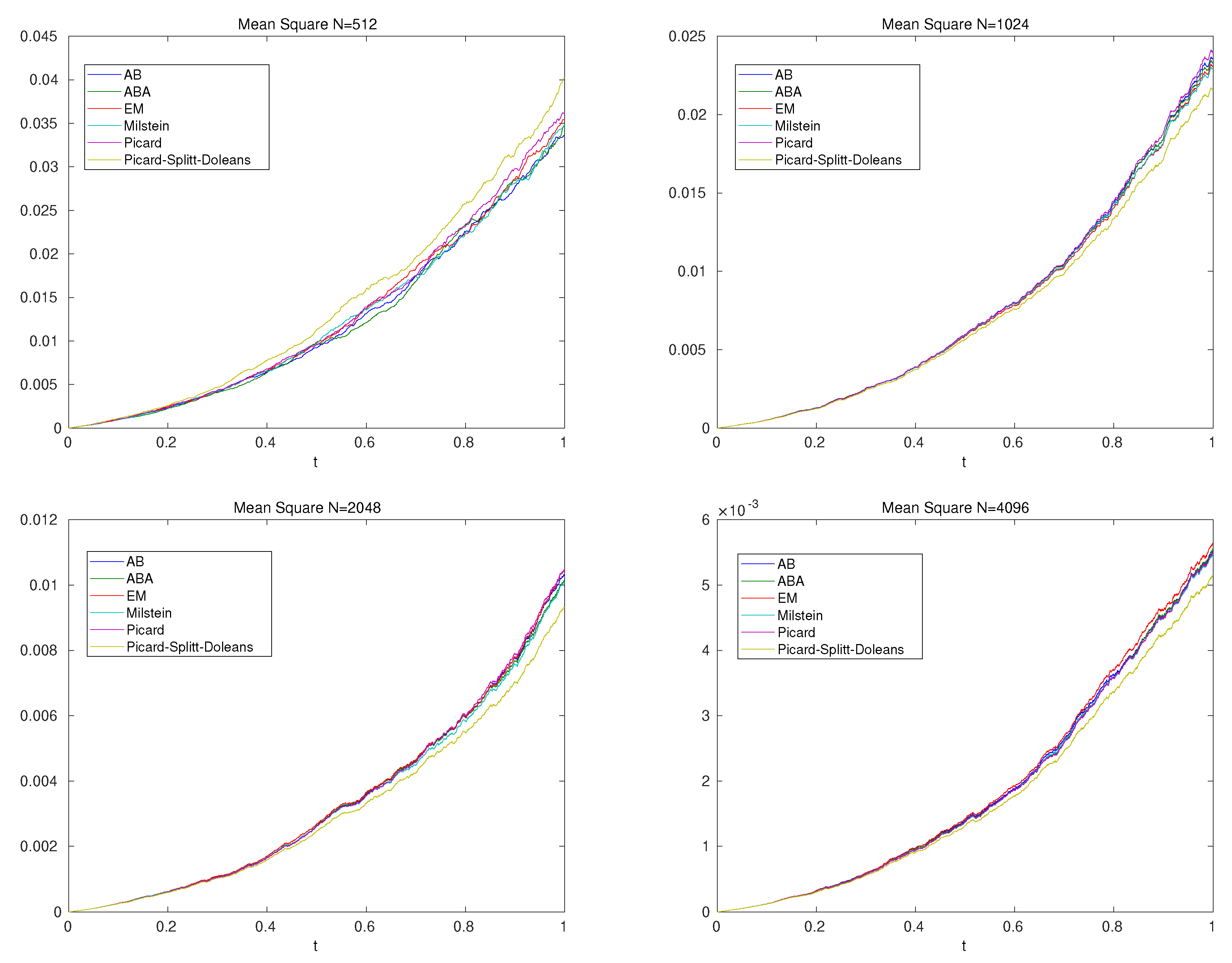
• Mean value at $t=t^n$ and J-sample paths:

  $$\begin{array}{c}\hfill E(X_{method}(t_n))=\frac{1}{J}\sum _{j=1}^J{X}_{method}^j(t_n),\end{array}$$

  (29)

  we deal with time-step $\Delta t=\frac{1}{N}$ with $N=512,1024,2048,4096$ and the time-points are $t_n$, $n=1,\dots ,N$ with end-time-point $t_N=1.0$. For the sample paths, we apply $J=100$ or $J=1000$ and for the methods, we have $method=\{AB,ABA,Em,Mil,Picard,Picard-Doleans,Picard-Splitt-Doleans\}$.
• Local mean square error value at $t=t_n$ and J-sample paths:

  $$\begin{array}{c}Var{(X_{method}(t_n))}_{local}=\frac{1}{J}\sum _{j=1}^J{|E(X_{method}(t_n))-X_{method}^j(t_n)|}^2,\hfill \end{array}$$

  (30)

  we deal with time-step $\Delta t=\frac{1}{N}$ with $N=512,1024,2048,4096$ and the time-points are $t_n$, $n=1,\dots ,N$ with end-time-point $t_N=1.0$. For the sample paths, we apply $J=100$ or $J=1000$ and for the methods, we have $method=\{AB,ABA,Em,Mil,Picard,Picard-Doleans,Picard-Splitt-Doleans\}$.
• Global means square error over the full time-scale with different time-steps $\Delta t$ and J-sample path:

  $$\begin{array}{c}Var{(X_{method})}_{global}=\sum _{n=0}^N\Delta tVar{(X_{method}(t_n))}_{local},\hfill \end{array}$$

  (31)

  where we apply the Equation (30) for the local means square error. Further, we deal with $\Delta t=\frac{1}{N}$ with $N=512,1024,2048,4096$. For the sample paths, we apply $J=100$ or $J=1000$ and for the methods, we have $method=\{AB,ABA,Em,Mil,Picard,Picard-Doleans,Picard-Splitt-Doleans\}$.

Remark 1.

We could reduce the computational time, while we decompose the exp-operator and apply Pade-approximation. We saw in experiments, that we could accelerate the computation of 2–3 times, such that we are in the same region as the ABA-splitting approach, see the remarks in Appendix A.2.

In the following Table 1, we present the means-values at $t=1.0$.

Table 1. Mean values of the all the methods at time-point $t=1.0$.

N	EM-	Milstein	AB	ABA	Picard	Picard-	Picard-Splitt-
						Doleans	Doleans
					$\mathit{i}=\mathbf{2}$	$\mathit{i}=\mathbf{2}$	$\mathit{i}=\mathbf{2}$
$2^9$	$33.9535$	$35.5878$	$35.4419$	$34.6244$	$40.6004$	$37.8312$	$31.3049$
$2^{10}$	$34.4942$	$35.4737$	$34.1016$	$34.529$	$40.0732$	$37.9911$	$32.2207$
$2^{11}$	$34.7694$	$34.2016$	$35.2721$	$34.0984$	$40.6338$	$37.9833$	$30.5993$
$2^{12}$	$34.2202$	$36.2405$	$35.1938$	$35.8434$	$40.1492$	$37.9433$	$31.4823$

In the following Figure 1, we present the exact solution of the first experiment.

Figure 1. The exact solution of the stochastic differential equation (SDE) in the first experiment.

In the following Figure 2, we present the mean value, while we apply Equation (29), with different time-steps and for all numerical methods.

Figure 2. Results of the mean values are computed with Equation (29) and they are presented for the different methods with the following number of time steps $N=512,1024,2048,4096$.

In the following Figure 3, we present the mean square error, while we apply Equation (31), with different time-steps and for all numerical methods.

Figure 3. Results of mean square errors are computed with Equation (31) and they are presented for the different methods with the following number of time steps $N=512,1024,2048,4096$.

In the following Figure 4, we present the performance of the schemes.

Figure 4. Performance of the different schemes, where we compute the mean error values of the different methods at $t=1.0$ with $J=100$ samples and different number of time-steps with $N=500,1000,1500,2000,2500,3000,3500,4000$.

Remark 2.

In the Figure 2 and Figure 3, we present the mean and the mean-square-errors of the different schemes. We see the higher stability and the benefits of the iterative splitting, which applied symmetric techniques like the Doléans-Dade exponential approach. The locally Lipschitz operators are more stable to compute, while we could bound the operators in an exponential-approach, see [12]. In the performance, see Figure 7 in Section 3.2 we see, that the exponential based methods, like the Picard-Doleans or the Picard-Splitt-Doleans, are 2–3 times higher, than the standard schemes. But we obtain much more accurate and stable results and could use much more larger time-steps, such that we accelerate the solver process. Here, the restriction to the CFL-condition for the EM-, Milstein-schemes are higher and therefore the exponential based methods can use larger time-steps or are more accuracy with the same time-steps. For an increasing of the volatility in the stochastic differential equation, we have a stable method based on the Picard-Doleans or Picard-Splitt-Doleans. Here, we deal with an implicit behaviour of the underlying methods and we have to be aware of the numerical diffusion, which appear with larger time-steps, see [30].

3.2. Second Example: Linear/Nonlinear SDE with Potential Function

We deal with a test-example based on root- or irrational functions, see also [29].

The function is given as:

$$\begin{array}{c}dX(t)=(2X^{1/2}+1)dt+2X^{1/2}d{W}_t,t\in \times [0,1],\hfill \end{array}$$

(32)

$$\begin{array}{c}X(0)=1.\hfill \end{array}$$

(33)

The analytical solution can be derived by the Ito-Taylor expansion, see [29] and we obtain:

$$\begin{array}{c}X(t)={\left(X(0)+t+W(t)\right)}^2,\hfill \end{array}$$

where $W(t)=W_t-W_0=\sqrt{t}\xi$ and $\xi$ obeys the Gaussian normal distribution $N(0,1)$ with $E(\xi )=0$ and $E({\xi }^2)=Var(\xi )=1$. $W(t)\approx \sqrt{t}N(0,1)$ and $N(0,1)$ indicates a standard normal random variable.

We deal with the following numerical methods. Further, we apply the time-intervals $\Delta t=\frac{1}{N}$ with $N=2^9,2^{10},2^{11},2^{12},2^{13}$.

• Euler-Maruyama-Scheme

  $$\begin{array}{c}X(t_{i+1})=X(t_i)+\left(2X^{1/2}(t_i)+1\right)\Delta t+2X^{1/2}(t_i)\Delta W_t,\hfill \end{array}$$

  where $\Delta t=t_{i+1}-t_i$, $\Delta W_t=W_{t_{i+1}}-W_{t_i}=\sqrt{\Delta t}\xi$ and $\xi$ obeys the Gaussian normal distribution $N(0,1)$ with $E(\xi )=0$ and $E({\xi }^2)=Var(\xi )=1$.
  We have $i=0,\dots ,N-1$ with $X(t_0)=1.0$.
• Milstein-Scheme

  $$\begin{array}{c}X(t_{i+1})=X(t_i)+\left(2X^{1/2}(t_i)+1\right)\Delta t+2X^{1/2}(t_i)\Delta W_t+\frac{1}{2}({(\Delta W_t)}^2-\Delta t),\hfill \end{array}$$

  where $\Delta t=t_{i+1}-t_i$, $\Delta W_t=W_{t_{i+1}}-W_{t_i}=\sqrt{\Delta t}\xi$ and $\xi$ obeys the Gaussian normal distribution $N(0,1)$ with $E(\xi )=0$ and $E({\xi }^2)=Var(\xi )=1$.
  We have $i=0,\dots ,N-1$ with $X(t_0)=1.0$.
• AB-splitting approach:
  We initialize $t_i$ with $i=0,\dots ,N-1$, while $t_N=T$ and we have $X(0)$ is the initial condition.
  We deal with the 2 steps:
  • A-step:

    $$\begin{array}{c}\tilde{X}(t_{i+1})=X(t_i)+\left(2X^{1/2}(t_i)+1\right)\Delta t,\hfill \end{array}$$
  • B-part:

    $$\begin{array}{c}X(t_{i+1})=\tilde{X}(t_{i+1})+2{\tilde{X}}^{1/2}(t_{i+1})\Delta W_t+\frac{1}{2}({(\Delta W_t)}^2-\Delta t),\hfill \end{array}$$

    where we have the solution $X(t_{i+1})$ and we go to the next time-step till $i=N-1$.
• ABA-splitting approach:
  We initialize $t_i$ with $i=0,\dots ,N-1$, while $t_N=T$ and we have $X(0)$ is the initial condition.
  We deal with the 2 steps:
  • A-step ($\Delta t/2$):

    $$\begin{array}{c}\hfill \tilde{X}(t_{i+1})=X(t_i)+\left(2X^{1/2}(t_i)+1\right)\Delta t/2,\end{array}$$
  • B-part ($\Delta t$):

    $$\begin{array}{c}\widehat{X}(t_{i+1})=\tilde{X}(t_{i+1})+2{\tilde{X}}^{1/2}(t_{i+1})\Delta W_t+2({(\Delta W_t)}^2-\Delta t),\hfill \end{array}$$
  • A-step ($\Delta t/2$):

    $$\begin{array}{c}\hfill X(t_{i+1})=\widehat{X}(t_{i+1})+\left(2{\widehat{X}}^{1/2}(t_{i+1})+1\right)\Delta t/2,\end{array}$$

    where we have the solution $X(t_{i+1})$ and we go to the next time-step till $i=N-1$.
• Iterative Picard approach:

  $$\begin{array}{c}dX(t)=(2X^{1/2}+1)dt+2X^{1/2}d{W}_t,t\in \times [0,1],\hfill \\ X(0)=1,\hfill \end{array}$$

  we apply an Picard-Iteration

  $$\begin{array}{c}d{X}_i(t)=(2X_{i-1}^{1/2}+1)dt+2X_{i-1}^{1/2}d{W}_t,t\in \times [0,1],\hfill \\ X(0)=1,\hfill \end{array}$$

  where $X_0(t)=x(0)$, while we apply the implicit method for the drift term and the explicit method for the diffusion term.
  The algorithm is given as:
  We initialize $t_n$ with $n=0,\dots ,N-1$, while $t_N=T$ and we have $X(0)$ is the initial condition.
  We deal with the 2 loops (loop 1 is the computation over the full time-domain and loop 2 is the computation with $i=1,2,\dots$):
  • $n=0,\dots ,N-1$:
  • $i=1,\dots ,I$:
  • Computation

    $$\begin{array}{c}{X}_i(t^{n+1})=X(t^n)+(2X_{i-1}{(t^{n+1})}^{1/2}+1)\Delta t\hfill \\ +2X^{1/2}(t^n)\Delta W_t+\frac{1}{2}({(\Delta W_t)}^2-\Delta t),t\in \times [0,1],\hfill \\ X(0)=1,\hfill \end{array}$$

    where $\Delta t=t^{n+1}-t^n$, $\Delta W_t=W_{t^{n+1}}-W_{t^n}=\sqrt{\Delta t}\xi$ and $\xi$ obeys the Gaussian normal distribution $N(0,1)$ with $E(\xi )=0$ and $E({\xi }^2)=Var(\xi )=1$.
  • $i=i+1$, if $i=I+1$ then we are done, else we go to Step (c)
  • $n=n+1$, if $n+1=N+1$ then we are done, else we go to Step (b)
• Iterative Picard-splitting with Doléans-Dade exponential approach:

  $$\begin{array}{c}dX(t)=(2X^{1/2}+1)dt+2X^{1/2}d{W}_t,t\in \times [0,1],\hfill \\ X(0)=1,\hfill \end{array}$$

  we apply the following splitting approach:

  $$\begin{array}{c}A(X(t))=2X^{1/2}+1,\hfill \\ A_1(X(t))=2X^{1/2},A_2(X(t))=1,\hfill \end{array}$$

  where $a_1(X(t))=2X^{-1/2}(t)$.
  We apply an Picard with Doléans-Dade exponential approach and right hand side

  $$\begin{array}{c}d{X}_i(t)=(2X_{i-1}^{-1/2})X_{i}dt+2X_{i-1}^{-1/2}{X}_{i}d{W}_t+1dt,t\in \times [0,1],\hfill \\ X(0)=1,\hfill \end{array}$$

  where $X_0(t)=x(0)$, while we apply the implicit method in the drift term and the explicit method in the diffusion term.
  The algorithm is given as: We initialize $t_n$ with $n=0,\dots ,N-1$, while $t_N=T$ and we have $X(0)$ is the initial condition.
  We deal with the 2 loops (loop 1 is the computation over the full time-domain and loop 2 is the computation with $i=1,2,\dots$):
  • $n=0,\dots ,N-1$:
  • $i=1,\dots ,I$:
  • Computation (we apply Version 1 or Version 2)
  • Computation (we apply the full exp and integration of the RHS)

    $$\begin{array}{c}X{(t_{n+1})}^i=X(t_n)exp(\Delta t\frac{\left(2X^{-1/2}{(t_{n+1})}^{i-1}+2X^{-1/2}(t_n)\right)}{2}\hfill \\ -\Delta t\frac{\left(X^{-1}{(t_{n+1})}^{i-1}+X^{-1}(t_n)\right)}{2}\hfill \\ +2X^{-1/2}(t_n)\Delta W_t+\frac{1}{2}{X}^{-1}(t_n)({(\Delta W_t)}^2-\Delta t))+\Delta t.\hfill \end{array}$$

    (34)
  • $i=i+1$, if $i=I+1$ then we are done, else we go to Step (c)
  • $n=n+1$, if $n+1=N+1$ then we are done, else we go to Step (b)

We obtain a critical CFL condition, given as following:

$$\begin{array}{c}\Delta t\le \frac{X}{4{\xi }^2},\hfill \end{array}$$

(35)

where $\xi$ is $N(0,1)$ distributed. If the criterion is done all is fine and we go on. If we reach such a value, we reduce the time-step $\Delta t$ for the recent time step to $\Delta t=\frac{X}{4{\xi }^2}$. For the next time-step, we could use the old time step and so on.

Remark 3.

In the mixed example with additional right hand side, we could reduce the computational time, while we decompose into symmetric operators. We have applied an exp-operator and via Taylor- or Pade-approximation and additional a convolution operator with the right-hand side, see also [12]. We saw the stable behaviour of such a splitting and could additionally accelerate the computation of 2–3 times, such that we are in the same region as the ABA-splitting approach, see the remarks in Appendix A.2.

In the following Figure 5, we present the mean value, which is computed with the Equation (29) with different time-steps and for all the numerical methods.

Figure 5. Results of the mean values, which are computed with Equation (29) and they are presented for the different methods with the number of time steps $N=512,1024,2048,4096$.

In the following Figure 6, we present the mean square error, which is computed with the Equation (31) with different time-steps and for all the numerical methods.

Figure 6. Results of mean square errors, which are computed with Equation (31) and they are presented for the different methods with the number of time steps $N=512,1024,2048,4096$.

In the following Figure 7, we present the performance of the schemes.

Figure 7. Performance of the different schemes, where we compute the mean error values of the different methods at $t=1.0$ with $J=100$ samples and different number of time-steps with $N=500,1000,1500,2000,2500,3000,3500,4000$.

Remark 4.

In the second example, which is a mixed linear and nonlinear stochastic differential equation, we also see the benefit and the efficiency of the iterative splitting approaches with Doléans-Dade exponential approach. Based on the local Lipschitzian of the coefficients, we could also apply larger timesteps for the exponential method with an iterative method. Such a Picard iterations solve the nonlinear parts of the operators and we could stabilize the nonlinear growth-parts with the exponential exponential approach. This allows to neglect the blow-ups in the exponential growth with sufficient large time-steps, see [10,16]. Further the benefit in splitting into symmetric parts of nonlinear and linear parts allows to accelerate the solver processes, see [31]. The benefit of larger time-steps for the iterative Picard-splitting with Doléans-Dade exponential approach can also applied to increasing volatilities in the SDEs. Here, we have to consider the implicit character of the iterative Picard-splitting approaches, see [30]. Such a behaviour can smear or smoothen out the solution of increasing volatility, like increasing diffusion, such that it might be necessary to apply multiscale methods with much more finer time-steps or an restriction of the time-step around the CFL-condition, see [30,32].

4. Conclusions

We have discussed a new iterative splitting approach, which is based on Picard iterations and Doléans-Dade exponential approach. We proof the convergence of such new schemes, which have embedded the Doléans-Dade exponential approach. Such a combinations allow to circumvent the global non-Lipschitz problems and therefore consider more stable local Lipschitz problems. Such a local problem can be solved with reformulations of exponential based operators, which are more stable in the numerical approach. We could embed such locally Lipschitz problems into a splitting approach which deals with exponential parts and a nonlinear solver given as Picard’s method. Such a combination allows to obtain stable and convergent methods. Due to symmetric approaches of the operators, we could split into more appropriate linear, nonlinear and stochastic operators, which allows faster computations. The first numerical results are tested with linear and nonlinear stochastic differential equations with rational functions of the drift and diffusion parts. We present the benefits of the iterative splitting approach with the Doléans-Dade exponential, while we obtain an implicit method with stable results. Therefore, we are independent of the CFL conditions and accelerate the solver process. In future, we will test the splitting approach to more inhomogeneous problems and in the case of increasing volatility, e.g., real-life problems with stochastic lubrication models.

Appendix A.1. Additional Proofs

We have the Lemma A1 as following; see also the proof in paper [5].

Lemma A1.

We have $f^m(t)$ be a sequence of positive functions, which are defined on the interval $t\in [0,T]$, with $T>0$, such that we have for some $C>0$:

$$\begin{array}{c}\hfill f^{m+1}(t)\le C{\int }_0^t{g}^m(s)ds,0\le f^0\le C,\end{array}$$

(A1)

then we obtain:

$$\begin{array}{c}\hfill \underset{t\in [0,T]}{sup}{f}^{m+1}(t)\le C^m\frac{t^m}{m!}\underset{t\in [0,T]}{sup}{f}^0(t).\end{array}$$

(A2)

Proof. 

The proof is sketch as following, see also [5]: We can bound the function $g^0$ as:

$$\begin{array}{c}\hfill C_f:=\underset{t\in [0,T]}{sup}{f}^0(t)\le C.\end{array}$$

We apply:

$$\begin{array}{c}\hfill \underset{t\in [0,T]}{sup}{f}^{m-1}(t)\le C^{m-1}\frac{t^{m-1}}{(m-1)!}{C}_f,\end{array}$$

then we can apply the integral an obtain

$$\begin{array}{c}\hfill f^m(t)\le C{\int }_0^t{C}^{m-1}\frac{s^{m-1}}{(m-1)!}{C}_{f}ds.\end{array}$$

By integration, we receive the results, that proves our lemma. □

Appendix A.2. Approximated exp-Functions

We can reduce the computational time for the Doléans-Dade exponential approach with the following reductions:

• Version with reduced $exp$ in Example 1: We replace the Equation (27) with the reduced exponential function, see:

  $$\begin{array}{c}\hfill \begin{array}{c}X{(t_{n+1})}^i=\left(X(t_n)+\Delta t\frac{2}{5}\frac{\left(X^{-2/5}{(t_{n+1})}^{i-1}+X^{-2/5}(t_n)\right)}{2}\right)\hfill \\ ·(1+\Delta t5\frac{\left(X^{-1/5}{(t_{n+1})}^{i-1}+X^{-1/5}(t_n)\right)}{2}-\Delta t\frac{1}{2}\frac{\left(X^{-2/5}{(t_{n+1})}^{i-1}+X^{-2/5}(t_n)\right)}{2}\hfill \\ +X^{-1/5}(t_n)\Delta W_t+\frac{1}{2}{X}^{-2/5}(t_n)({(\Delta W_t)}^2-\Delta t)),\hfill \end{array}\end{array}$$

  (A3)

  where we assume to choose and appropriate $\Delta t>0$ with $\left(1+\Delta t5\frac{\left(X^{-1/5}{(t_{n+1})}^{i-1}+X^{-1/5}(t_n)\right)}{2}-\Delta t\frac{1}{2}\frac{\left(X^{-2/5}{(t_{n+1})}^{i-1}+X^{-2/5}(t_n)\right)}{2}+X^{-1/5}(t_n)\Delta W_t+\frac{1}{2}{X}^{-2/5}(t_n)({(\Delta W_t)}^2-\Delta t)\right)\ge 0$.
• Version with reduced $exp$ in Example 2: We replace the Equation (34) with the reduced exponential function and integration of the RHS, see:

  $$\begin{array}{c}X{(t_{n+1})}^i=X(t_n)(1+\Delta t\frac{\left(2X^{-1/2}{(t_{n+1})}^{i-1}+2X^{-1/2}(t_n)\right)}{2}\hfill \\ -\Delta t\frac{\left(1X^{-1}{(t_{n+1})}^{i-1}+1X^{-1}(t_n)\right)}{2}\hfill \\ +2X^{-1/2}(t_n)\Delta W_t+\frac{1}{2}{X}^{-1}(t_n)({(\Delta W_t)}^2-\Delta t))+\Delta t.\hfill \end{array}$$

  (A4)

References

- Zhang, Z.; Karniadakis, G.E. Numerical Methods for Stochastic Partial Differential Equations with White Noise; Applied Mathematical Sciences, No. 196; Springer International Publishing: Heidelberg/Berlin, Germany; New York, NY, USA, 2017. [Google Scholar]
- Duran-Olivencia, M.A.; Gvalani, R.S.; Kalliadasis, S.; Pavliotis, G.A. Instability, Rupture and Fluctuations in Thin Liquid Films: Theory and Computations. arXiv 2017, arXiv:1707.08811. [Google Scholar] [CrossRef] [PubMed]
- Grün, G.; Mecke, K.; Rauscher, M. Thin-film flow influenced by thermal noise. J. Stat. Phys. 2006, 122, 1261–1291. [Google Scholar] [CrossRef]
- Diez, J.A.; González, A.G.; Fernández, R. Metallic-thin-film instability with spatially correlated thermal noise. Phys. Rev. E Am. Phys. Soc. 2016, 93, 013120. [Google Scholar] [CrossRef] [PubMed]
- Baptiste, J.; Grepat, J.; Lepinette, E. Approximation of Non-Lipschitz SDEs by Picard Iterations. J. Appl. Math. Financ. 2018, 25, 148–179. [Google Scholar] [CrossRef]
- Geiser, J. Multicomponent and Multiscale Systems: Theory, Methods, and Applications in Engineering; Springer: Heidelberg, Germany, 2016. [Google Scholar]
- Moler, C.B.; Loan, C.F.V. Nineteen dubious ways to compute the exponential of a matrix, twenty-five years later. SIAM Rev. 2003, 45, 3–49. [Google Scholar] [CrossRef]
- Bader, P.; Blanes, S.; Fernando, F.C. Computing the Matrix Exponential with an Optimized Taylor Polynomial Approximation. Mathematics 2019, 7, 1174. [Google Scholar] [CrossRef]
- Najfeld, I.; Havel, T.F. Derivatives of the matrix exponential and their computation. Adv. Appl. Math. 1995, 16, 321–375. [Google Scholar] [CrossRef]
- Geiser, J. Iterative semi-implicit splitting methods for stochastic chemical kinetics. In Proceedings of the Seventh International Conference, FDM:T&A 2018, Lozenetz, Bulgaria, 11–26 June 2018; Lecture Notes in Computer Science No. 11386: 32-43. Springer: Berlin/Heidelberg, Germany, 2018. [Google Scholar]
- Geiser, J.; Bartecki, K. Iterative and Non-iterative Splitting approach of the stochastic inviscid Burgers’ equation. In Proceedings of the AIP Conference Proceedings Paper, ICNAAM 2019, Rhodes, Greece, 23–28 September 2019. [Google Scholar]
- Geiser, J. Iterative Splitting Methods for Differential Equations; Numerical Analysis and Scientific Computing Series; Taylor & Francis Group: Boca Raton, FL, USA; London, UK; New York, NY, USA, 2011. [Google Scholar]
- Geiser, J. Additive via Iterative Splitting Schemes: Algorithms and Applications in Heat-Transfer Problems. In Proceedings of the Ninth International Conference on Engineering Computational Technology, Naples, Italy, 2–5 September 2014; Ivanyi, P., Topping, B.H.V., Eds.; Civil-Comp Press: Stirlingshire, UK, 2014. [Google Scholar] [CrossRef]
- Vandewalle, S. Parallel Multigrid Waveform Relaxation for Parabolic Problems; Teubner Skripten zur Numerik, B.G. Teubner Stuttgart: Leipzig, Germany, 1993. [Google Scholar]
- Gyöngy, I.; Krylov, N. On the Splitting-up Method and Stochastic Partial Differential Equations. Ann. Probab. 2003, 31, 564–591. [Google Scholar] [CrossRef]
- Duan, J.; Yan, J. General matrix-valued inhomogeneous linear stochastic differential equations and applications. Stat. Probab. Lett. 2008, 78, 2361–2365. [Google Scholar] [CrossRef]
- Bonaccorsi, S. Stochastic variation of constants formula for infinite dimensional equations. Stoch. Anal. Appl. 1999, 17, 509–528. [Google Scholar] [CrossRef]
- Reiss, M.; Riedle, M.; van Gaans, O. On Emery’s Inequality and a Variation-of-Constants Formula. Stoch. Anal. Appl. 2007, 25, 353–379. [Google Scholar] [CrossRef]
- Scheutzow, M. Stochastic Partial Differential Equations; Lecture Notes, BMS Advanced Course; Technische Universität Berlin: Berlin, Germany, 2019; Available online: http://page.math.tu-berlin.de/~scheutzow/SPDEmain.pdf (accessed on 20 February 2020).
- Prato, G.D.; Jentzen, A.; Röckner, M. A mild Ito formula for SPDEs. Trans. Am. Math. Soc. 2019, 372, 3755–3807. [Google Scholar] [CrossRef]
- Deck, T. Der Ito-Kalkül: Einführung und Anwendung; Springer: Berlin/Heidelberg, Germany, 2006. [Google Scholar]
- Teschl, G. Ordinary Differential Equations and Dynamical Systems; American Mathematical Society, Graduate Studies in Mathematics: Providence, RI, USA, 2012; Volume 140. [Google Scholar]
- Oksendal, B. Stochastic Differential Equations: An Introduction with Applications; Springer: Heidelberg/Berlin, Germany, 2003. [Google Scholar]
- Stoer, J.; Bulirsch, R. Introduction to Numerical Analysis; Springer: Heidelberg/Berlin, Germany; New York, NY, USA, 1980. [Google Scholar]
- Kloeden, P.E.; Platen, E. The Numerical Solution of Stochastic Differential Equations; Springer: Berlin/Heidelberg, Germany, 1992. [Google Scholar]
- Karlsen, K.H.; Storrosten, E.B. On stochastic conservation laws and Malliavin calculus. J. Funct. Anal. 2017, 272, 421–497. [Google Scholar] [CrossRef]
- Ninomiya, S.; Victoir, N. Weak approximation of stochastic differential equations and application to derivative pricing. Appl. Math. Financ. 2008, 15, 107–121. [Google Scholar] [CrossRef][Green Version]
- Ninomiya, M.; Ninomiya, S. A new higher-order weak approximation scheme for stochastic differential equations and the Runge–Kutta method. Financ. Stoch. 2009, 13, 415–443. [Google Scholar] [CrossRef]
- Bayram, M.; Partal, T.; Buyukoz, G.O. Numerical methods for simulation of stochastic differential equations. Adv. Differ. Equ. 2018, 2018. [Google Scholar] [CrossRef]
- Geiser, J. Multicomponent and Multiscale Systems—Theory, Methods, and Applications in Engineering; Springer International Publishing AG: Heiderberg/Berlin, Germany; New York, NY, USA, 2016. [Google Scholar]
- Geiser, J. Computing Exponential for Iterative Splitting Methods: Algorithms and Applications. Math. Numer. Model. Flow Transp. 2011, 2011, 193781. [Google Scholar] [CrossRef]
- Fouque, J.-P.; Papanicolaou, G.; Sircar, R. Multiscale Stochastic Volatility Asymptotics. SIAM J. Multiscale Model. Simul. 2003, 2, 22–42. [Google Scholar] [CrossRef]
© 2020 by the author. Licensee MDPI, Basel, Switzerland. This article is an open access article distributed under the terms and conditions of the Creative Commons Attribution (CC BY) license (http://creativecommons.org/licenses/by/4.0/).