A Kinematic Calibration Method of a 3T1R 4-Degree-of-Freedom Symmetrical Parallel Manipulator

Abstract

This paper proposes a method for kinematic calibration of a 3T1R, 4-degree-of-freedom symmetrical parallel manipulator driven by two pairs of linear actuators. The kinematic model of the individual branched chain is established by using the local product of exponentials formula. Based on this model, the model of the end effector’s pose error is established from a pair of symmetrical branched chains, and a recursive least square method is applied for the parameter identification. By installing built-in sensors at the passive joints, a calibration method for a serial manipulator is eventually extended to this parallel manipulator. Specifically, the sensor installed at the second revolute joint of each branched chain is saved, replaced by numerical calculation according to kinematic constraints. The simulation results validate the effectiveness of the proposed kinematic error modeling and identification methods. The procedure for pre-processing compensation on this 3T1R parallel manipulator is eventually given to improve its absolute positioning accuracy, using the inverse of the calibrated kinematic model.

1. Introduction

Compared with serial manipulators, parallel manipulators have the advantages of high rigidity and high loading capacity [1], but also have the disadvantages of complex structure and relatively small workspace. Recently, a 3T1R symmetrical parallel manipulator with a simple structure and a large working space has received widespread attention in academia and industrial applications [2]. This symmetrical parallel manipulator uses four open branched chains to connect the fixed platform with the moving platform. It can achieve three-degree-of-freedom translation along the X, Y, and Z axes and one-degree-of-freedom rotation around the Z axis (3T1R), for a total of four degrees of freedom. Its advantages such as large workspace and high speed make it be widely applicable to industrial automation scenarios such as pick-and-place and sorting, if its absolute positioning accuracy meets the particular requirements of these applications. Therefore, it is necessary to develop an effective calibration method to improve the absolute positioning accuracy of this symmetrical parallel manipulator [3,4].

The kinematic error of the manipulator is defined as the end effector’s error between the actual pose and the nominal one, which is mainly caused by geometric tolerances, such as assembly and manufacturing error. Kinematic calibration is the most effective and economical method to improve accuracy [5]. This method is generally divided into four steps. First is to establish a kinematic error model that consists of parameters to be identified and the measurable variables. Second is to acquire measurements from built-in or external sensors. Third is to perform the identification of parameters in the error model. Fourth is to carry out simulation verification of the calibrated kinematic model and to perform relevant calibration experiments [6,7].

Establishing a proper kinematic error model is the basis for parallel manipulator calibration. The essence of this process is the mapping between the pose error of the moving platform and the error source [8]. Although many modeling methods involving parallel manipulators have been proposed, the modeling method of kinematic error for such a 3T1R complex symmetrical parallel manipulator has not been mentioned yet. Compared with traditional manipulators’ calibration methods such as the Denavit–Hartenberg (D-H) model based method [9] and the zero-position reference model method [10], the error model based on the local product of exponentials (POE) formula has some advantages [11,12]. First, the parameters of the kinematic model on the POE formula change smoothly with the change of the joint axis. This ensures that the singularity will not occur in the kinematic error model [11,13]. Secondly, according to Chase’s theorem, any rigid body motion can be regarded as a screw motion, so the calibration model established by the POE formula is also complete [14]. Last but not least, on the POE formula, all joint axes are described based on Lie geometry, so they are represented uniformly for the translation and rotation joints of the robot [14].

Since Okamura and Park first introduced the POE formula to robotic kinematics calibration in 1996 [13], the establishment of a kinematic error model using the POE formula has received widespread attention. Two ways have been proposed till now, using the global POE formula [14,15] or the local POE formula [11,16]. The main difference between them is on the choice of reference frames to describe the relative motion of the robot joints. In the global POE formula, the relative motion of the robot joints is described in the base coordinate system. In the local POE formula, each link of the robot is assigned a local coordinate system, and all joint motions are expressed in the corresponding local coordinate system. The main advantage of building the kinematic error model using the local POE formula is that the pose error of the end effector is considered to be solely caused by the accumulation of the pose error of each link.

The accuracy of measurement has a great impact on the calibration. Various devices have been used to perform the calibration experiments on parallel manipulators, such as the ball and stick system [17], the magnetic processing ball [18], vision [19], the laser tracker [20], etc. Since there are multiple passive joints in the 3T1R parallel manipulator, installation of sensors on every passive joint for calibration purposes will be costly. The identification of the kinematic error model parameters is performed by minimizing the deviation between the theoretical and measured values of kinematic error, such as nonlinear least squares optimization [21], but the optimization efficiency may be low due to the nonlinear nature of the model. The error pre-processing compensation will be performed after obtaining the kinematic error model. This step is to use the identified parameters to modify the active joint variables, so that the absolute positioning accuracy of the parallel manipulator is enhanced [22].

The 3T1R parallel manipulator has a “two-layer, binary-tree”-like symmetrical mechanism, while symmetry issues have received widespread attention in academia [23,24,25]. In this paper, the development of its kinematic calibration method is studied. Its symmetrical structure leads to the establishment of the kinematic model and the associated error model from two branched chains symmetrically. In detail, the local POE formula method is used for modeling its kinematic error firstly. This approach attributes the errors to the initial pose of each joint, resulting in a simpler kinematic error model. In addition, this work uses the pose of the end effector from two branched chains to evaluate the kinematic error. Compared with the kinematic error modeling methods using the metric of the distance of two points on the end effector [26,27], setting up the equality of pose errors from two branched chains improves the error model fitness. In the measurement stage, a method of combining a built-in sensor with an external measurement device is adopted. Although this 3T1R parallel manipulator has multiple passive joints, all of them can be treated as active ones as in the series robot, if sensors are attached to them during calibration. In this way, the calibration method by the local POE formula used for serial robots can be directly applied to parallel manipulators with passive joints. Specifically, to save the number of sensors used in the revolute joints, the angle of the second revolute joint of each branched chain is computed numerically according to the kinematic constraints of the mechanism. Eventually, a linear-in-parameter error model is synthesized, which greatly improves the efficiency in the coming least squares estimation of parameters. Due to the symmetry of this mechanism, the idle pair of branched chains can be used for cross-validation of the kinematic and error models, thereby ensuring the model accuracy. A simulation study of the calibration algorithm is performed to verify the effectiveness of the algorithm. Last but not least, the pre-processing compensation procedure of the command pose is suggested for this 3T1R parallel manipulator.

2. Kinematics of a Symmetrical 3T1R Parallel Manipulator

In order to establish a kinematic model for the symmetrical 3T1R parallel manipulator, the basic structure of this parallel manipulator is firstly introduced. Subsequently, its forward kinematics based on the local POE formula is derived. It lays the foundation for the subsequent establishment of the kinematic error model for this parallel manipulator.

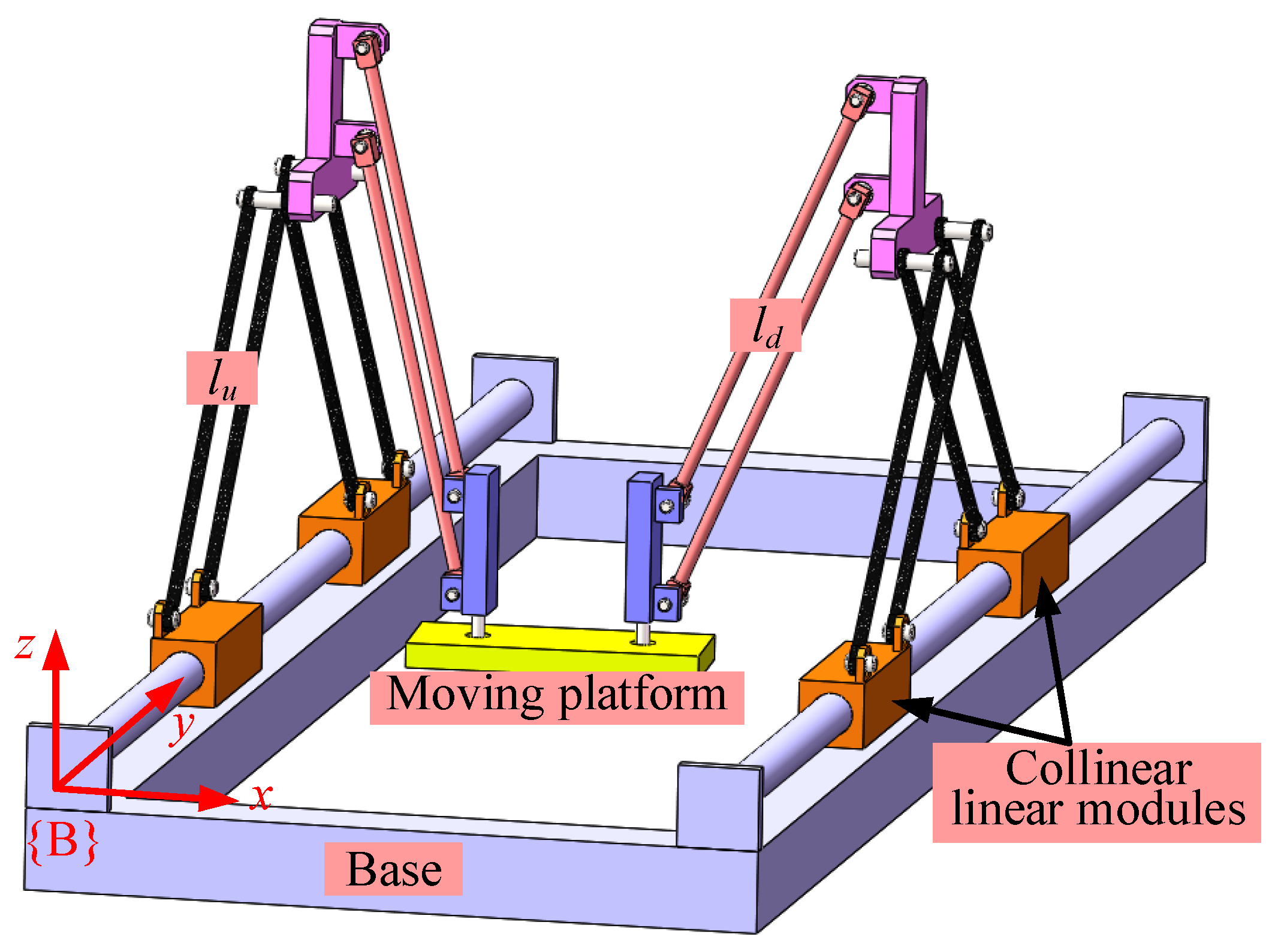
2.1. Structure of the 3T1R Parallel Manipulator

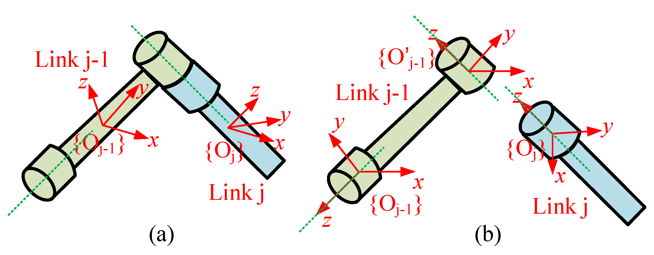
As shown in Figure 1, it has two identical branched chains, yielding symmetrical structures. Each branched chains has two identical sub-branches, so the whole mechanism can be treated as a “binary-tree” structure. This parallel manipulator is driven by four linear actuators installed on the base, and two linear actuators on one side share one stator. The entire manipulator mechanism looks like the shape of the letter “M”, and it can move along the X, Y, and Z axes and rotate about the Z axis.

2.2. $Dyad$ kinematics Based on local POE formula

The $Dyad$ branched chain is shown in Figure 2. Based on the traditional local POE formula method of building in Figure 2a, the $Dyad$ kinematics can be obtained as (1):

$$\begin{array}{c}\hfill T_{j-1,j}=T_{j-1}\left(0\right)·e^{{\widehat{s}}_j{q}_j},\end{array}$$

(1)

where $T_{j-1,j}\in SE\left(3\right)$, represents the pose of $\left\{O_j\right\}$ relative to $\left\{O_{j-1}\right\}$ and uses the representation method of the local coordinate system. ${\widehat{s}}_j$ is the corresponding element for $T_{j-1,j}$ in $se\left(3\right)$.

According to the characteristics of the local POE formula, it is known that the local coordinate system of the POE formula can be assigned arbitrarily, that is the pose of $\left\{O_j\right\}$ is arbitrary, so it requires 13 parameters to completely define $T_{j-1,j}$. Among them, the 13 parameters include: 6 parameters within initial pose $T_{j-1}\left(0\right)\in SE\left(3\right)$, 6 parameters within joint twist ${\widehat{s}}_j\in se\left(3\right)$, and 1 parameter within joint variable $q_j\in R^{1X1}$. Compared with the D-H method, which only needs four parameters to define the kinematics, this method of establishing the kinematic model requires too many parameters.

In order to reduce the number of parameters in the kinematic model, a new method of assigning the local coordinate systems is proposed, as shown in Figure 2b. In this method, the origin of the coordinate system $\left\{O_{j-1}\right\}$ is at the center of the joint, and the direction of the z axis is along the joint line. Furthermore, an additional local coordinate system $\left\{O_{j-1}^{\prime }\right\}$ is on the same link at the joint j. Now, (1) is written as:

$$\begin{array}{c}\hfill T_{j-1,j}=T_{j-1,j}\left(0\right)·e^{{\widehat{s}}_j{q}_j},\end{array}$$

(2)

where $T_{j-1,j}\left(0\right)$ represents the pose transformation of $\left\{O_{j-1}^{\prime }\right\}$ relative to $\left\{O_{j-1}\right\}$. $e^{{\widehat{s}}_j{q}_j}$ represents the pose transformation of $\left\{O_j\right\}$ relative to $\left\{O_{j-1}^{\prime }\right\}$.

According to the transformation between Lie groups and Lie algebras, $T_{j-1,j}\left(0\right)\in SE\left(3\right)$, at least one ${\widehat{t}}_j\in se\left(3\right)$ exists, making $T_{j-1,j}\left(0\right)\in SE\left(3\right)$. Therefore, $T_{j-1,j}\left(0\right)=e^{{\widehat{t}}_j}$, and (2) is written as:

$$\begin{array}{c}\hfill T_{j-1,j}=e^{{\widehat{t}}_j}·e^{{\widehat{s}}_j{q}_j},\end{array}$$

(3)

2.3. Branched Chain Kinematics Based on the Local POE Formula

Based on (2), consider a single branched chain of the parallel manipulator with $(n+1)$ links, numbered sequentially in the order $0, 1, 2\cdots , n$ from base coordinate system $\left\{0\right\}$ to tool coordinate system $\left\{n\right\}$; the forward kinematics is expressed as:

$$\begin{array}{c}\hfill g_{0,n}(q_1,q_2,\dots ,q_n)=T_{0,1}\left(q_1\right)T_{1,2}\left(q_2\right)\dots T_{(n-1),n}\left(q_n\right)=\prod _{i=1}^n\left(T_{(i-1),i}\left(0\right)e^{{\widehat{s}}_i{q}_i}\right).\end{array}$$

(4)

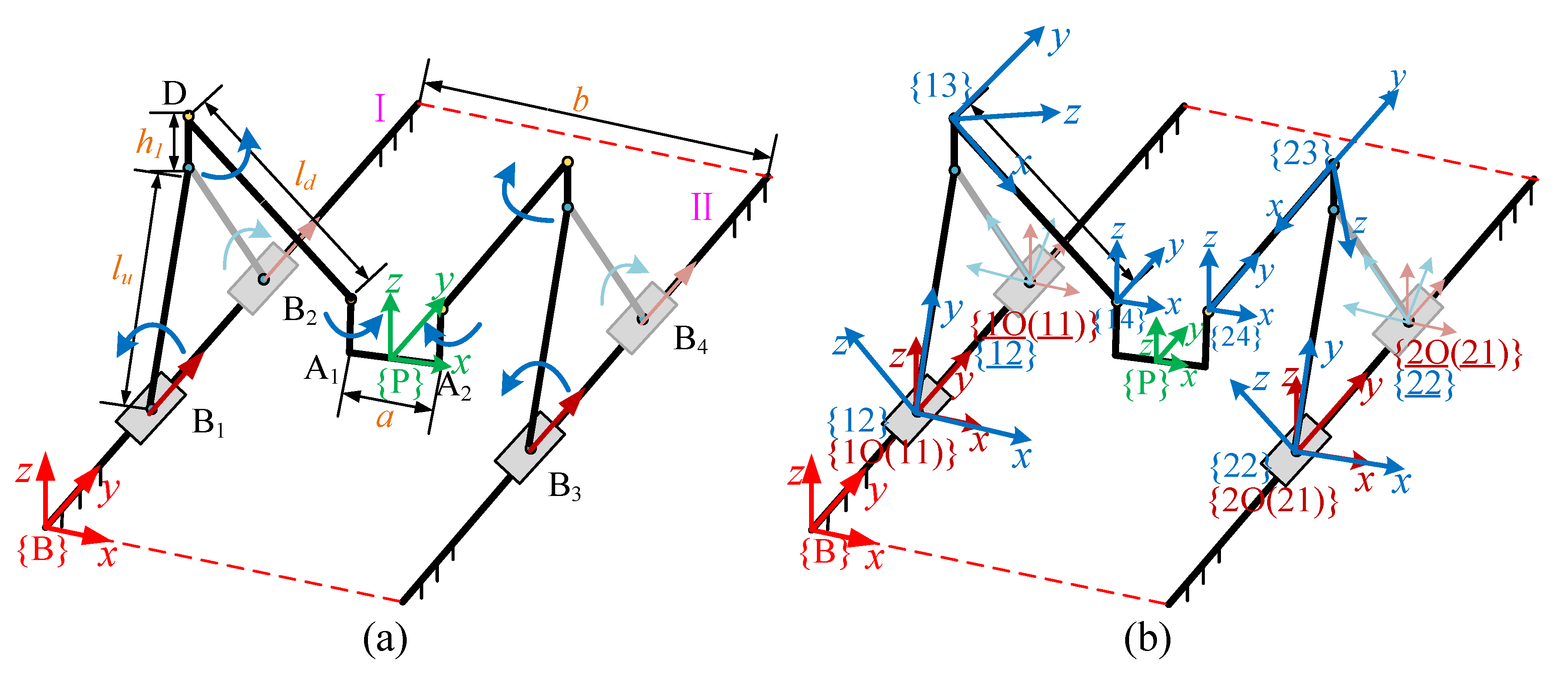
2.4. Kinematics of the Parallel Manipulator Branched Chain i Based on the Local POE Formula

The schematic of the 3T1R parallel manipulator is shown in Figure 3a. It has a symmetrical structure, dividing it into two identical parts, I and II. This parallel manipulator contains four linear actuators $B_1$, $B_2$, $B_3$, and $B_4$. Each linear actuator to the midpoint of the end effector p is regarded as a branched chain. On side I, the branched chains formed by $B_1$ and $B_2$ to the end p point are recorded as i and $\underline{i}$, respectively, where $i=1$; on side II, the branched chains formed by $B_3$ and $B_4$ to the end p point are recorded as i and $\underline{i}$, respectively, where $i=2$. Any one of the branched chains from $B_1$ and $B_2$ and any one from $B_3$ and $B_4$ are chosen to build the entire parallel manipulator kinematics, so there are four possible combinations. In this article, $B_1$ and $B_3$ are chosen for kinematic calibration and recorded as the $i^{\mathrm{th}}$ branched chain, $i=1, 2$, which is the structure indicated by the dark solid line in Figure 1. Surely, because this parallel manipulator structure is symmetrical, the remaining two branch chains can be used to carry out the calibration as well for cross-validation. This also helps to enhance the accuracy of the kinematic model.

There are four joint modules within each branched chain i ($i=1,2$), which are one active translation joint and three passive rotation joints. The coordinate systems are established as shown in Figure 1, and the way of naming is referenced in Nomenclature. The joint $ij$ is an active joint for $i=1, 2$ and j = 1, and the joint $ij$ is a passive joint for $i=1, 2$ and $j=2, 3, 4.$ The pose of the end effector coordinate system $\left\{P\right\}$ relative to the parallel manipulator base coordinate system $\left\{B\right\}$ is defined as the forward kinematics.

The kinematic equation of the mechanism is given as:

$$\begin{array}{c}\hfill g_i=T_{B,i0}·T_{i0,i1}\left(0\right)·e^{{\widehat{s}}_{i1}{q}_{i1}}·T_{i1,i2}\left(0\right)·e^{{\widehat{s}}_{i2}{q}_{i2}}·T_{i2,i3}\left(0\right)·e^{{\widehat{s}}_{i3}{q}_{i3}}·T_{i3,i4}\left(0\right)·e^{{\widehat{s}}_{i4}{q}_{i4}}·T_{i4,P}\left(0\right).\end{array}$$

(5)

3. Establishing the Kinematic Error Model for this 3T1R Parallel Manipulator

Since this parallel manipulator is a closed-chain mechanism, the kinematic error at the end effector of the parallel manipulator should be the same if they are calculated from individual branched chains.

3.1. Establishment of the Kinematic Error Model from a Single Branched Chain

An error model of the 3T1R parallel manipulator, considering the kinematic errors of the single branched chain, is established. Due to the part manufacturing and assembly error, the actual pose of the end effector is different from its nominal value. Since:

$$T_{B,i1}\left(0\right)=T_{B,i0}·T_{i0,11}\left(0\right),$$

$T_{B,i1}\left(0\right)$ is the kinematic transformation from coordinate system $\left\{i1\right\}$ to coordinate system $\left\{B\right\}$. The kinematic Equation (5) of a single branched chain is simplified as:

$$\begin{array}{c}\hfill g_i=T_{B,i1}\left(0\right)·e^{{\widehat{s}}_{i1}{q}_{i1}}·T_{i1,i2}\left(0\right)·e^{{\widehat{s}}_{i2}{q}_{i2}}·T_{i2,i3}\left(0\right)·e^{{\widehat{s}}_{i3}{q}_{i3}}·T_{i3,i4}\left(0\right)·e^{{\widehat{s}}_{i4}{q}_{i4}}·T_{i4,P}\left(0\right),\end{array}$$

(6)

If $\widehat{t}\in se\left(3\right)$ for a given $T\left(0\right)\in SE\left(3\right)$, then $e^{\widehat{t}}=T$ holds. Therefore, for the initial pose $T_{i(j-1),ij}\left(0\right)$, $e^{{\widehat{t}}_{ij}}=T_{i(j-1),ij}\left(0\right)$ holds, and ${\widehat{t}}_{ij}\in se\left(3\right)(i=1, 2; j=1, 2, 3, 4)$, so (6) is simplified to:

$$\begin{array}{c}\hfill g_i=e^{{\widehat{t}}_{i1}}{e}^{{\widehat{s}}_{i1}{q}_{i1}}·e^{{\widehat{t}}_{i2}}{e}^{{\widehat{s}}_{i2}{q}_{i2}}·e^{{\widehat{t}}_{i3}}{e}^{{\widehat{s}}_{i3}{q}_{i3}}·e^{{\widehat{t}}_{i4}}{e}^{{\widehat{s}}_{i4}{q}_{i4}}·e^{{\widehat{t}}_P}.\end{array}$$

(7)

From (6), it is known that the modeling method using the local POE formula, whose forward kinematics $g_i$ is a function of the initial pose $T\left(0\right)={\left[T_{B,i1}\left(0\right),T_{i1,i2}\left(0\right),T_{i2,i3}\left(0\right),T_{i3,i4}\left(0\right),T_{i4,P}\left(0\right)\right]}^T$, the joint twist $s={\left[s_{i1},s_{i2},s_{i3},s_{i4}\right]}^T$, and the joint variable $q={\left[q_{i1},q_{i2},q_{i3},q_{i4}\right]}^T$, that is,

$$\begin{array}{c}\hfill g_i=f(T\left(0\right),s,q).\end{array}$$

(8)

Differentiate the kinematic parameters of (8) to obtain the calibration model, yielding:

$$\begin{array}{c}\hfill \delta g_i·g_i^{-1}=\left(\frac{\partial f}{\partial T\left(0\right)}\delta T\left(0\right)+\frac{\partial f}{\partial s}\delta s+\frac{\partial f}{\partial q}\delta q\right)g_i^{-1},\end{array}$$

(9)

where $\delta T·T^{-1}$ represents the end effector’s pose error of this parallel manipulator base coordinate system $\left\{B\right\}$ through the branched chain i, and the motion parameter error is $\delta T\left(0\right)$, $\delta s$, $\delta q$. The purpose of the kinematic calibration algorithm is to find the appropriate $\delta T\left(0\right)$, $\delta s$, $\delta q$, achieving the least squares fitting between two sides of (9), which is:

$$\begin{array}{c}\hfill min\left(\sum ∥\delta g_i·g_i^{-1}-\left(\frac{\partial f}{\partial T\left(0\right)}\delta T\left(0\right)+\frac{\partial f}{\partial s}\delta s+\frac{\partial f}{\partial q}\delta q\right)g_i^{-1}∥\right).\end{array}$$

(10)

From earlier analysis, the kinematic error model consists of 13 parameters from the initial poses, joint twists, and joint variables. In order to simplify the calibration model, we assign the coordinate systems in the way shown in Figure 2b. Since the initial pose coordinate system in the local POE formula can be established at any point on the link, the initial pose $T\left(0\right)$ is floating. Therefore, the kinematic error is regarded as only due to the deviation of the initial poses $T\left(0\right)$, while the joint twists and joint variables are regarded as being accurate [12]. Therefore, (9) and (10) are simplified to:

$$\begin{array}{c}\hfill \delta g_i·g_i^{-1}=\frac{\partial f}{\partial T\left(0\right)}\delta T\left(0\right)g_i^{-1},\end{array}$$

(11)

$$\begin{array}{c}\hfill min\left(\sum ∥\delta g_i·g_i^{-1}-\frac{\partial f}{\partial T\left(0\right)}\delta T\left(0\right)g_i^{-1}∥\right).\end{array}$$

(12)

By using two branched chains for kinematic calibration, the goal of optimization is revised as:

$$\begin{array}{c}\hfill min\sum _{i=1}^2\left(∥\delta g_i·g_i^{-1}-\frac{\partial f}{\partial T\left(0\right)}\delta T\left(0\right)g_i^{-1}∥\right).\end{array}$$

(13)

From (7), $\delta g_i$ used in (11) and (13) is obtained as:

$$\begin{array}{ccc}\hfill \delta g_i& =& \delta \left(e^{{\widehat{t}}_{i1}}\right)e^{{\widehat{s}}_{i1}{q}_{i1}}·e^{{\widehat{t}}_{i2}}{e}^{{\widehat{s}}_{i2}{q}_{i2}}·e^{{\widehat{t}}_{i3}}{e}^{{\widehat{s}}_{i3}{q}_{i3}}·e^{{\widehat{t}}_{i4}}{e}^{{\widehat{s}}_{i4}{q}_{i4}}·e^{{\widehat{t}}_P}+e^{{\widehat{t}}_{i1}}{e}^{{\widehat{s}}_{i1}{q}_{i1}}·\delta \left(e^{{\widehat{t}}_{i2}}\right)e^{{\widehat{s}}_{i2}{q}_{i2}}·e^{{\widehat{t}}_{i3}}{e}^{{\widehat{s}}_{i3}{q}_{i3}}·e^{{\widehat{t}}_{i4}}{e}^{{\widehat{s}}_{i4}{q}_{i4}}·e^{{\widehat{t}}_P}\hfill \\ & & +e^{{\widehat{t}}_{i1}}{e}^{{\widehat{s}}_{i1}{q}_{i1}}·e^{{\widehat{t}}_{i2}}{e}^{{\widehat{s}}_{i2}{q}_{i2}}·\delta \left(e^{{\widehat{t}}_{i3}}\right)e^{{\widehat{s}}_{i3}{q}_{i3}}·e^{{\widehat{t}}_{i4}}{e}^{{\widehat{s}}_{i4}{q}_{i4}}·e^{{\widehat{t}}_P}+e^{{\widehat{t}}_{i1}}{e}^{{\widehat{s}}_{i1}{q}_{i1}}·e^{{\widehat{t}}_{i2}}{e}^{{\widehat{s}}_{i2}{q}_{i2}}·e^{{\widehat{t}}_{i3}}{e}^{{\widehat{s}}_{i3}{q}_{i3}}·\delta \left(e^{{\widehat{t}}_{i4}}\right)e^{{\widehat{s}}_{i4}{q}_{i4}}·e^{{\widehat{t}}_P}\hfill \\ & & +e^{{\widehat{t}}_{i1}}{e}^{{\widehat{s}}_{i1}{q}_{i1}}·e^{{\widehat{t}}_{i2}}{e}^{{\widehat{s}}_{i2}{q}_{i2}}·e^{{\widehat{t}}_{i3}}{e}^{{\widehat{s}}_{i3}{q}_{i3}}·e^{{\widehat{t}}_{i4}}{e}^{{\widehat{s}}_{i4}{q}_{i4}}·\delta \left(e^{{\widehat{t}}_P}\right).\hfill \end{array}$$

(14)

If the parameter error is relative to its local coordinate system, $\delta \left(e^{t_{ij}}\right)=e^{{\widehat{t}}_{ij}}\delta {\widehat{t}}_{ij}$, so (14) is further expressed as:

$$\begin{array}{ccc}\hfill \delta g_i& =& e^{{\widehat{t}}_{i1}}\delta {\widehat{t}}_{i1}{e}^{{\widehat{s}}_{i1}{q}_{i1}}·e^{{\widehat{t}}_{i2}}{e}^{{\widehat{s}}_{i2}{q}_{i2}}·e^{{\widehat{t}}_{i3}}{e}^{{\widehat{s}}_{i3}{q}_{i3}}·e^{{\widehat{t}}_{i4}}{e}^{{\widehat{s}}_{i4}{q}_{i4}}·e^{{\widehat{t}}_P}+e^{{\widehat{t}}_{i1}}{e}^{{\widehat{s}}_{i1}{q}_{i1}}·e^{{\widehat{t}}_{i2}}\delta {\widehat{t}}_{i2}{e}^{{\widehat{s}}_{i2}{q}_{i2}}·e^{{\widehat{t}}_{i3}}{e}^{{\widehat{s}}_{i3}{q}_{i3}}·e^{{\widehat{t}}_{i4}}{e}^{{\widehat{s}}_{i4}{q}_{i4}}·e^{{\widehat{t}}_P}\hfill \\ & & +e^{{\widehat{t}}_{i1}}{e}^{{\widehat{s}}_{i1}{q}_{i1}}·e^{{\widehat{t}}_{i2}}{e}^{{\widehat{s}}_{i2}{q}_{i2}}·e^{{\widehat{t}}_{i3}}\delta {\widehat{t}}_{i3}{e}^{{\widehat{s}}_{i3}{q}_{i3}}·e^{{\widehat{t}}_{i4}}{e}^{{\widehat{s}}_{i4}{q}_{i4}}·e^{{\widehat{t}}_P}+e^{{\widehat{t}}_{i1}}{e}^{{\widehat{s}}_{i1}{q}_{i1}}·e^{{\widehat{t}}_{i2}}{e}^{{\widehat{s}}_{i2}{q}_{i2}}·e^{{\widehat{t}}_{i3}}{e}^{{\widehat{s}}_{i3}{q}_{i3}}·e^{{\widehat{t}}_{i4}}\delta {\widehat{t}}_{i4}{e}^{{\widehat{s}}_{i4}{q}_{i4}}·e^{{\widehat{t}}_P}\hfill \\ & & +e^{{\widehat{t}}_{i1}}{e}^{{\widehat{s}}_{i1}{q}_{i1}}·e^{{\widehat{t}}_{i2}}{e}^{{\widehat{s}}_{i2}{q}_{i2}}·e^{{\widehat{t}}_{i3}}{e}^{{\widehat{s}}_{i3}{q}_{i3}}·e^{{\widehat{t}}_{i4}}{e}^{{\widehat{s}}_{i4}{q}_{i4}}·e^{{\widehat{t}}_P}\delta {\widehat{t}}_P.\hfill \end{array}$$

(15)

By multiplying (15) with $g_i^{-1}$ on both its left and right sides, where $g_i^{-1}=e^{-{\widehat{t}}_P}·e^{-{\widehat{s}}_{i4}{q}_{i4}}{e}^{-{\widehat{t}}_{i4}}·e^{-{\widehat{s}}_{i3}{q}_{i3}}{e}^{-{\widehat{t}}_{i3}}·e^{-{\widehat{s}}_{i2}{q}_{i2}}{e}^{-{\widehat{t}}_{i2}}·e^{-{\widehat{s}}_{i1}{q}_{i1}}{e}^{-{\widehat{t}}_{i1}}$, this yields:

$$\begin{array}{ccc}\hfill \delta g_i·g_i^{-1}& =& e^{{\widehat{t}}_{i1}}·\delta {\widehat{t}}_{i1}·e^{-{\widehat{t}}_{i1}}+e^{{\widehat{t}}_{i1}}{e}^{{\widehat{s}}_{i1}{q}_{i1}}{e}^{{\widehat{t}}_{i2}}·\delta {\widehat{t}}_{i2}·e^{-{\widehat{t}}_{i2}}{e}^{-{\widehat{s}}_1{q}_1}{e}^{-{\widehat{t}}_1}\hfill \\ & & +e^{{\widehat{t}}_{i1}}{e}^{{\widehat{s}}_{i1}{q}_{i1}}{e}^{{\widehat{t}}_{i2}}{e}^{{\widehat{s}}_{i2}{q}_{i2}}{e}^{{\widehat{t}}_{i3}}·\delta {\widehat{t}}_{i3}·e^{-{\widehat{t}}_{i3}}{e}^{-{\widehat{s}}_{i2}{q}_{i2}}{e}^{-{\widehat{t}}_{i2}}{e}^{-{\widehat{s}}_{i1}{q}_{i1}}{e}^{-{\widehat{t}}_{i1}}r\hfill \\ & & +e^{{\widehat{t}}_{i1}}{e}^{{\widehat{s}}_{i1}{q}_{i1}}{e}^{{\widehat{t}}_{i2}}{e}^{{\widehat{s}}_{i2}{q}_{i2}}{e}^{{\widehat{t}}_{i3}}{e}^{{\widehat{s}}_{i3}{q}_{i3}}{e}^{{\widehat{t}}_{i4}}·\delta {\widehat{t}}_{i4}·e^{-{\widehat{t}}_{i4}}{e}^{-{\widehat{s}}_{i3}{q}_{i3}}{e}^{-{\widehat{t}}_{i3}}{e}^{-{\widehat{s}}_{i2}{q}_{i2}}{e}^{-{\widehat{t}}_{i2}}{e}^{-{\widehat{s}}_{i1}{q}_{i1}}{e}^{-{\widehat{t}}_{i1}}\hfill \\ & & +e^{{\widehat{t}}_{i1}}{e}^{{\widehat{s}}_{i1}{q}_{i1}}{e}^{{\widehat{t}}_{i2}}{e}^{{\widehat{s}}_{i2}{q}_{i2}}{e}^{{\widehat{t}}_{i3}}{e}^{{\widehat{s}}_{i3}{q}_{i3}}{e}^{{\widehat{t}}_{i4}}{e}^{{\widehat{s}}_{i4}{q}_{i4}}{e}^{{\widehat{t}}_P}·\delta {\widehat{t}}_{P}r\hfill \\ & & ·e^{-{\widehat{t}}_P}{e}^{-{\widehat{s}}_{i4}{q}_{i4}}{e}^{-{\widehat{t}}_{i4}}{e}^{-{\widehat{s}}_{i3}{q}_{i3}}{e}^{-{\widehat{t}}_{i3}}{e}^{-{\widehat{s}}_{i2}{q}_{i2}}{e}^{-{\widehat{t}}_{i2}}{e}^{-{\widehat{s}}_{i1}{q}_{i1}}{e}^{-{\widehat{t}}_{i1}}.\hfill \end{array}$$

(16)

From the adjoint transformation ${\mathrm{Ad}}_{X}y=Xy{X}^{-1}$, (16) is simplified to:

$$\begin{array}{ccc}\hfill \delta g_i·g_i^{-1}& =& {\mathrm{Ad}}_{T_{B,i1}\left(0\right)}\delta {\widehat{t}}_{i1}+{\mathrm{Ad}}_{g_{0,1}·T_{i1,i2}\left(0\right)}\delta {\widehat{t}}_{i2}\hfill \\ & & +{\mathrm{Ad}}_{g_{0,2}·T_{i2,i3}\left(0\right)}\delta {\widehat{t}}_{i3}+{\mathrm{Ad}}_{g_{0,3}·T_{i3,i4}\left(0\right)}\delta {\widehat{t}}_{i4}+{\mathrm{Ad}}_{g_{0,4}·T_{i4,P}\left(0\right)}\delta {\widehat{t}}_P,\hfill \end{array}$$

(17)

where:

$$g_{0,k}=e^{{\widehat{t}}_{i1}}{e}^{{\widehat{s}}_{i1}{q}_{i1}}·e^{{\widehat{t}}_{i2}}{e}^{{\widehat{s}}_{i2}{q}_{i2}}\cdots e^{{\widehat{t}}_{ik}}{e}^{{\widehat{s}}_{ik}{q}_{ik}}.$$

For (17), the left term $\delta g_i·g_i^{-1}\in se\left(3\right)$ represents the end effector’s pose error in the base coordinate system $\left\{B\right\}$, according to the definition of the logarithm of the matrix on $SE\left(3\right)$:

$$\begin{array}{c}\hfill {\left(\delta g_i·g_i^{-1}\right)}^{\vee }=log\left(g_i^a·g_i^{-1}\right),\end{array}$$

(18)

where $g_i^a$ is the pose measured at the end of the branched chain i and $g_i^{-1}$ is the inverse of nominal pose matrix at the end of the branched chain i. From (17) and (18), we get:

$$\begin{array}{c}\hfill log\left(g_i^a·g_i^{-1}\right)=\left[{\mathrm{Ad}}_{T_{B,i1}\left(0\right)},{\mathrm{Ad}}_{g_{0,1}·T_{i1,i2}\left(0\right)},{\mathrm{Ad}}_{g_{0,2}·T_{i2,i3}\left(0\right)},{\mathrm{Ad}}_{g_{0,3}·T_{i3,i4}\left(0\right)},{\mathrm{Ad}}_{g_{0,4}·T_{i4,P}\left(0\right)}\right]\left[\begin{array}{c}\delta t_{i1}\\ \delta t_{i2}\\ \delta t_{i3}\\ \delta t_{i4}\\ \delta t_P\end{array}\right].\end{array}$$

(19)

(19) is written as a linear-in-parameter form:

$$\begin{array}{c}\hfill y_i=J_i{x}_i,\end{array}$$

(20)

where $y_i$ is the pose error of the end effector from the branched chain i, $J_i$ is the error Jacobian matrix of the branched chain i, and $x_i$ is the kinematic parameter error of the branched chain i, given as:

$$\begin{array}{ccc}\hfill y_i& =& log\left(g_i^a·g_i^{-1}\right)\in R^{6\times 1},\hfill \\ \hfill J_i& =& \left[{\mathrm{Ad}}_{T_{B,i1}\left(0\right)},{\mathrm{Ad}}_{g_{0,1}·T_{i1,i2}\left(0\right)},{\mathrm{Ad}}_{g_{0,2}·T_{i2,i3}\left(0\right)},{\mathrm{Ad}}_{g_{0,3}·T_{i3,i4}\left(0\right)},{\mathrm{Ad}}_{g_{0,4}·T_{i4,P}\left(0\right)}\right]\in R^{6\times 30},\hfill \\ \hfill x_i& =& {\left[\delta t_{i1},\delta t_{i2},\delta t_{i3},\delta t_{i4},\delta t_P\right]}^T\in R^{30\times 1}.\hfill \end{array}$$

3.2. Establishment of the Overall Kinematic Error Model

The kinematic error of the end effector calculated from the kinematic error models of different branched chains should be identical. This yields:

$$Y=AX,$$

(21)

where:

$$\begin{array}{ccc}\hfill Y& =& y_1=y_2\in R^{6\times 1},\hfill \\ \hfill A& =& \left[J_1,J_2\right]\in R^{6\times 60},\hfill \\ \hfill X& =& {\left[x_1^T,x_2^T\right]}^T\in R^{60\times 1}.\hfill \end{array}$$

In the above error model, it has a total of 60 error parameters to describe the kinematic error. Through the discernibility analysis of the error model deduced from the POE formula, the maximum number of independent motion parameters of a universal non-over-constrained parallel manipulator after eliminating redundant error components is $4r+2p+6$, where r and p represent equivalent rotation joints and translation joints, respectively [12]. In the 3T1R parallel manipulator, there are six equivalent rotation joints and two translation joints. Therefore, the maximum number of identifiable parameters after eliminating redundant error components is 34. According to (21), the number of errors obtained using the method described in this article is 60, so the error model does have redundancy in terms of the number of parameters.

4. Method to Reduce the Number of Sensors Used in Passive Joints

In general, since the parallel manipulator contains many passive joints, a sensor will be installed on each passive joint to measure the corresponding joint angle throughout the calibration process. The required measurements for calibration are accomplished by both built-in sensors and external measurement device. The built-in sensors are used for measuring rotation of the passive joints, and a laser tracker is used for measuring the end effector’s pose. As the 3T1R parallel manipulator has many passive joints and such a measurement scheme is costly, a recursive method is proposed to estimate one of the joint angles in each branched chain, so that the number of sensors being used is reduced.

This recursive method is based on the coordinates of the end point $A_i$ and uses the local POE formula method to establish the branched chain kinematics of the end point $A_i$, such as (22):

$$\begin{array}{c}\hfill \left[\begin{array}{c}{p}_i\hfill \\ 1\hfill \end{array}\right]=T_{B,i1}\left(0\right)·e^{{\widehat{s}}_{i1}{q}_{i1}}·T_{i1,i2}\left(0\right)·e^{{\widehat{s}}_{i2}{q}_{i2}}·T_{i2,i3}\left(0\right)·e^{{\widehat{s}}_{i3}{q}_{i3}}·\left[\begin{array}{c}{p}_i^{\prime }\\ 1\end{array}\right],\end{array}$$

(22)

where $p_i$ represents the coordinates of point $A_i$ on the branched chain i relative to the base coordinate system $\left\{B\right\}$ and $p_i^{\prime }$ represents the coordinates of the point $A_i$ on the branched chain i relative to the coordinate system $\left\{i3\right\}$.

By setting:

$$\begin{array}{c}\hfill \left[\begin{array}{c}{p}_i\\ 1\end{array}\right]=P_i,\left[\begin{array}{c}{p}_i^{\prime }\\ 1\end{array}\right]=P_i^{\prime },\end{array}$$

(23)

(22) is re-written as:

$$P_i=T_i·e^{{\widehat{s}}_{i3}{q}_{i3}}{P}_i^{\prime },$$

(24)

The difference between the nominal and actual distance of two revolute joints at the end effector is given by:

$$d_{12}-∥\overrightarrow{A_1{A}_2}∥=\mathrm{d}∥\overrightarrow{A_1{A}_2}∥\equiv \mathrm{d}d,$$

(25)

where $∥\overrightarrow{A_1{A}_2}∥$ represents the nominal distance of between $A_1$ and $A_2$ and $d_{12}$ represents the actual distance between $A_1$ and $A_2$. Here,

$$\begin{array}{c}\hfill {∥\overrightarrow{A_1{A}_2}∥}^2={\left(P_2-P_1\right)}^T\left(P_2-P_1\right).\end{array}$$

(26)

Differentiating (26), we get:

$$\begin{array}{c}\hfill \mathrm{d}d=\frac{{\left(P_2-P_1\right)}^T}{∥\overline{A_1{A}_2}∥}\left(\mathrm{d}{P}_2-\mathrm{d}{P}_1\right),\end{array}$$

(27)

$$\begin{array}{c}\hfill \mathrm{d}{P}_i=T_i·e^{{\widehat{s}}_{i3}·q_{i3}}·{\widehat{S}}_3·P_i^{\prime }·\mathrm{d}{q}_3,\end{array}$$

(28)

With (25), (26), (27), and (28), it yields:

$$\begin{array}{c}\hfill \mathrm{d}q=J^{-1}·\mathrm{d}d,\end{array}$$

(29)

where:

$$\mathrm{d}q=\left(\begin{array}{c}\mathrm{d}{q}_{13}\\ \mathrm{d}{q}_{23}\end{array}\right),J=\left(\frac{-{\left(P_2-P_1\right)}^T}{∥A_1{A}_2∥}·{\dot{P}}_1 \frac{{\left(P_2-P_1\right)}^T}{∥A_1{A}_2∥}·{\dot{P}}_2\right),$$

$${\dot{P}}_i=T_i·e^{{\widehat{s}}_{i3}·q_{i3}}·{\widehat{s}}_3·P_i^{\prime }.$$

(29) is written in a recursive form as:

$$\begin{array}{c}\hfill q^{(k+1)}=q^{\left(k\right)}+{\left(J^{-1}·\mathrm{d}d\right)}^{\left(k\right)},\end{array}$$

(30)

where k is the number of iterations.

This means, by utilizing the geometric constraints of the mechanism, the proposed recursive method is able to estimate the rotation angle of the second revolute joint of each branched chain. This saves one rotation sensor for each branched chain during calibration.

5. A Recursive Least Squares Method to Identify the Parameters in the Kinematic Error Model

In order to improve the efficiency, a recursive least squares method is used in the parameter identification process for the kinematic error model. Suppose that when measuring positions of m points, there will be m position error vectors, and the Jacobian matrix will be expanded to m terms, so the kinematic error vector X will remain unchanged. Hence, (31) is obtained as:

$$\begin{array}{c}\hfill \tilde{Y}=\tilde{A}X,\end{array}$$

(31)

where:

$$\begin{array}{ccc}\hfill \tilde{Y}& =& {\left[\begin{array}{cccc}{Y}_1\hfill & Y_2\hfill & \cdots \hfill & Y_m\hfill \end{array}\right]}^T\in R^{6m\times 1},\hfill \\ \hfill \tilde{A}& =& column\left[A_1,A_2,\dots ,A_m\right]\in R^{6m\times 60},\hfill \\ \hfill X& =& {\left[x_1^T,x_2^T\right]}^T\in R^{60\times 1}.\hfill \end{array}$$

The solution in the least squares sense for X is given as:

$$X={\left({\tilde{A}}^T\tilde{A}\right)}^{-1}{\tilde{A}}^T\tilde{Y}.$$

(32)

(32) can be further simplified by recursion. Once the kinematic error parameter X is determined, the initial pose $T_{i(j-1),ij}\left(0\right)$ will be updated by substituting X into the following equation:

$$T_{i(j-1),ij}^c\left(0\right)=e^{{\widehat{t}}_{ij}}{e}^{\delta {\widehat{t}}_{ij}}=T_{i(j-1),ij}\left(0\right)e^{\delta {\widehat{t}}_{ij}},$$

(33)

until the norm $\parallel X\parallel$ of X approaches zero. Therefore, the pose computed from the calibrated kinematic model approaches the actual pose.

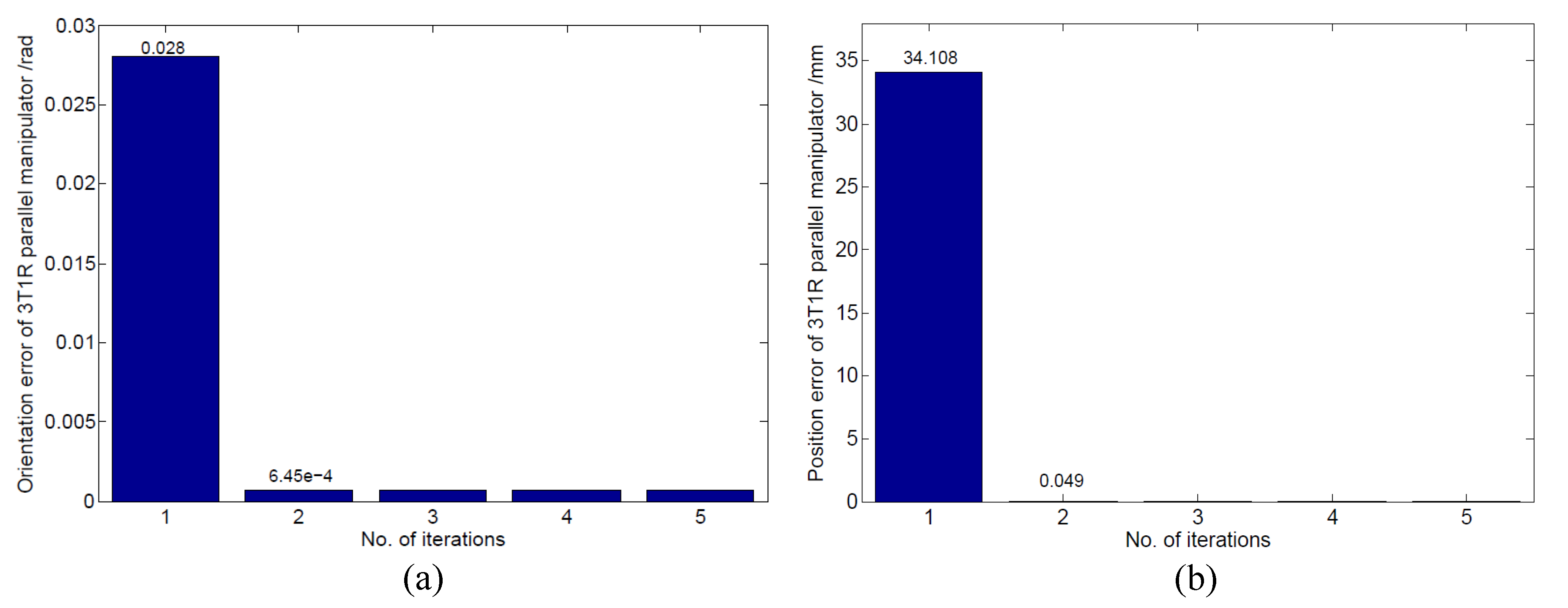
6. Simulation Results

The kinematic modeling schematic diagram and the establishment of the coordinate system are shown in Figure 3, where $l_u=0.7$, $l_d=0.7$, $a=0.3$, $b=1.0$ (units: m). According to the modeling method using the local POE formula given in Nomenclature, the values of the initial pose and joint twist of adjacent links of two branched chains are given as:

$T_{B,11}\left(0\right)=\left[\begin{array}{cccc}1\hfill & 0\hfill & 0\hfill & 0\hfill \\ 0\hfill & 1\hfill & 0\hfill & 0.03\hfill \\ 0\hfill & 0\hfill & 1\hfill & 0\hfill \\ 0\hfill & 0\hfill & 0\hfill & 1\hfill \end{array}\right]$, $T_{11,12}\left(0\right)=\left[\begin{array}{cccc}1\hfill & 0\hfill & 0\hfill & 0\hfill \\ 0\hfill & 1\hfill & 0\hfill & 0\hfill \\ 0\hfill & 0\hfill & 1\hfill & 0\hfill \\ 0\hfill & 0\hfill & 0\hfill & 1\hfill \end{array}\right]$,

$T_{12,13}\left(0\right)=\left[\begin{array}{cccc}1\hfill & 0\hfill & 0\hfill & 0\hfill \\ 0\hfill & cos\left(-\alpha \right)\hfill & -sin\left(-\alpha \right)\hfill & l_u\hfill \\ 0\hfill & sin\left(-\alpha \right)\hfill & cos\left(-\alpha \right)\hfill & 0\hfill \\ 0\hfill & 0\hfill & 0\hfill & 1\hfill \end{array}\right]$, $T_{13,14}\left(0\right)=\left[\begin{array}{cccc}cos(-\beta )\hfill & 0\hfill & sin(-\beta )\hfill & l_d\hfill \\ 0\hfill & 1\hfill & 0\hfill & 0\hfill \\ -sin(-\beta )\hfill & 0\hfill & cos\left(-\beta \right)\hfill & 0\hfill \\ 0\hfill & 0\hfill & 0\hfill & 1\hfill \end{array}\right]$,

$T_{14,P}\left(0\right)=\left[\begin{array}{cccc}1\hfill & 0\hfill & 0\hfill & a/2\hfill \\ 0\hfill & 1\hfill & 0\hfill & 0\hfill \\ 0\hfill & 0\hfill & 1\hfill & 0\hfill \\ 0\hfill & 0\hfill & 0\hfill & 1\hfill \end{array}\right]$, $T_{B,21}\left(0\right)=\left[\begin{array}{cccc}1\hfill & 0\hfill & 0\hfill & b\hfill \\ 0\hfill & 1\hfill & 0\hfill & 0.03\hfill \\ 0\hfill & 0\hfill & 1\hfill & 0\hfill \\ 0\hfill & 0\hfill & 0\hfill & 1\hfill \end{array}\right]$, $T_{21,22}\left(0\right)=\left[\begin{array}{cccc}1\hfill & 0\hfill & 0\hfill & 0\hfill \\ 0\hfill & 1\hfill & 0\hfill & 0\hfill \\ 0\hfill & 0\hfill & 1\hfill & 0\hfill \\ 0\hfill & 0\hfill & 0\hfill & 1\hfill \end{array}\right]$,

$T_{22,23}\left(0\right)=\left[\begin{array}{cccc}1\hfill & 0\hfill & 0\hfill & 0\hfill \\ 0\hfill & cos\left(-\alpha \right)\hfill & -sin\left(-\alpha \right)\hfill & l_u\hfill \\ 0\hfill & sin\left(-\alpha \right)\hfill & cos\left(-\alpha \right)\hfill & 0\hfill \\ 0\hfill & 0\hfill & 0\hfill & 1\hfill \end{array}\right]$, $T_{23,24}\left(0\right)=\left[\begin{array}{cccc}-cos\left(\beta \right)\hfill & 0\hfill & -sin\left(\beta \right)\hfill & l_d\hfill \\ 0\hfill & 1\hfill & 0\hfill & 0\hfill \\ sin\left(\beta \right)\hfill & 0\hfill & -cos\left(\beta \right)\hfill & 0\hfill \\ 0\hfill & 0\hfill & 0\hfill & 1\hfill \end{array}\right]$,

$T_{24,P}\left(0\right)=\left[\begin{array}{cccc}1\hfill & 0\hfill & 0\hfill & -a/2\hfill \\ 0\hfill & 1\hfill & 0\hfill & 0\hfill \\ 0\hfill & 0\hfill & 1\hfill & 0\hfill \\ 0\hfill & 0\hfill & 0\hfill & 1\hfill \end{array}\right]$,

$$s_{11}={\left[\begin{array}{cccccc}0\hfill & 1\hfill & 0\hfill & 0\hfill & 0\hfill & 0\hfill \end{array}\right]}^T,s_{12}={\left[\begin{array}{cccccc}0\hfill & 0\hfill & 0\hfill & 1\hfill & 0\hfill & 0\hfill \end{array}\right]}^T,$$

$$s_{13}={\left[\begin{array}{cccccc}0\hfill & 0\hfill & 0\hfill & 0\hfill & 1\hfill & 0\hfill \end{array}\right]}^T,s_{14}={\left[\begin{array}{cccccc}0\hfill & 0\hfill & 0\hfill & 0\hfill & 0\hfill & 1\hfill \end{array}\right]}^T,$$

$$s_{21}={\left[\begin{array}{cccccc}0\hfill & 1\hfill & 0\hfill & 0\hfill & 0\hfill & 0\hfill \end{array}\right]}^T,s_{22}={\left[\begin{array}{cccccc}0\hfill & 0\hfill & 0\hfill & 1\hfill & 0\hfill & 0\hfill \end{array}\right]}^T,$$

$$s_{23}={\left[\begin{array}{cccccc}0\hfill & 0\hfill & 0\hfill & 0\hfill & 1\hfill & 0\hfill \end{array}\right]}^T,s_{24}={\left[\begin{array}{cccccc}0\hfill & 0\hfill & 0\hfill & 0\hfill & 0\hfill & 1\hfill \end{array}\right]}^T.$$

In order to simulate the deviation of kinematic parameters from the nominal ones, the errors $\delta t$, $\delta s$, and $\delta q$ are applied to the initial poses, joint twists, and joint variables in the theoretical model. Noise is introduced in the measurement of joint variables to test the robustness of the parameter identification method. In this way, an actual model is obtained, where the actual initial pose is:

$$\begin{array}{c}\hfill T_{i(j-1),ij}^a\left(0\right)=e^{{\widehat{t}}_{ij}}{e}^{\delta {\widehat{t}}_{ij}}=T_{i(j-1),ij}\left(0\right)e^{\delta {\widehat{t}}_{ij}},\end{array}$$

(34)

the actual joint twist is:

$$\begin{array}{c}\hfill s_{ij}^a=s_{ij}+\delta s_{ij},\end{array}$$

(35)

the actual joint variable is:

$$\begin{array}{c}\hfill q_{ij}^a=q_{ij}+\delta q_{ij}.\end{array}$$

(36)

Hence, the kinematic model of the actual branched chain i is:

$$\begin{array}{c}\hfill g_i=T_{B,i1}^a\left(0\right)e^{{\widehat{s}}_{i1}^a{q}_{i1}^a}·T_{i1,i2}^a\left(0\right)e^{{\widehat{s}}_{i2}^a{q}_{i2}^a}·T_{i2,i3}^a\left(0\right)e^{{\widehat{s}}_{i3}^a{q}_{i3}^a}·T_{i3,i4}^a\left(0\right)e^{{\widehat{s}}_{i4}^a{q}_{i4}^a}·T_{i4,P}^a\left(0\right).\end{array}$$

(37)

Add deviations $\delta t$, $\delta s$, and $\delta q$ to the nominal values to get the actual value of the parallel manipulator simulation, as shown in

Table 1. Preset error of each link (all units are in SI).

$\mathit{Dyad}$	$\mathit{\delta }\mathit{t}$	$\mathit{\delta }\mathit{s}$	$\mathit{\delta }\mathit{q}$
B-11	${\left[\begin{array}{cccccc}0.002\hfill & 0.002\hfill & 0.002\hfill & 0.001\hfill & 0.001\hfill & 0.001\hfill \end{array}\right]}^T$	${\left[\begin{array}{cccccc}0\hfill & 0\hfill & 0\hfill & 0\hfill & 0\hfill & 0\hfill \end{array}\right]}^T$	0.02
11-12	${\left[\begin{array}{cccccc}0.002\hfill & 0.002\hfill & 0.002\hfill & 0.001\hfill & 0.001\hfill & 0.001\hfill \end{array}\right]}^T$	${\left[\begin{array}{cccccc}0\hfill & 0\hfill & 0\hfill & -1+cos0.02\hfill & sin0.02\hfill & 0\hfill \end{array}\right]}^T$	0.02
12-13	${\left[\begin{array}{cccccc}0.002\hfill & 0.002\hfill & 0.002\hfill & 0.001\hfill & 0.001\hfill & 0.001\hfill \end{array}\right]}^T$	${\left[\begin{array}{cccccc}0\hfill & 0\hfill & 0\hfill & 0\hfill & -1+cos0.02\hfill & sin0.02\hfill \end{array}\right]}^T$	0.02
13-14	${\left[\begin{array}{cccccc}0.002\hfill & 0.002\hfill & 0.002\hfill & 0.001\hfill & 0.001\hfill & 0.001\hfill \end{array}\right]}^T$	${\left[\begin{array}{cccccc}0\hfill & 0\hfill & 0\hfill & 0\hfill & sin0.02\hfill & -1+cos0.02\hfill \end{array}\right]}^T$	0.02
14-P	${\left[\begin{array}{cccccc}0.002\hfill & 0.002\hfill & 0.002\hfill & 0.001\hfill & 0.001\hfill & 0.001\hfill \end{array}\right]}^T$	\	\
B-21	${\left[\begin{array}{cccccc}0.002\hfill & 0.002\hfill & 0.002\hfill & 0.001\hfill & 0.001\hfill & 0.001\hfill \end{array}\right]}^T$	${\left[\begin{array}{cccccc}0\hfill & 0\hfill & 0\hfill & 0\hfill & 0\hfill & 0\hfill \end{array}\right]}^T$	0.02
21-22	${\left[\begin{array}{cccccc}0.002\hfill & 0.002\hfill & 0.002\hfill & 0.001\hfill & 0.001\hfill & 0.001\hfill \end{array}\right]}^T$	${\left[\begin{array}{cccccc}0\hfill & 0\hfill & 0\hfill & 1-cos0.02\hfill & sin0.02\hfill & 0\hfill \end{array}\right]}^T$	0.02
22-23	${\left[\begin{array}{cccccc}0.002\hfill & 0.002\hfill & 0.002\hfill & 0.001\hfill & 0.001\hfill & 0.001\hfill \end{array}\right]}^T$	${\left[\begin{array}{cccccc}0\hfill & 0\hfill & 0\hfill & 0\hfill & -1+cos0.02\hfill & sin0.02\hfill \end{array}\right]}^T$	0.02
23-24	${\left[\begin{array}{cccccc}0.002\hfill & 0.002\hfill & 0.002\hfill & 0.001\hfill & 0.001\hfill & 0.001\hfill \end{array}\right]}^T$	${\left[\begin{array}{cccccc}0\hfill & 0\hfill & 0\hfill & 0\hfill & sin0.02\hfill & -1+cos0.02\hfill \end{array}\right]}^T$	0.02
24-P	${\left[\begin{array}{cccccc}0.002\hfill & 0.002\hfill & 0.002\hfill & 0.001\hfill & 0.001\hfill & 0.001\hfill \end{array}\right]}^T$	\	\

. Each joint, regardless of being active or passive, is considered as a joint with one degree of freedom, so the error vector of the spin volume should be orthonormal, that is $∥w_i+\delta w∥=1$,${\left(w_i+\delta w\right)}^T\left(v_i+\delta v\right)=0$.

Now, the simulation process of the kinematic error modeling and parameter identification is summarized as follows:

1.

Use the numerical forward kinematics algorithm to obtain the joint displacements and joint angles of 20 different parallel manipulator poses;

2.

Assign errors to kinematic parameters, such as $\delta t$, $\delta s$, and $\delta q$, as shown in Table 1.

3.

Simulate the actual initial pose using $T_{i(j-1),ij}^a\left(0\right)=T_{i(j-1),ij}\left(0\right)e^{\delta {\widehat{t}}_{ij}}$;

4.

The actual joint twist is computed as $s_{ij}^a=s_{ij}+\delta s_{ij}$;

5.

The actual joint variable is computed as $q_{ij}^a=q_{ij}+\delta q_{ij}$;

6.

The recursive calibration algorithm is used to identify the kinematic errors of the parallel manipulator.

The initial pose after calibration is recorded as $T_{i(j-1),ij}^c\left(0\right)$, as shown in

Table 2. Kinematic error of each link versus its calibration pose (all units are in SI).

$\mathit{Dyad}$	Kinematic Errors	${\mathit{T}}_{\mathit{i}(\mathit{j}-1),\mathit{ij}}^{\mathit{c}}\left(0\right)$
$B-11$	${(1.824,2.272,1.183,0.02000,0.00128,0.00100)}^T$	$\left[\begin{array}{cccc}1.00000\hfill & -0.00099\hfill & 0.00129\hfill & 1.794\hfill \\ 0.00102\hfill & 0.99980\hfill & -0.02000\hfill & 32.255\hfill \\ -0.00127\hfill & 0.02000\hfill & 0.99980\hfill & 1.805\hfill \\ 0\hfill & 0\hfill & 0\hfill & 1\hfill \end{array}\right]$
$11-12$	${(1.794,2.272,1.783,0.02000,0.00128,0.00165)}^T$	$\left[\begin{array}{cccc}1.00000\hfill & -0.00164\hfill & 0.00128\hfill & 1.793\hfill \\ 0.00165\hfill & 0.99999\hfill & -0.00201\hfill & 2.272\hfill \\ -0.00128\hfill & 0.00201\hfill & 1.00000\hfill & 1.784\hfill \\ 0\hfill & 0\hfill & 0\hfill & 1\hfill \end{array}\right]$
$12-13$	${(2.855,2.868,-1.922,0.00225,0.00207,0.00152)}^T$	$\left[\begin{array}{cccc}1.00000\hfill & -0.00253\hfill & 0.00039\hfill & 1.791\hfill \\ 0.00152\hfill & 0.70869\hfill & 0.70551\hfill & 702.869\hfill \\ -0.00207\hfill & -0.70551\hfill & 0.70870\hfill & 0.344\hfill \\ 0\hfill & 0\hfill & 0\hfill & 1\hfill \end{array}\right]$
$13-14$	${(-0.647,1.134,3.916,-0.00107,0.00210,0.00163)}^T$	$\left[\begin{array}{cccc}0.50182\hfill & -0.00163\hfill & -0.86497\hfill & 699.353\hfill \\ 0.00174\hfill & 1.00000\hfill & -0.00087\hfill & 2.273\hfill \\ 0.86497\hfill & -0.00107\hfill & 0.50182\hfill & 2.445\hfill \\ 0\hfill & 0\hfill & 0\hfill & 1\hfill \end{array}\right]$
$14-P$	${(1.794,2.063,2.139,0.000874,0.00237,0.00140)}^T$	$\left[\begin{array}{cccc}1.00000\hfill & -0.00140\hfill & 0.00237\hfill & 151.795\hfill \\ 0.00140\hfill & 1.00000\hfill & -0.00087\hfill & 2.273\hfill \\ -0.00237\hfill & 0.00088\hfill & 1.00000\hfill & 1.782\hfill \\ 0\hfill & 0\hfill & 0\hfill & 1\hfill \end{array}\right]$
$B-21$	${(1.790,2.153,2.123,0.02000,0.00175,0.00100)}^T$	$\left[\begin{array}{cccc}0.99999\hfill & -0.00099\hfill & 0.00176\hfill & 1001.760\hfill \\ 0.00102\hfill & 0.99980\hfill & -0.02000\hfill & 33.147\hfill \\ -0.00174\hfill & 0.02000\hfill & 0.99980\hfill & 1.007\hfill \\ 0\hfill & 0\hfill & 0\hfill & 1\hfill \end{array}\right]$
$21-22$	${(1.761,3.155,0.977,0.00165,0.00175,0.00050)}^T$	$\left[\begin{array}{cccc}1.00000\hfill & -0.00050\hfill & 0.00175\hfill & 1.761\hfill \\ 0.00051\hfill & 1.00000\hfill & -0.00165\hfill & 3.155\hfill \\ -0.00174\hfill & 0.00165\hfill & 1.00000\hfill & 0.978\hfill \\ 0\hfill & 0\hfill & 0\hfill & 1\hfill \end{array}\right]$
$22-23$	${(2.009,2.922,-0.003,0.00273,0.00159,0.00035)}^T$	$\left[\begin{array}{cccc}1.00000\hfill & -0.00137\hfill & 0.00088\hfill & 1.759\hfill \\ 0.00036\hfill & 0.70903\hfill & 0.70518\hfill & 702.924\hfill \\ -0.00159\hfill & -0.70517\hfill & 0.70903\hfill & -0.00154\hfill \\ 0\hfill & 0\hfill & 0\hfill & 1\hfill \end{array}\right]$
$23-24$	${(-1.726,3.529,2.156,-0.00256,0.00160,-0.00053)}^T$	$\left[\begin{array}{cccc}-0.49861\hfill & 0.00053\hfill & -0.86682\hfill & 698.275\hfill \\ 0.00248\hfill & 1.00000\hfill & -0.00081\hfill & 3.157\hfill \\ 0.86682\hfill & -0.00256\hfill & -0.49861\hfill & 1.034\hfill \\ 0\hfill & 0\hfill & 0\hfill & 1\hfill \end{array}\right]$
$24-P$	${(1.761,3.598,0.759,0.00082,0.00145,0.00295)}^T$	$\left[\begin{array}{cccc}1.00000\hfill & -0.00295\hfill & 0.00145\hfill & -148.243\hfill \\ 0.00295\hfill & 1.00000\hfill & -0.00081\hfill & 3.157\hfill \\ -0.00145\hfill & 0.00082\hfill & 1.00000\hfill & 0.977\hfill \\ 0\hfill & 0\hfill & 0\hfill & 1\hfill \end{array}\right]$

. When $\mathrm{trace}\left(R\right)\ne -1$, $1+2cos\varphi =\mathrm{trace}\left(R\right)$, and $\parallel \omega \parallel <\pi$, we get $log\left(T\right)=t$. That is,

$$\begin{array}{c}\hfill log\left[\begin{array}{cc}R\hfill & p\hfill \\ 0\hfill & 1\hfill \end{array}\right]=\left[\begin{array}{cc}\widehat{\omega }\hfill & A^{*}p\hfill \\ 0\hfill & 0\hfill \end{array}\right]\in se\left(3\right),\end{array}$$

(38)

where,

$$\widehat{\omega }=logR=\frac{\varphi }{2sin\varphi }(R-R^T),$$

$$A^{*}=I-\frac{1}{2}\widehat{\omega }+\frac{2sin\parallel \omega \parallel -\parallel \omega \parallel (1+cos\parallel \omega \parallel )}{2{\parallel \omega \parallel }^{2}sin\parallel \omega \parallel }{\widehat{\omega }}^2,$$

If $\varphi$ is small, $\widehat{\omega }\approx (R-R^T)/2$. When $\mathrm{trace}\left(R\right)=-1$, $logR=(2k+1)\pi \widehat{\nu }$. In this case, k is any integer, and $\nu$ is a unit eigenvector of $logR$ with an eigenvalue of one.

The kinematic error between the calibrated value $T^c$ and the actual value $T^a$ is obtained through the above method, as shown in Table 2, including the orientation and position error at the end effector. The orientation error is the angular difference between the actual value of the end effector and the calibrated one. Position error is the norm of the coordinate difference between the actual value of the midpoint of the moving platform and the calibration one. Note that the derivation of kinematic parameters was arbitrarily assumed in this simulation example, and it may not truly reflect the actual situation in the parameter space due to manufacturing and assembly error. However, through the end effector’s pose error simulation result as in Figure 4, it is seen that both the orientation and position errors converged, and they were reduced by at least 10 times, thereby verifying the effectiveness of the calibration algorithm. Compared with other methods based on the deviation of the distance between points on the end-effector of parallel manipulators [26,27], our method gave better fitness of the pose error at the central point of the end effector. Since the model was linear-in-parameter, the pose fit with higher matching and better fitting conversion effects. Therefore, in the case of a linear error model, the pose error was used for fitting so that the error reduction only needed one iteration.

To guide the future calibration experiments, the flowchart of the calibration process is given in Figure 5. The meanings of various symbols in the flowchart can be referenced in Nomenclature.

7. Pre-Processing Compensation

Since some robot controllers cannot directly utilize the calibrated active and passive joint angles to drive the robot, the joint variables were preprocessed to obtain the pose of the end effector that could be directly utilized by the robot.

First, the initial pose $T_{i(j-1),ij}^c\left(0\right)$ after calibration of each link was obtained through the calibration process described above, as shown in Table 2. Combined with the commanded end pose $T_{co}$, the calibrated joint angle $q_{ij}^c$ was calculated using the inverse kinematics after calibration. Since the manipulator could not directly use $q_{ij}^c$, the following conversion was required. By bringing $q_{ij}^c$ into the positive kinematics solution based on the nominal kinematics parameters, the compensated end effector pose $T_{cp}$ could be obtained. At this time, $T_{cp}$ could be directly used for offline programming. The flowchart of this process is shown in Figure 6. The meaning of various symbols is listed in Nomenclature.

8. Conclusions

In this paper, a kinematic model of a symmetrical 3T1R parallel manipulator was proposed based on the local POE formula. By using local POE formula for kinematic error modeling, the joint twists and joint variables could maintain their nominal values, and the errors were set to be concentrated in the matrices of initial poses. As the end effector’s pose errors of the parallel manipulator established through different branched chains were identical, the entire pose error of the parallel manipulator’s end effector was formed by equaling the pose error of the end effector calculated in individual branched chains.In addition, the joint angle of the second revolute joint was calculated by a recursive algorithm according to the inherent kinematic constraints. This saved the rotary sensors installed at the second revolute joint of each branched chain. Through simulation, it was shown that the deviation between the actual and calibrated end effector’s pose could be reduced by at least 10 times with the proposed kinematic error modeling and parameter identification methods. The procedures to use this error model for profile pre-compensation in the actual testbed were also proposed.

References

1. Stewart, D. A platform with six degrees of freedom. Proc. Inst. Mech. Eng. 1965, 180, 371–386. [Google Scholar] [CrossRef]
2. Wu, C.; Yang, G.; Chen, C.; Liu, S.; Zheng, T. Kinematic design of a novel 4-dof parallel manipulator. In Proceedings of the 2017 IEEE International Conference on Robotics and Automation (ICRA), Singapore, 29 May–3 June 2017; pp. 6099–6104. [Google Scholar]
3. Wu, J.-F.; Zhang, R.; Wang, R.-H.; Yao, Y.-X. A systematic optimization approach for the calibration of parallel kinematics machine tools by a laser tracker. Int. J. Mach. Tools Manuf. 2014, 86, 1–11. [Google Scholar] [CrossRef]
4. Chanal, H.; Duc, E.; Ray, P.; Hascoet, J.Y. A new approach for the geometrical calibration of parallel kinematics machines tools based on the machining of a dedicated part. Int. J. Mach. Tools Manuf. 2007, 47, 1151–1163. [Google Scholar] [CrossRef]
5. Fu, J.; Gao, F.; Chen, W.; Pan, Y.; Lin, R. Kinematic accuracy research of a novel six-degree-of-freedom parallel robot with three legs. Mech. Mach. Theory 2016, 102, 86–102. [Google Scholar] [CrossRef]
6. Song, Y.; Zhang, J.; Lian, B.; Sun, T. Kinematic calibration of a 5-dof parallel kinematic machine. Precis. Eng. 2016, 45, 242–261. [Google Scholar] [CrossRef]
7. Sun, T.; Zhai, Y.; Song, Y.; Zhang, J. Kinematic calibration of a 3-dof rotational parallel manipulator using laser tracker. Robot. -Comput.-Integr. Manuf. 2016, 41, 78–91. [Google Scholar] [CrossRef]
8. Liu, H.; Gong, M.; O, M.Z.H.A. Error analysis and calibration of a 4-dof parallel mechanism. Robot 2005, 27, 6–9. [Google Scholar]
9. Hartenberg, R.S.; Denavit, J. A kinematic notation for lower pair mechanisms based on matrices. J. Appl. Mech. 1955, 77, 215–221. [Google Scholar]
10. Mooring, B.W. An improved method for identifying the kinematic parameters in a six axes robots. In Computers in Engineering, Proceedings of the International Computers in Engineering Conference and Exhibit; American Soc of Mechanical Engineers (ASME): New York, NY, USA, 1984; Volume 1, pp. 79–84. [Google Scholar]
11. Yang, G.; Chen, I.-M.; Lee, W.K.; Yeo, S.H. Self-calibration of three-legged modular reconfigurable parallel robots based on leg-end distance errors. Robotica 2001, 19, 187–198. [Google Scholar] [CrossRef]
12. Chen, G.; Kong, L.; Li, Q.; Wang, H.; Lin, Z. Complete, minimal and continuous error models for the kinematic calibration of parallel manipulators based on poe formula. Mech. Mach. Theory 2018, 121, 844–856. [Google Scholar] [CrossRef]
13. Okamura, K.; Park, F.C. Kinematic calibration using the product of exponentials formula. Robotica 1996, 14, 415–421. [Google Scholar] [CrossRef]
14. He, R.; Zhao, Y.; Yang, S.; Yang, S. Kinematic-parameter identification for serial-robot calibration based on poe formula. IEEE Trans. Robot. 2010, 26, 411–423. [Google Scholar]
15. Wang, H.; Shen, S.; Lu, X. A screw axis identification method for serial robot calibration based on the poe model. Ind. Robot. Int. J. 2012, 39, 146–153. [Google Scholar] [CrossRef] [Green Version]
16. Chen, I.-M.; Yang, G.; Tan, C.T.; Yeo, S.H. Local poe model for robot kinematic calibration. Mech. Mach. Theory 2001, 36, 1215–1239. [Google Scholar] [CrossRef]
17. Nubiola, A.; Bonev, I.A. Absolute robot calibration with a single telescoping ballbar. PRecision Eng. 2014, 38, 472–480. [Google Scholar] [CrossRef]
18. Joubair, A.; Slamani, M.; Bonev, I.A. Kinematic calibration of a five-bar planar parallel robot using all working modes. Robot. -Comput.-Integr. Manuf. 2013, 29, 15–25. [Google Scholar] [CrossRef]
19. Du, G.; Zhang, P. Online robot calibration based on vision measurement. Robot. Comput.-Integr. Manuf. 2013, 29, 484–492. [Google Scholar] [CrossRef]
20. HuangFu, Y.; Hang, L.; Cheng, W.; Yu, L.; Shen, C.; Wang, J.; Qin, W.; Wang, Y. Research on robot calibration based on laser tracker. In Mechanism and Machine Science; Springer: Berlin/Heidelberg, Germany, 2016; pp. 1475–1488. [Google Scholar]
21. Elatta, A.Y.; Gen, L.P.; Zhi, F.L.; Daoyuan, Y.; Fei, L. An overview of robot calibration. Inf. Technol. J. 2004, 3, 74–78. [Google Scholar]
22. Wu, L.; Yang, X.; Chen, K.; Ren, H. A minimal poe-based model for robotic kinematic calibration with only position measurements. IEEE Trans. Autom. Sci. Eng. 2014, 12, 758–763. [Google Scholar] [CrossRef]
23. Sareh, P. The least symmetric crystallographic derivative of the developable double corrugation surface: Computational design using underlying conic and cubic curves. Mater. Des. 2019, 183, 108128. [Google Scholar] [CrossRef]
24. Chen, J.; San, H.; Wu, X.; Chen, M.; He, W. Structural design and characteristic analysis for a 4-degree-of-freedom parallel manipulator. Adv. Mech. Eng. 2019, 11, 1687814019850995. [Google Scholar] [CrossRef]
25. Yang, L.; Tian, X.; Li, Z.; Chai, F.; Dong, D. Numerical simulation of calibration algorithm based on inverse kinematics of the parallel mechanism. Optik 2019, 182, 555–564. [Google Scholar] [CrossRef]
26. Huang, K.; Liu, R.G.; Wu, J.S.; Lao, X.R.; Mo, J.H. Parameter calibration method based on screw theory for articulated coordinate measuring arm. In Advanced Materials Research; Trans Tech Publ: Zurich, Switzerland, 2011; Volume 189, pp. 4049–4052. [Google Scholar]
27. Gu, L.; Yang, G.; Fang, Z.; Shen, W.; Zheng, T.; Chen, C.; Zhang, C. A two-step self-calibration method with portable measurement devices for industrial robots based on poe formula. In International Conference on Intelligent Robotics and Applications; Springer: Berlin/Heidelberg, Germany, 2019; pp. 715–727. [Google Scholar]
Figure 1. Basic structure figure of this 3T1R parallel manipulator.
Symmetry 12 00357 g001
Figure 2. D y a d kinematics based on different methods of establishing coordinate systems for the local POE formula. (a) to establish a coordinate system arbitrarily, (b) to establish a coordinate system which leads to reduced number of kinematic parameters.
Symmetry 12 00357 g002
Figure 3. Mechanism schematic of this 3T1R parallel manipulator. (a) the schematic of the 3T1R parallel manipulator; (b) the establishment of the coordinate system.
Symmetry 12 00357 g003
Figure 4. The end effector’s pose error simulation result. (a) Orientation error; (b) position error.
Symmetry 12 00357 g004
Figure 5. Flowchart of the calibration.
Symmetry 12 00357 g005
Figure 6. Flowchart of pre-processing compensation.
Symmetry 12 00357 g006