Article

Fractional Dynamics in Soccer Leagues

by
António M. Lopes
1,* and
Jose A. Tenreiro Machado
2
1
UISPA–LAETA/INEGI, Faculty of Engineering, University of Porto, Rua Dr. Roberto Frias, 4200-465 Porto, Portugal
2
Institute of Engineering, Polytechnic of Porto, Department of Electrical Engineering, Rua Dr. António Bernardino de Almeida, 431, 4249-015 Porto, Portugal
*
Author to whom correspondence should be addressed.
Symmetry 2020, 12(3), 356; https://doi.org/10.3390/sym12030356
Submission received: 27 January 2020 / Revised: 14 February 2020 / Accepted: 16 February 2020 / Published: 1 March 2020
(This article belongs to the Special Issue Bifurcation and Chaos in Fractional-Order Systems)

Abstract

:
This paper addresses the dynamics of four European soccer teams over the season 2018–2019. The modeling perspective adopts the concepts of fractional calculus and power law. The proposed model embeds implicitly details such as the behavior of players and coaches, strategical and tactical maneuvers during the matches, errors of referees and a multitude of other effects. The scale of observation focuses the teams’ behavior at each round. Two approaches are considered, namely the evaluation of the team progress along the league by a variety of heuristic models fitting real-world data, and the analysis of statistical information by means of entropy. The best models are also adopted for predicting the future results and their performance compared with the real outcome. The computational and mathematical modeling lead to results that are analyzed and interpreted in the light of fractional dynamics. The emergence of patterns both with the heuristic modeling and the entropy analysis highlight similarities in different national leagues and point towards some underlying complex dynamics.

1. Introduction

Soccer is the most popular sport in Europe [1,2]. The game is played by two teams of 11 players, on a rectangular field with a goal placed at each end. The objective of the game is to score by getting a spherical ball into the opposing goal. Each team includes 10 field players, that can maneuver the ball using any part of the body except hands and arms, and one goalkeeper, who is allowed to touch the ball with the whole body, as long as they stay in their penalty area. Otherwise, the rules of the field players apply. The match has two periods of 45 minutes each. The winning team is the one that scores more goals by the end of the match.
In most European countries, soccer competitions are organized hierarchically in leagues composed by groups of teams. At the end of each season, a promotion and relegation system decides which teams move up and down into the hierarchy. In a given league and season each pair of teams plays to matches, so that the visited and visitor interchange place. All teams start with zero points and, at every round, one {victory, draw, defeat} is worth { 3 , 1 , 0 } points. By the end of the last round, the team that accumulated more points is the champion [3].
This paper studies the dynamical performance of soccer teams in a given league. The modeling perspective adopts the concepts of fractional calculus [4,5] and power law (PL) [6]. These tools have been used to model dynamical systems with memory in mechanics [7], electromagnetism [8], biology [9], sports [10], economy [11], and others [12]. The proposed approach embeds implicitly details such as the behavior of players and coaches, strategical and tactical maneuvers during the matches, errors of referees and a multitude of other effects. The scale of observation addresses the teams behavior in the perspective of their classification along the league. Data characterizing the year 2018–2019 and the four leagues, namely the Spanish ‘La Liga’, English ‘Premiership’, Italian ‘Serie A’ and French ‘Ligue 1’, are processed and discussed. The computational and mathematical modeling leads to the emergence of patterns that are analyzed and interpreted in the light of fractional dynamics.
In spite of its social and economical importance, the topic of soccer dynamics has been the subject of only a restricted number of studies. In fact, we can consider the study of the dynamic effects at different levels, namely about the evolution of each player along his career, of the evolution of the players within a given match, or the progress of the classification of a group of teams along a given league. Couceiro et al. [13] characterized the predictability and stability levels of players during a soccer match by means of fractional calculus and entropy measures. Silva et al. [14] investigated how different entropy measures can be applied to assess the performance variability and to uncover the interactions underlying the players and teams’ performance. Machado and Lopes [15] adopted distinct dissimilarity measures and multidimensional scaling to study the behavior of teams competing within soccer national leagues and related the generated loci with the teams’ performance over time. Neuman et al. [16] measured the organization associated with the behavior of a soccer team through the Tsallis entropy of ball passes between the players. They found that the teams’ positions at the end of one season were correlated with the teams entropy. Moreover, the entropy score could be used for predicting of the teams’ final positions. Lopes and Machado [17] studied the dynamics of national soccer leagues using information and fractional calculus tools. In their approach, an entire soccer league season was treated as a complex system with a state observable at the time of rounds, consisting of the goals scored by the teams. The system behavior was visualized in 3-D maps generated by multidimensional scaling and interpreted based on the emerging clusters.
Predicting the outcome of soccer matches has been investigated since at least the 1960s, due to its interests for the general public, clubs, advertising companies, media, professional odds setters, and researchers [18]. Various statistical techniques have been used, including Poisson models [19], Bayesian schemes [20], rating systems [21], and machine learning methods [22,23], such as kernel-based relational learning [24], among others [25,26]. Advanced machine learning techniques [27,28] may be of relevance and represent an alternative to statistical or analytical approaches. However, dynamical phenomena involving complex memory effects need to be analyzed under the light of modeling tools to better understand phenomena embedded in the data series. Therefore, a synergistic strategy encompassing studies of distinct nature seems the best to consider at the moment of writing this paper.
This paper addresses the dynamics exhibited by several leagues having in mind the evolution of the teams along one season. The adoption of heuristic models, fitting real-world data, and the entropy analysis of statistical information, give a new perspective to a complex system that has been scarcely studied in the scientific literature.
Bearing these ideas in mind, this paper is organized as follows. Section 2 models the behavior of the teams in four top European soccer leagues by means of different functions. Section 3 analyzes the leagues in the perspective of the entropy of the spatio-temporal patterns exhibited by distinct alternative models. Section 4 uses the models for predicting future results and assesses their accuracy. Finally, Section 5 outlines the conclusions.

2. Modeling the Teams’ Dynamics

Let us consider N teams competing in a league for one season. Therefore, the league has R = 2 ( N 1 ) rounds, and each team plays N 1 matches at home and N 1 matches away.
Let us denote by x i ( k ) , i = 1 , , N , 0 k k r , the teams’ positions from the beginning of the season up to the round k r = 3 , , R . The lower limit k r = 3 is adopted to yield data-series with a minimum number of points for processing. Therefore, the signals x i ( k ) evolve in discrete time and one-dimensional space, and can be seen as the output of a complex system.
We use the nonlinear least-squares [29,30] to test the behavior of the series x i ( k ) for six fitting hypotheses, namely shifted power (SP), quadratic (Qu), Hill (Hi), vapor pressure (VP), power law (PL) and Hoerl (Ho) models, given by:
S P : x ^ i S P ( k ) = a i ( k r ) · | k b i ( k r ) | c i ( k r ) ,
Q u : x ^ i Q u ( k ) = a i ( k r ) + b i ( k r ) · k + c i ( k r ) · k 2 ,
H i : x ^ i H i ( k ) = a i ( k r ) · k b i ( k r ) c i ( k r ) b i ( k r ) + k b i ( k r ) ,
V P : x ^ i V P ( k ) = e a i ( k r ) + b i ( k r ) c i ( k r ) · ln ( k ) ,
P L : x ^ i P L ( k ) = a i ( k r ) · k b i ( k r ) ,
H o : x ^ i H o ( k ) = a i ( k r ) · b i ( k r ) k · k c i ( k r ) ,
where x ^ i denotes the approximated values, k represents time and { a i ( k r ) , b i ( k r ) , c i ( k r ) } R are the models’ parameters. Naturally, for each model, the parameters vary with time, that is, they depend on k r .
We can adopt other fitting models, eventually with more parameters, that adjust better to some particular series x i ( k ) . However, only simple analytical expressions, requiring a limited set of parameters, are considered [31], otherwise the interpretation of the parameters becomes unclear. Moreover, loosely speaking, with exception of Qu, these heuristic models reflect somehow fractional characteristics, embodied in their structures by the non-integer exponents.
For assessing the accuracy of the models (1a)–(1f) we adopt the time varying errors E i and E given by:
E i ( k r ) = x i ( k r ) x ^ i ( k r ) , i = 1 , , N , k r = 3 , , R ,
E ( k r ) = 1 N i = 1 N [ E i ( k r ) ] 2 , k r = 3 , , R ,
where N = 20 and R = 38 correspond to the number of teams and rounds in the ‘La Liga’, ‘Premiership’, ‘Serie A’ and ‘Ligue 1’. Therefore, E i gives information for team i, while E highlights the fitting error for all teams involved in the league.
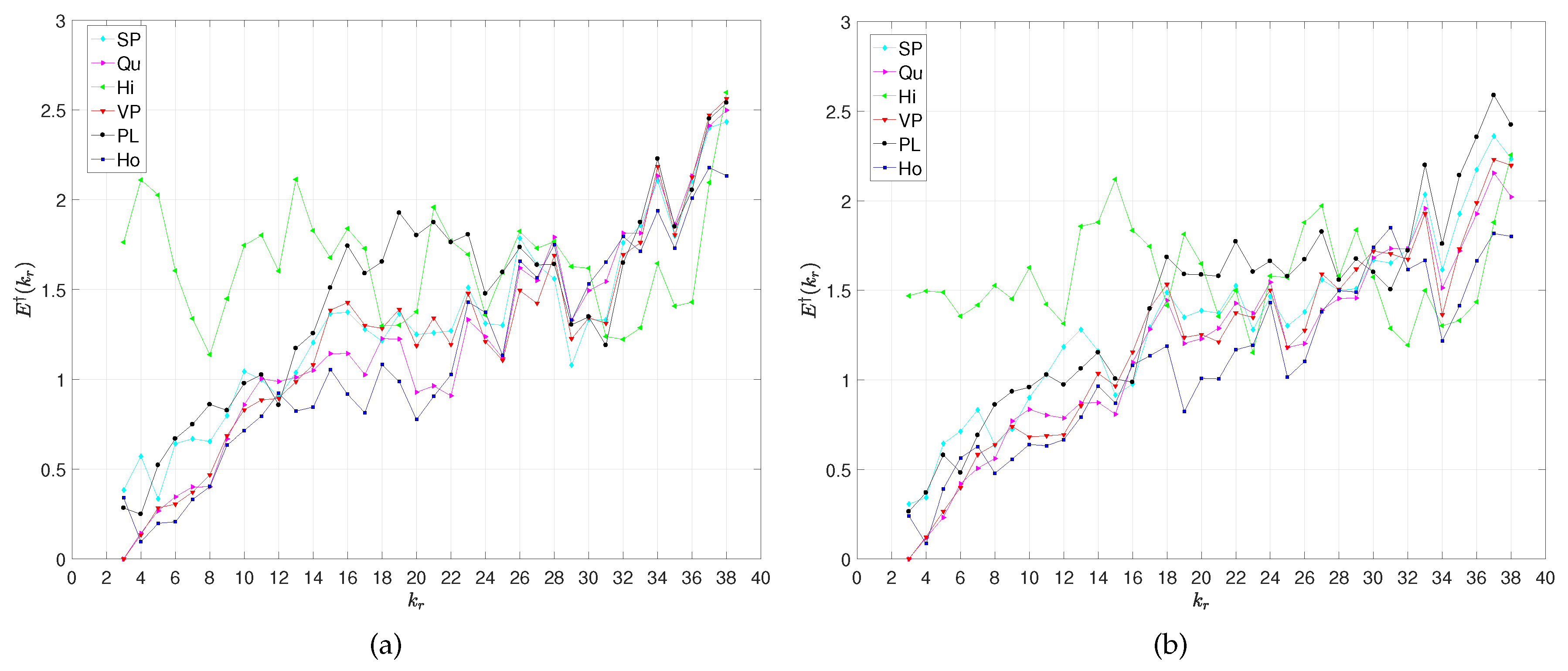
Figure 1 illustrates the error E 1 ( k r ) for the 2018–2019 champions of ‘La Liga’ and “Premiership”, namely the FC Barcelona and Manchester City, and the models (1a)–(1f). Figure 2 depicts E ( k r ) for ‘La Liga’ and ‘Premiership’. Obviously, this error increases with the number of data points. Moreover, we verify that, with the exception of the Hi (1c), all other models approximate well the data, demonstrating the adequacy of the fitting functions. The other teams and leagues yield charts of the same type and, therefore, are omitted herein. For a more assertive comparison, we calculate the mean and the standard deviation, μ = 1 36 k r = 3 38 E ( k r ) and σ = 1 36 k r = 3 38 [ E ( k r ) μ ] 2 , of the E ( k r ) series for the models (1a)–(1f). Table 1 summarizes the corresponding values, highlighting that the Ho (1f) is the best three-parameter model approximation, and that the PL (1e) represents a good alternative, when having in mind the advantage of having just two parameters.
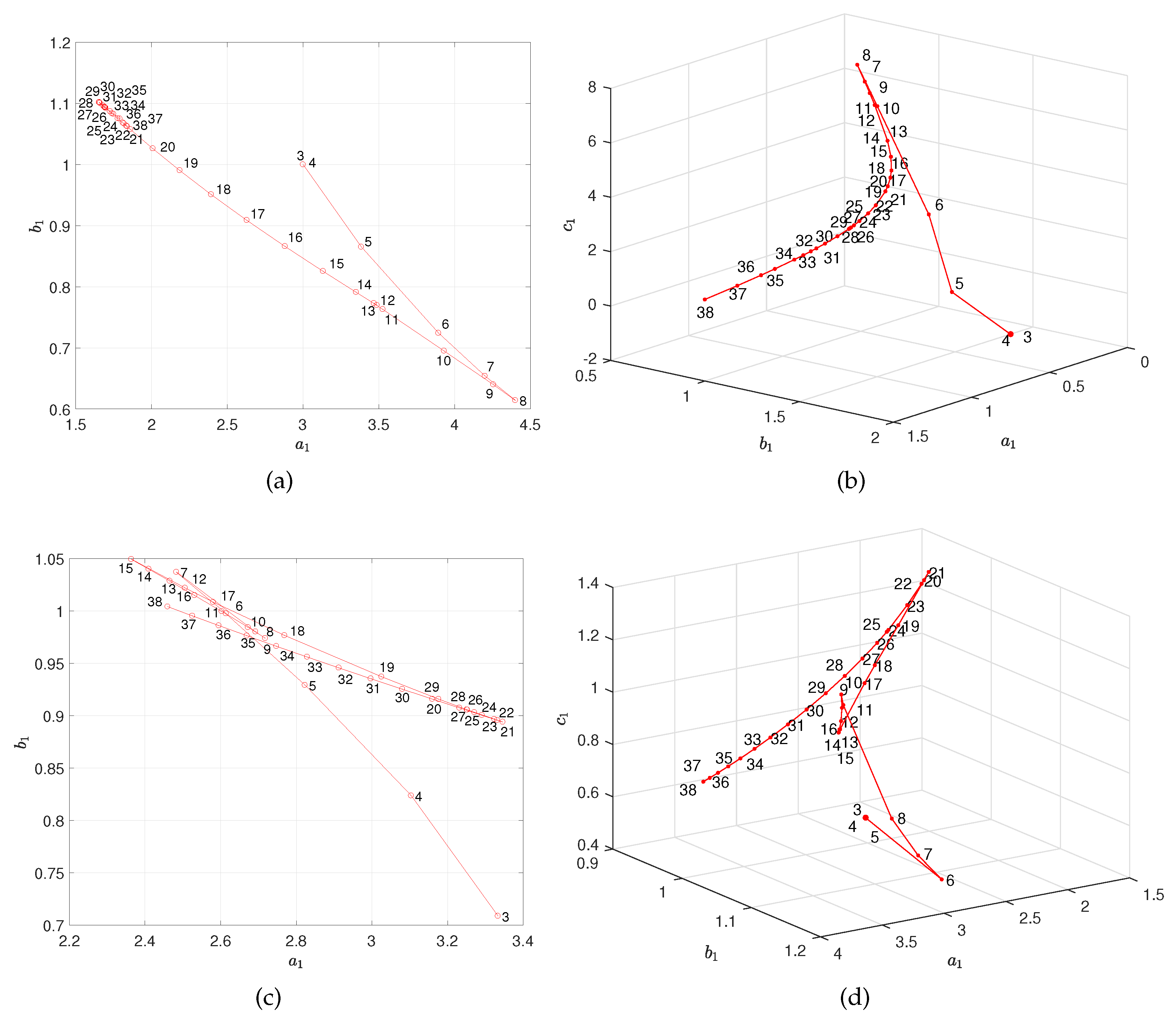
Figure 3 depicts the parameters { a 1 ( k r ) , b 1 ( k r ) } of the PL and { a 1 ( k r ) , b 1 ( k r ) , c 1 ( k r ) } for the Ho model for FC Barcelona and Manchester City, respectively. The point labels represent the value of k r . We verify that for the FC Barcelona we have two distinct periods in the locus. The first corresponds to 3 k r 8 , where the parameters evolve influenced by a set of consecutive bad results between rounds five and eight. The second period corresponds to 8 k r 38 , where the path changes direction driven by a consistent and positive team behavior towards the final victory at k r = 38 . For the Manchester City the variation of the parameters is more complex. Initially, we observe a route for the period 3 k r 7 . Then, the locus has a slight change, due to a draw achieved by the team at round 8, but recovers fast its initial trend during for 9 k r 15 . Again the locus changes driven by the set of team negative results in rounds 16–19 and 24. From k r = 25 onward, the parameters evolve positively influenced by the consecutive team victories until the end of the season at k r = 38 . For other teams we can draw similar conclusions, meaning that there exists a clear relationship between the models’ parameters and the teams’ performance along the season. Moreover, we verify that, in general, abrupt changes in the loci route correspond to inconsistent results at early rounds, that is, small values of k r . For larger values of k r , eventual inconsistencies on the teams’ behavior do not translate in significant modifications of the parameter patterns, since the fitting becomes less sensitive to the number of fitting points.

3. Entropy of the Spatio-Temporal Patterns of the Models’ Parameters

In this section we characterize the soccer leagues by means of entropy. The entropy is a measure of regularity that has been successfully adopted in the study of complex systems [15,32].

3.1. The Entropy of the PL Model

By approximating the output signals x i ( k ) through PL functions (1e) we are modeling the complex system as a fractional integrator [33,34] of order b i R + for a constant, step-like, input signal.
If a team obtains {victory, draw, defeat} in all matches, then x i ( k ) is a straight line with a i = { 3 , 1 , 0 } and b i = 1 . However, real-world teams have {victories, draws, defeats} and, thus, yield a fractal like response that follows a PL behavior. Therefore, fractional/unit values of b i reflect variable/constant time evolution, while values of a i close to { 3 , 1 , 0 } correspond to {victory, draw, defeat} results [10].
For each league we now compute the PL parameters { a i , b i } that fit the teams’ positions x i ( k ) , i = 1 , , 20 , 0 k k r , from the beginning of the season up to the round k r = 3 , , 38 . Therefore, for every k r we have an array of 20 × ( k r 2 ) points in a two-dimensional space. We then determine the bi-dimensional histograms by binning the data of each array into M × M = 100 × 100 bins { α j , β k } , j , k = 1 , , M . Finally, we calculate the Shannon entropy [35,36]:
S ( k r ) = j = 1 M k = 1 M P ( α j , β k ) log P ( α j , β k ) ,
where the probabilities P ( α j , β k ) are approximated by the data relative frequencies.
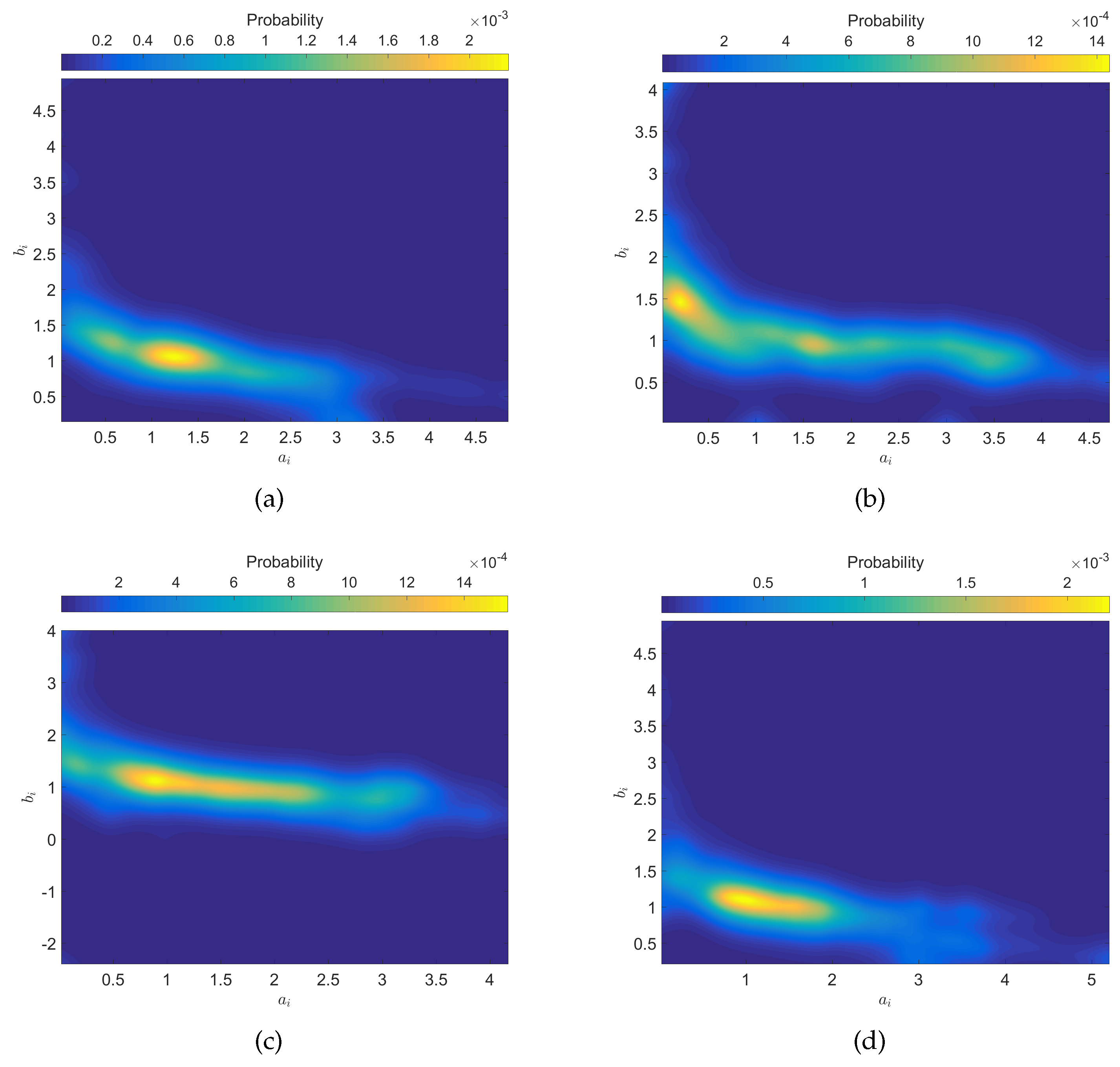
For example, Figure 4 depicts the histograms of the PL parameters from the beginning, k r = 3 , up to the end of the 2018–2019 season, k r = 38 , for ‘La Liga’, ‘Premiership’, ‘Serie A’ and ‘Ligue 1’. We verify that the parameters { a i , b i } exhibit less dispersion for the pair P 1 = { ‘La Liga’, ‘Ligue 1’} than for the pair P 2 = { ‘Premiership’, ‘Serie A’}.
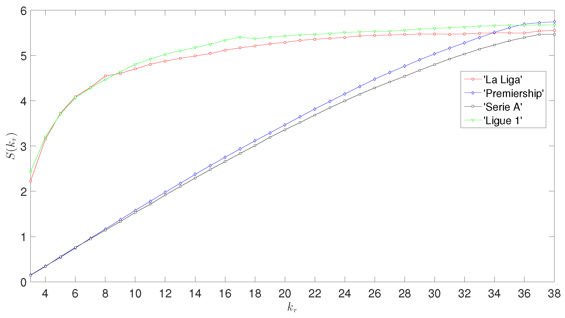
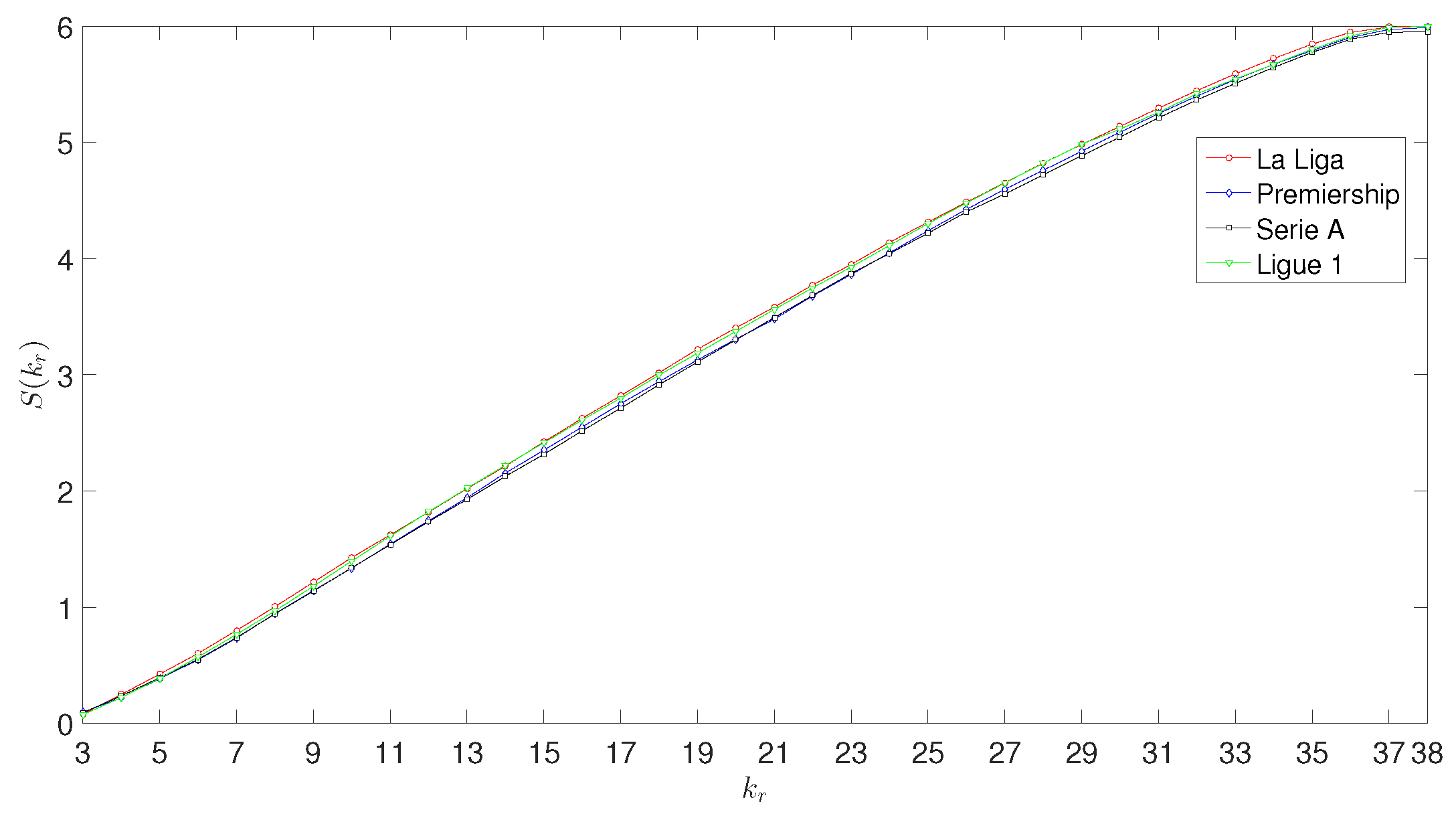
Figure 5 illustrates the evolution on the entropy, S ( k r ) versus k r = 3 , , 38 , for the PL parameters and ‘La Liga’, ‘Premiership’, ‘Serie A’ and ‘Ligue 1’. Again, we verify that the pairs P 1 and P 2 reveal similar behavior. For the pair P 1 , the entropy increases faster with k r that for the pair P 2 . This means that, in the 2018–2019 season, the Spanish and French teams started more irregular than the English and Italian ones. Nevertheless, since for all leagues, S ( k r ) converges to a similar settling value, we conclude that by the end of the season the {victory, draw, defeat} global pattern exhibited by teams in different leagues is identical.
The symmetry between the pairs P 1 and P 2 , both in the histograms of Figure 4 and the entropy evolution represented in Figure 5 opens, however, new questions. Is such duality of patterns just a casual result, or does it point towards some underlying effects ruling the dynamics of these complex systems? Additionally, can other patterns occur and what is their meaning? A future study addressing a larger number of leagues seems necessary in order to give a response to these type of questions.

3.2. The Entropy of the Ho Model

The Ho model (1f) combines both an exponential and a PL function. These functions characterize well integer- and fractional-order systems, respectively [37].
Similarly to the previous subsection, we compute the Ho parameters { a i , b i , c i } that fit the teams’ positions x i ( k ) , i = 1 , , 20 , 0 k k r , from the beginning of the season up to the round k r = 3 , , 38 . For every k r we now obtain an array of 20 × ( k r 2 ) points in a three-dimensional space. Therefore, we determine three-dimensional histograms by binning the data of each array into M × M × M = 100 × 100 × 100 bins { α j , β k , γ l } , j , k , l = 1 , , M . Finally, we calculate the Shannon entropy [35,36]:
S ( k r ) = j = 1 M k = 1 M l = 1 M P ( α j , β k , γ l ) log P ( α j , β k , γ l ) ,
where the probabilities P ( α j , β k , γ l ) are approximated by the data relative frequencies.
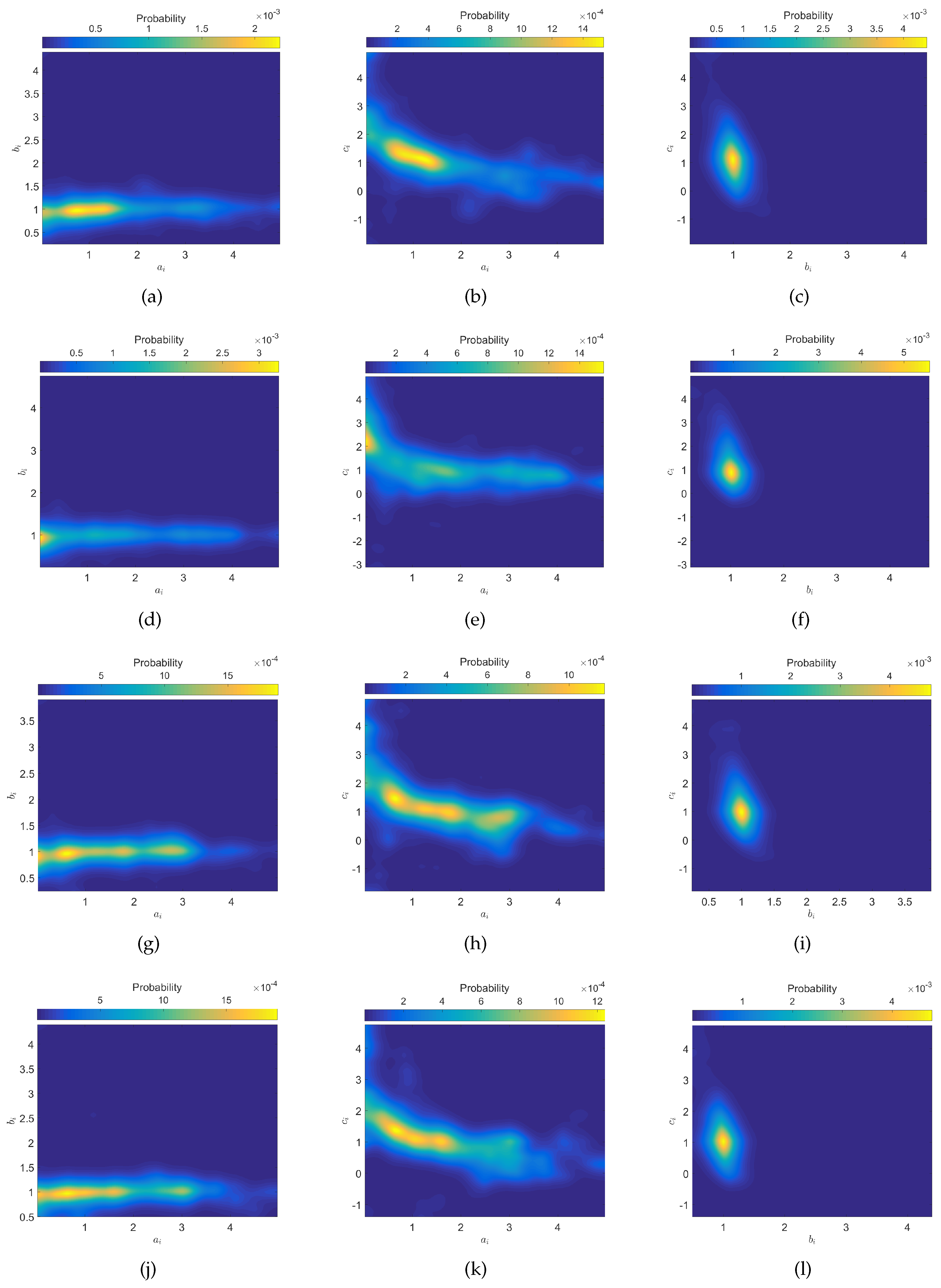
Figure 6 depicts the two-dimensional projections of the histogram of the Ho parameters, from the beginning, k r = 3 , up to the end of the 2018–2019 season, k r = 38 , for ‘La Liga’, ‘Premiership’, ‘Serie A’ and ‘Ligue 1’. Therefore, the charts represent the combination of the pairs of parameters { a i , b i } , { a i , c i } and { b i , c i } . As for the PL model, we verify that, in general, the parameters { a i , b i , c i } exhibit less dispersion for the leagues P 1 = { ‘La Liga’, ‘Ligue 1’} than for the leagues P 2 = { ‘Premiership’, ‘Serie A’}.
Figure 7 depicts the entropy, S ( k r ) versus k r = 3 , , 38 , for the Ho model parameters, and ‘La Liga’, ‘Premiership’, ‘Serie A’ and ‘Ligue 1’. We verify that S ( k r ) has now an identical behavior for all leagues, but we can still distinguish a slight difference between the pairs P 1 and P 2 .

4. Predicting the Teams’ Results

The models (1a)–(1f), introduced in Section 2, are now tested in the prediction of the teams’ results. In a first phase, we fit the models to the series x i ( k ) , i = 1 , , N , 0 k k r , and we calculate the approximation x ^ i ( k ) for each k r = 3 , , 37 . In a second phase, we extrapolate the values of x ^ i ( k + 1 ) , that is, the teams positions for every round from four to 38. Finally, in a third phase, we assess the accuracy of the values x ^ i ( k + 1 ) by means of the prediction errors E and E , where k r = 4 , , 38 .
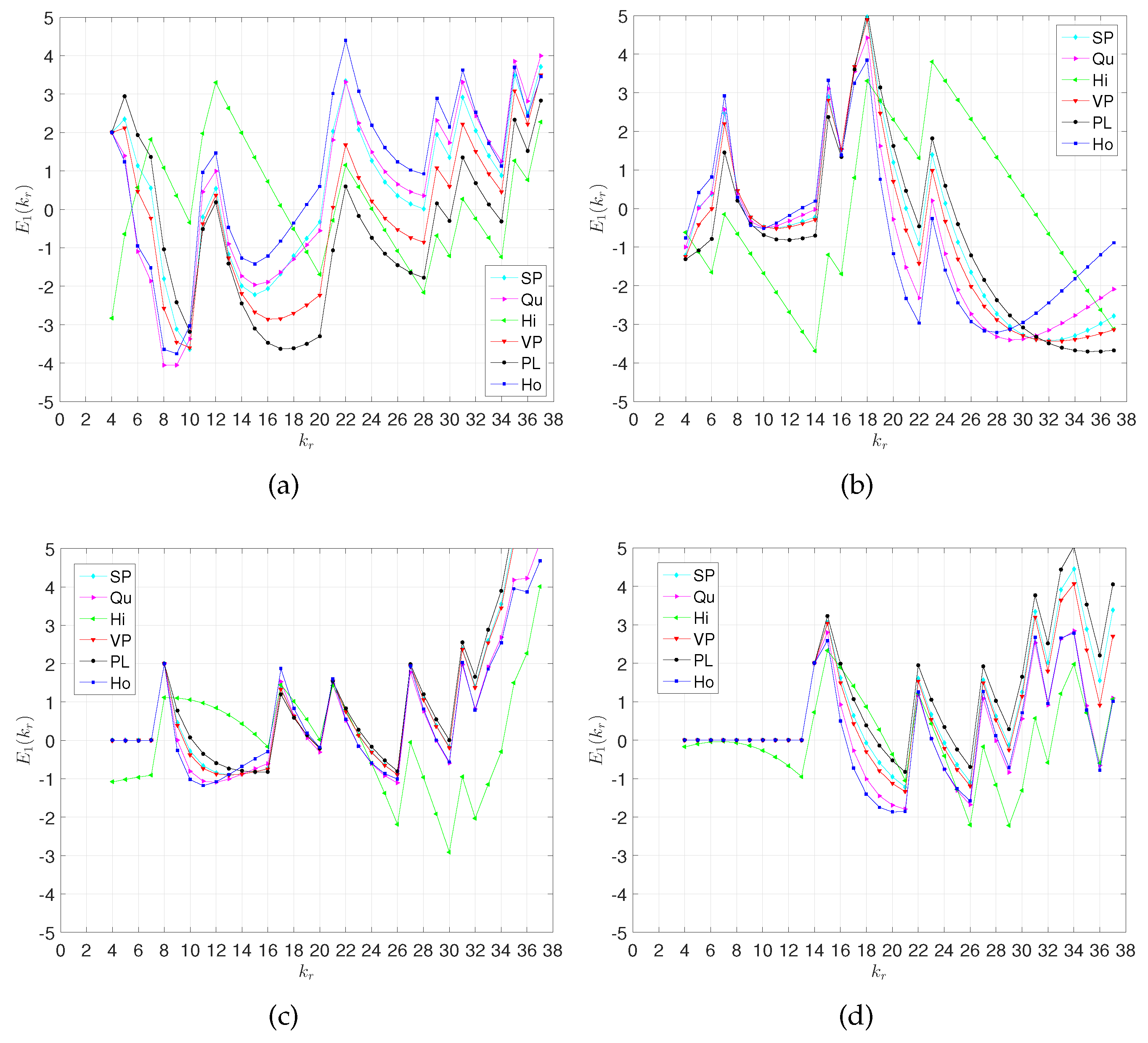
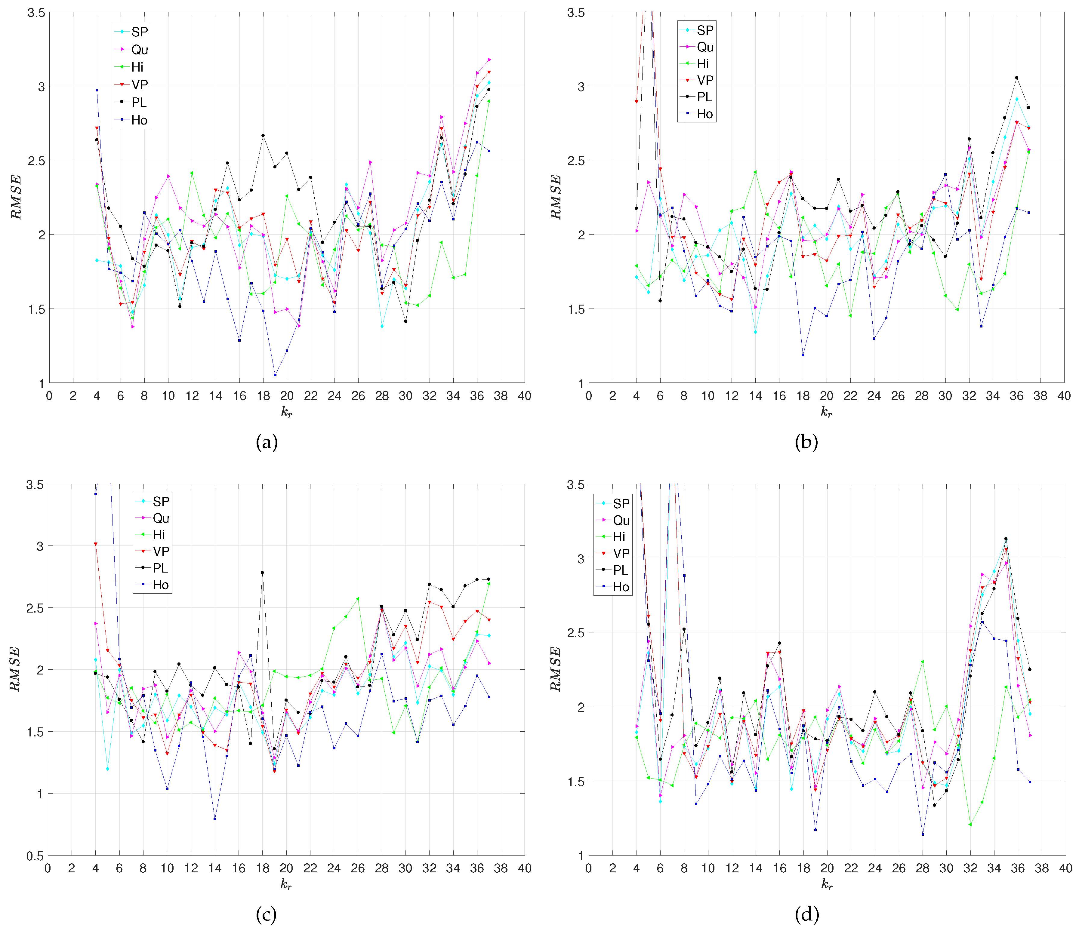
Figure 8 illustrates the error E 1 ( k r ) , k r = 4 , , 38 , obtained with the models (1a)–(1f) for the champions of the ‘La Liga’, ‘Premiership’, ‘Serie A’ and ‘Ligue 1’ in season 2018–2019, namely for the FC Barcelona, Manchester City, Juventus and Paris Saint-Germain. Figure 9 depicts E ( k r ) , k r = 4 , , 38 , for ‘La liga’, ‘Premiership’, ‘Serie A’ and ‘Ligue 1’, obtained with the six models (1a)–(1f). We verify again that, with the exception of the Hi model (1c), all other models predict well the teams’ results.
For a numerical comparison of the models accuracy, we calculate the mean and the standard deviation, μ and σ , of the E ( k r ) series and list their values in Table 2. We verify again that the Ho (1f) model leads to the best predictions. We can see that the errors are larger for the leagues in the set P 1 than for the ones in the set P 2 , meaning that the prediction is more difficult for the leagues with higher values of entropy.

5. Conclusions

We proposed a fractional systems’ perspective for analyzing soccer teams competing within a league season. Firstly, we adopted six fitting models to describe the teams’ positions along one season and interpreted the loci of the models’ parameters as a signature of the system dynamics. Secondly, we studied the entropy of the models parameters’ spatio-temporal patterns for comparing different leagues. Both approaches represent valid tools to describe the complex behavior of such challenging systems. The computational modeling unraveled patterns embedded in the data suggesting some common underlying dynamical effects in different leagues. The prediction quality of the two models, both in the perspective of each individual team and the league, along the season, was also analyzed. Nonetheless, several new questions emerged in the sequence of the statistical and entropic analysis. Is the apparent duality between the pairs P 1 and P 2 just some coincidence or do they reflect some kind of additional effects besides the standard rules of the game? The investigation of these and other questions needs the future algorithmic treatment of more data involving more seasons and leagues.

Author Contributions

A.M.L. and J.A.T.M. conceived, designed and performed the experiments, analyzed the data and wrote the paper. These authors contributed equally to this work. All authors have read and agreed to the published version of the manuscript.

Funding

This research received no external funding.

Conflicts of Interest

The authors declare no conflict of interest.

References

  1. Carling, C.; Williams, A.M.; Reilly, T. Handbook of Soccer Match Analysis: A Systematic Approach to Improving Performance; Routledge: Abingdon, UK, 2007. [Google Scholar]
  2. Giulianotti, R. Football. In The Wiley-Blackwell Encyclopedia of Globalization; Wiley: Hoboken, NJ, USA, 2012. [Google Scholar]
  3. Brocas, I.; Carrillo, J.D. Do the “three-point victory” and “golden goal” rules make soccer more exciting? J. Sport. Econ. 2004, 5, 169–185. [Google Scholar] [CrossRef] [Green Version]
  4. Miller, K.S.; Ross, B. An Introduction to the Fractional Calculus and Fractional Differential Equations; Wiley: Hoboken, NJ, USA, 1993. [Google Scholar]
  5. Tenreiro Machado, J.A.; Kiryakova, V. Recent history of the fractional calculus: Data and statistics. In Handbook of Fractional Calculus with Applications: Basic Theory; Kochubei, A., Luchko, Y., Eds.; De Gruyter: Berlin, Germany, 2019; Volume 1, pp. 1–21. [Google Scholar]
  6. Machado, J.T.; Pinto, C.M.; Lopes, A.M. A review on the characterization of signals and systems by power law distributions. Signal Process. 2015, 107, 246–253. [Google Scholar] [CrossRef]
  7. Parsa, B.; Dabiri, A.; Machado, J.A.T. Application of Variable order Fractional Calculus in Solid Mechanics. In Handbook of Fractional Calculus with Applications: Applications in Engineering, Life and Social Sciences, Part A; Baleanu, D., Lopes, A.M., Eds.; De Gruyter: Berlin, Germany, 2019; Volume 7, pp. 207–224. [Google Scholar]
  8. Machado, J.T.; Lopes, A.M. Fractional Electromagnetics. In Handbook of Fractional Calculus with Applications: Applications in Physics, Part B; Tarasov, V.E., Ed.; De Gruyter: Berlin, Germany, 2019; Volume 5, pp. 1–23. [Google Scholar]
  9. Lopes, A.M.; Machado, J. Fractional order models of leaves. J. Vib. Control. 2014, 20, 998–1008. [Google Scholar] [CrossRef] [Green Version]
  10. Machado, J.T.; Lopes, A.M. On the mathematical modeling of soccer dynamics. Commun. Nonlinear Sci. Numer. Simul. 2017, 53, 142–153. [Google Scholar] [CrossRef]
  11. Machado, J.; Mata, M.E.; Lopes, A.M. Fractional state space analysis of economic systems. Entropy 2015, 17, 5402–5421. [Google Scholar] [CrossRef] [Green Version]
  12. Valério, D.; Ortigueira, M.; Machado, J.T.; Lopes, A.M. Continuous-time fractional linear systems: Steady-state behaviour. In Handbook of Fractional Calculus with Applications: Applications in Engineering, Life and Social Sciences, Part A; Petráš, I., Ed.; De Gruyter: Berlin, Germany, 2019; Volume 6, pp. 149–174. [Google Scholar]
  13. Couceiro, M.S.; Clemente, F.M.; Martins, F.M.; Machado, J.A.T. Dynamical stability and predictability of football players: The study of one match. Entropy 2014, 16, 645–674. [Google Scholar] [CrossRef] [Green Version]
  14. Silva, P.; Duarte, R.; Esteves, P.; Travassos, B.; Vilar, L. Application of entropy measures to analysis of performance in team sports. Int. J. Perform. Anal. Sport 2016, 16, 753–768. [Google Scholar] [CrossRef]
  15. Machado, J.T.; Lopes, A.M. Multidimensional scaling analysis of soccer dynamics. Appl. Math. Model. 2017, 45, 642–652. [Google Scholar] [CrossRef]
  16. Neuman, Y.; Israeli, N.; Vilenchik, D.; Cohen, Y. The adaptive behavior of a soccer team: An entropy-based analysis. Entropy 2018, 20, 758. [Google Scholar] [CrossRef] [Green Version]
  17. Lopes, A.M.; Tenreiro Machado, J. Entropy Analysis of Soccer Dynamics. Entropy 2019, 21, 187. [Google Scholar] [CrossRef] [Green Version]
  18. Berrar, D.; Lopes, P.; Davis, J.; Dubitzky, W. Guest editorial: Special issue on machine learning for soccer. Mach. Learn. 2019, 108, 1–7. [Google Scholar] [CrossRef] [Green Version]
  19. Karlis, D.; Ntzoufras, I. Analysis of sports data by using bivariate Poisson models. J. R. Stat. Soc. Ser. D (The Stat.) 2003, 52, 381–393. [Google Scholar] [CrossRef]
  20. Baio, G.; Blangiardo, M. Bayesian hierarchical model for the prediction of football results. J. Appl. Stat. 2010, 37, 253–264. [Google Scholar] [CrossRef] [Green Version]
  21. Hvattum, L.M.; Arntzen, H. Using ELO ratings for match result prediction in association football. Int. J. Forecast. 2010, 26, 460–470. [Google Scholar] [CrossRef]
  22. Berrar, D.; Lopes, P.; Dubitzky, W. Incorporating domain knowledge in machine learning for soccer outcome prediction. Mach. Learn. 2019, 108, 97–126. [Google Scholar] [CrossRef] [Green Version]
  23. Murphy, K.P. Machine Learning: A Probabilistic Perspective; MIT Press: Cambridge, MA, USA, 2012. [Google Scholar]
  24. Van Haaren, J.; Van den Broeck, G. Relational learning for football-related predictions. In Latest Advances in Inductive Logic Programming; World Scientific: Singapore, 2015; pp. 237–244. [Google Scholar]
  25. Hubáček, O.; Šourek, G.; Železnỳ, F. Learning to predict soccer results from relational data with gradient boosted trees. Mach. Learn. 2019, 108, 29–47. [Google Scholar] [CrossRef] [Green Version]
  26. Tsokos, A.; Narayanan, S.; Kosmidis, I.; Baio, G.; Cucuringu, M.; Whitaker, G.; Király, F. Modeling outcomes of soccer matches. Mach. Learn. 2019, 108, 77–95. [Google Scholar] [CrossRef] [Green Version]
  27. Edla, D.R.; Lingras, P.; Venkatanareshbabu, K. Advances in Machine Learning and Data Science: Recent Achievements and Research Directives; Springer: Berlin, Germany, 2018. [Google Scholar]
  28. Abu-Mostafa, Y.S.; Magdon-Ismail, M.; Lin, H.T. Learning from Data; AMLBook: New York, NY, USA, 2012. [Google Scholar]
  29. Lawson, C.L.; Hanson, R.J. Solving Least Squares Problems; SIAM: Philadelphia, PA, USA, 1974; Volume 161. [Google Scholar]
  30. Draper, N.R.; Smith, H.; Pownell, E. Applied Regression Analysis; Wiley: New York, NY, USA, 1966; Volume 3. [Google Scholar]
  31. Lopes, A.; Tenreiro Machado, J.; Galhano, A. Empirical laws and foreseeing the future of technological progress. Entropy 2016, 18, 217. [Google Scholar] [CrossRef] [Green Version]
  32. Lopes, A.; Tenreiro Machado, J. Complexity Analysis of Global Temperature Time Series. Entropy 2018, 20, 437. [Google Scholar] [CrossRef] [Green Version]
  33. Machado, J.T.; Lopes, A.M. The persistence of memory. Nonlinear Dyn. 2015, 79, 63–82. [Google Scholar] [CrossRef] [Green Version]
  34. Machado, J.; Lopes, A.M. Analysis of natural and artificial phenomena using signal processing and fractional calculus. Fract. Calc. Appl. Anal. 2015, 18, 459–478. [Google Scholar] [CrossRef] [Green Version]
  35. Shannon, C. A Mathematical Theory of Communication. Bell Syst. Tech. J. 1948, 27, 379–423. [Google Scholar] [CrossRef] [Green Version]
  36. Jaynes, E. Information Theory and Statistical Mechanics. Phys. Rev. 1957, 106, 620–630. [Google Scholar] [CrossRef]
  37. Pinto, C.M.; Lopes, A.M.; Machado, J.T. A review of power laws in real life phenomena. Commun. Nonlinear Sci. Numer. Simul. 2012, 17, 3558–3578. [Google Scholar] [CrossRef] [Green Version]
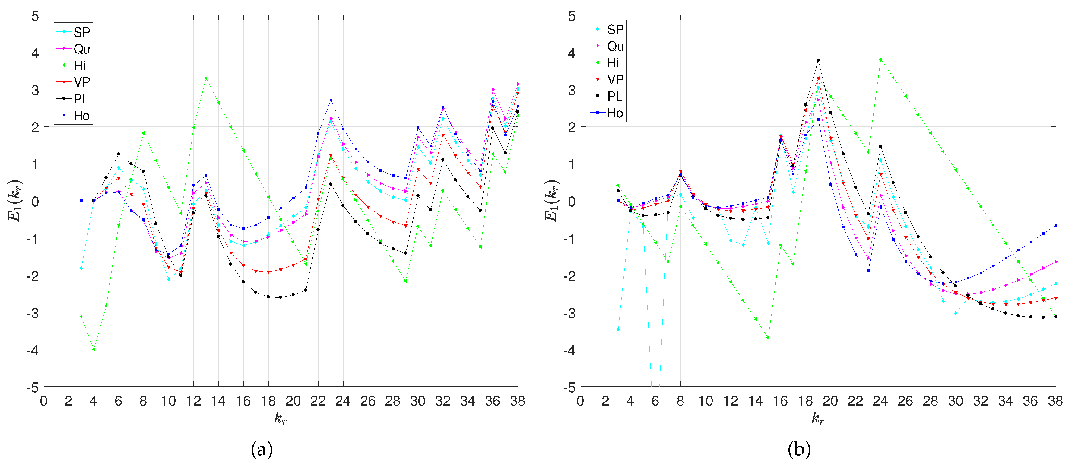
Figure 1. The error E 1 ( k r ) , k r = 3 , , 38 , for the models (1a)–(1f), during the season 2018–2019: (a) FC Barcelona; (b) Manchester City.
Symmetry 12 00356 g001
Figure 2. The error E ( k r ) , k r = 3 , , 38 , for the models (1a)–(1f), during the season 2018–2019: (a) ‘La liga’; (b) ‘Premiership’.
Symmetry 12 00356 g002
Figure 3. Locus of the the models parameters for the 2018–2019 champions of ‘La Liga’ and ‘Premiership’: (a) PL model for FC Barcelona; (b) Ho model for FC Barcelona; (c) PL model for Manchester City; (d) Ho model for Manchester City. The point labels denote k r = 3 , , 38 .
Symmetry 12 00356 g003
Figure 4. Histograms of the PL parameters { a i , b i } from the beginning, k r = 3 , up to the end of the 2018–2019 season, k r = 38 , and the leagues: (a) ‘La Liga’; (b) ‘Premiership’; (c) ‘Serie A’; (d) ‘Ligue 1’.
Symmetry 12 00356 g004
Figure 5. Evolution of the entropy S ( k r ) versus k r = 3 , , 38 , for the PL parameters and the ‘La Liga’, ‘Premiership’, ‘Serie A’ and ‘Ligue 1’, during the season 2018–2019.
Symmetry 12 00356 g005
Figure 6. The two-dimensional projections of the histograms of the Ho parameters, from the beginning, k r = 3 , up to the end of the 2018–2019 season, and the leagues: (ac) ‘La Liga’; (df) ‘Premiership’; (gi) ‘Serie A’; (jl) ‘Ligue 1’. The charts represent the combination of the pairs of parameters { a i , b i } , { a i , c i } and { b i , c i } .
Symmetry 12 00356 g006
Figure 7. Evolution of the entropy S ( k r ) versus k r = 3 , , 38 , for the Ho model parameters and the leagues ‘La Liga’, ‘Premiership’, ‘Serie A’ and ‘Ligue 1’, during the season 2018–2019.
Symmetry 12 00356 g007
Figure 8. The error E 1 ( k r ) , k r = 4 , , 38 , for the models (1a)–(1f), during the season 2018–2019: (a) FC Barcelona; (b) Manchester City; (c) Juventus; (d) Paris Saint-Germain.
Symmetry 12 00356 g008
Figure 9. The error E ( k r ) , k r = 4 , , 38 , for the models (1a)–(1f), during the season 2018–2019: (a) ‘La liga’; (b) ‘Premiership’; (c) ‘Serie A’; (d) ‘Ligue 1’.
Symmetry 12 00356 g009
Table 1. The mean and standard deviation, μ and σ , of the E ( k r ) series for the four leagues and the models (1a)–(1f), during the season 2018–2019.
SPQuHiVPPLHo
‘La Liga’ μ 1.31821.18321.58521.20511.41181.0782
σ 0.49860.54410.25920.56070.57460.4736
‘Premiership’ μ 1.23541.10821.50611.16991.33681.0394
σ 0.52330.55290.22400.59840.54960.5112
‘Serie A’ μ 1.17491.05741.57831.15961.38001.0045
σ 0.44260.48650.29660.59770.59630.4251
‘Ligue 1’ μ 1.30351.20531.65621.23131.43571.1333
σ 0.51550.61440.30930.60800.56270.5813
Table 2. The mean and standard deviation, μ and σ , of the E ( k r ) for the six models (1a)–(1f) and season 2018–2019.
SPQuHiVPPLHo
‘La Liga’ μ 2.01372.11771.93972.06042.16311.9172
σ 0.38070.43390.30760.39450.36840.4173
‘Premiership’ μ 1.97651.95431.99362.08602.09261.9036
σ 0.55190.40190.21980.63360.52260.6672
‘Serie A’ μ 1.80931.87171.87651.94622.04681.7322
σ 0.29300.27640.30420.42160.41390.5888
‘Ligue 1’ μ 2.04072.10221.99122.14002.19351.9337
σ 0.32260.28350.26570.46830.46530.5536