A Shift-Dependent Measure of Extended Cumulative Entropy and Its Applications in Blind Image Quality Assessment


Abstract
1. Introduction
2. Some Results on WECE and Its Dynamic Past Version
- i.
- If X is uniformly distributed in , then,
- ii.
- If X has the distribution with , then for we have
- iii.
- If X has an inverse Weibull distribution with then
- iv.
- If , with and , then .
- X is smaller than Y in the usual stochastic order (denoted by ) if for all x.
- X is smaller than Y in the likelihood ration ordering (denoted by ) if is increasing in x;
- X is smaller than Y in the reversed hazard rate order, denoted by , if for all x;
- X is smaller than Y in the decreasing convex order, denoted by , if for all decreasing convex functions ϕ such that the expectations exist;
- X is smaller than Y in the dispersive order, denoted by , if where and are right continuous inverses of F and G, respectively;
- A non-negative random variable X is said to have a decreasing reversed hazard rate (DRHR) if is decreasing in x;
- A non-negative random variable X is said to have a decreasing reversed hazard rate average (DRHRA) if is a decreasing function in . Note that DRHR classes of distributions are included in DRHRA classes of distributions.
- i.
- ii.
- iii.
3. Properties of Conditional WECE
- i.
- ii.
- (i)
- By using the Markov property and definition of , the result follows.
- (ii)
- Let and , then from (20) we haveand the result follows. □
4. Relationships with Other Reliability Functions
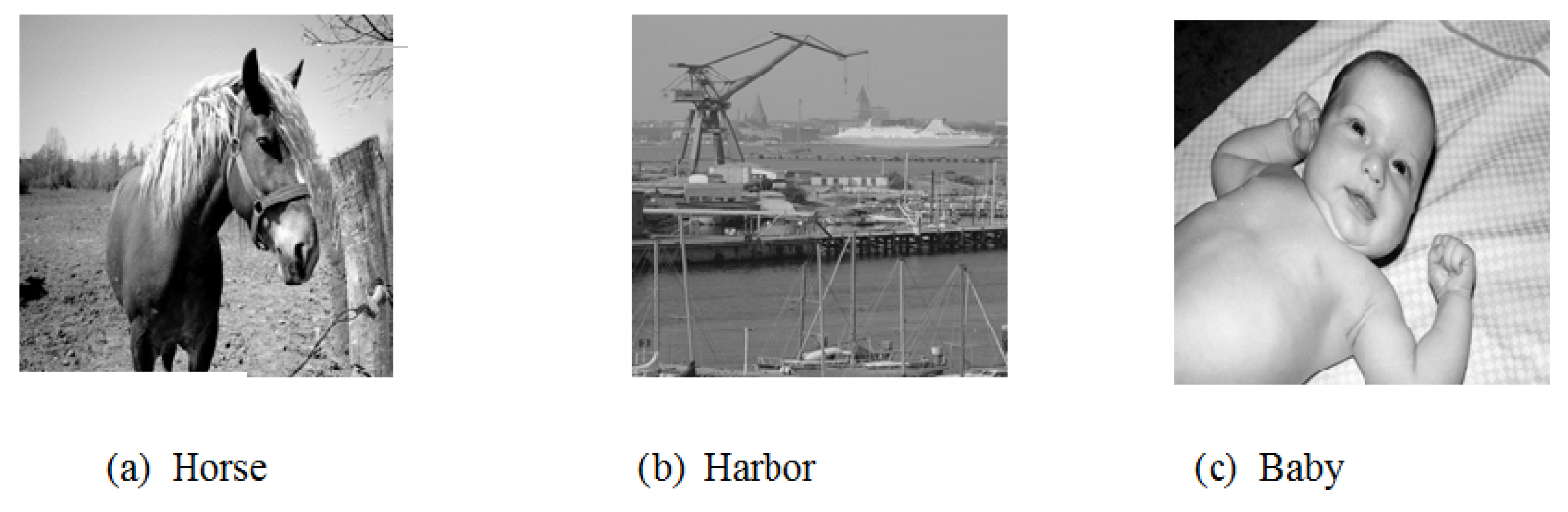
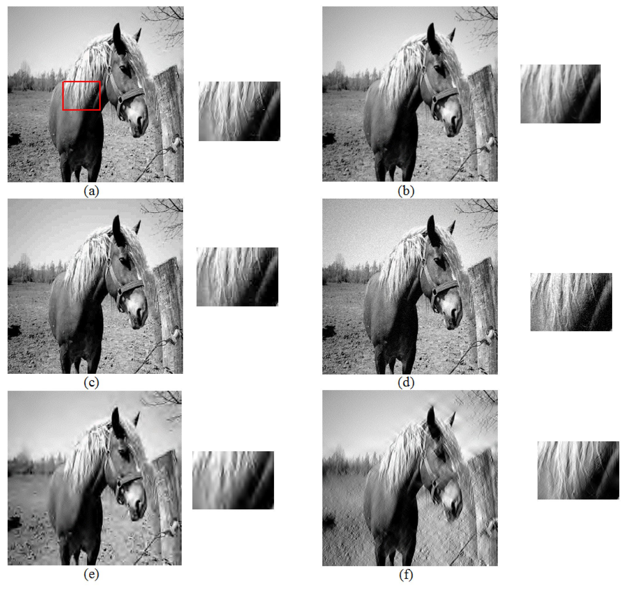
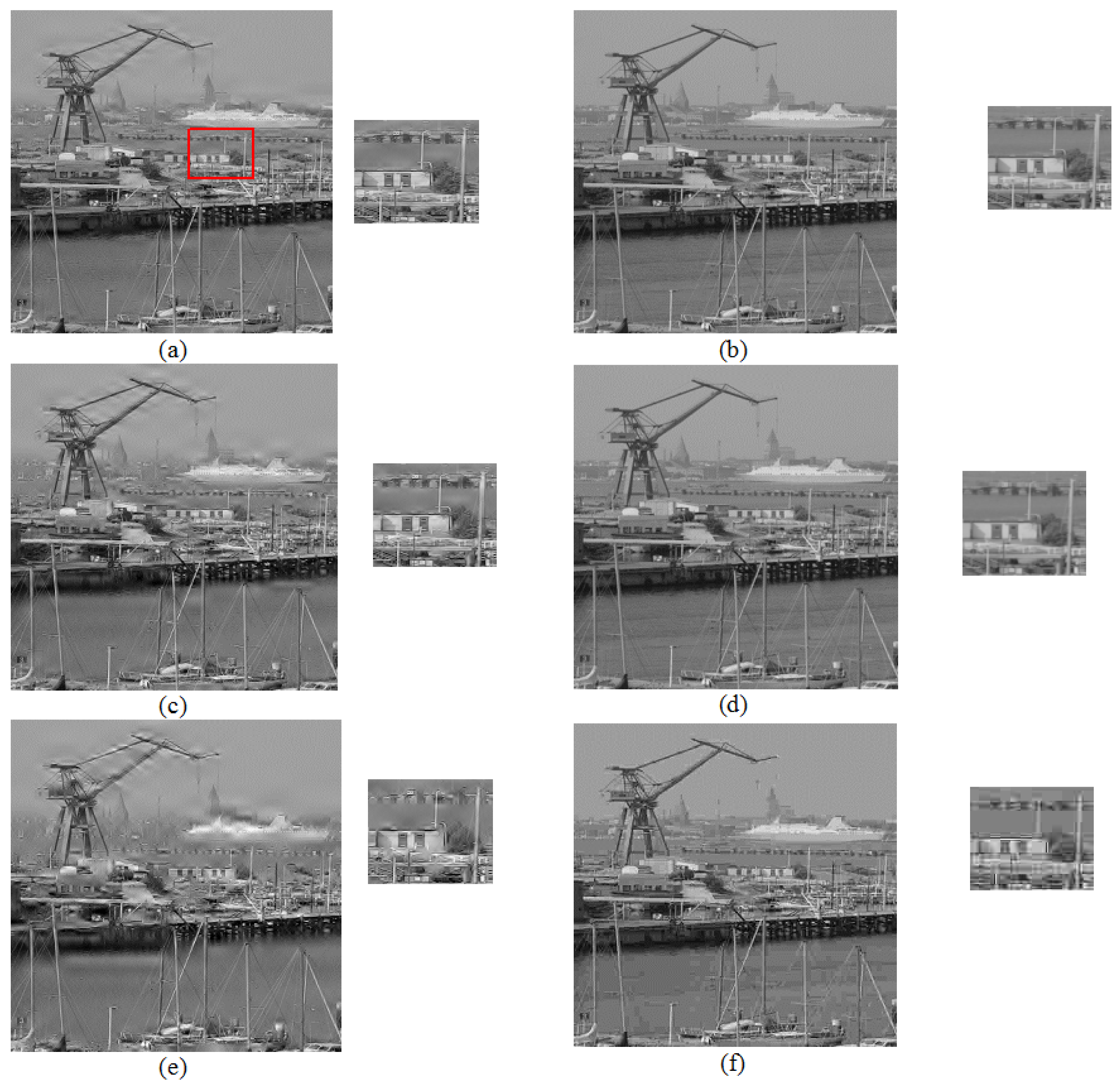
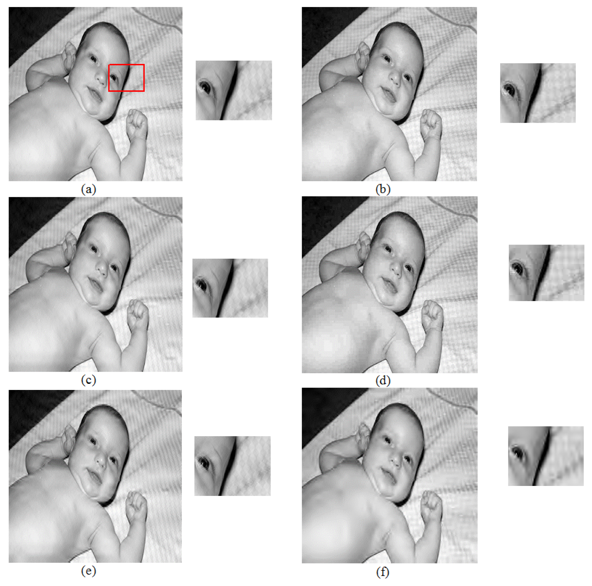
5. Application of in Blind Image Quality Assessment
6. Conclusions
Author Contributions
Funding
Acknowledgments
Conflicts of Interest
References
- Shannon, C.A. Mathematical theory of communication. Bell Syst. Tech. J. 1948, 27, 379–432. [Google Scholar] [CrossRef]
- Renyi, A. On measures of entropy and information. In Proceedings of the Fourth Berkeley Symposium on Mathematical Statistics and Probability; University of California Press: Berkeley, CA, USA, 1961; pp. 547–561. [Google Scholar]
- Rao, M.; Chen, Y.; Vemuri, B.C.; Wang, F. Cumulative Residual Entropy: A New Measure of Information. IEEE Trans. Inf. Theory 2004, 50, 1220–1228. [Google Scholar] [CrossRef]
- Di Crescenzo, A.; Longobardi, M. On cumulative entropies. J. Stat. Plan. Inference 2009, 139, 4072–4087. [Google Scholar] [CrossRef]
- Di Crescenzo, A.; Toomaj, A. Extension of the past lifetime and its connection to the cumulative entropy. J. Appl. Probab. 2015, 52, 1156–1174. [Google Scholar] [CrossRef][Green Version]
- Psarrakos, G.; Navarro, J. Generalized cumulative residual entropy and record values. Metrika 2013, 76, 623–640. [Google Scholar] [CrossRef]
- Calì, C.; Longobardi, M.; Psarrakos, G. A family of weighted distributions based on the mean inactivity time and cumulative past entropies. Ricerche di Matematica 2019. [Google Scholar] [CrossRef]
- Moharana, R.; Kayal, S. On Weighted Extended Cumulative Residual Entropy of k-th Upper Record. In Digital Business. Lecture Notes on Data Engineering and Communications Technologies; Patnaik, S., Yang, X.S., Tavana, M., Popentiu-Vlădicescu, F., Qiao, F., Eds.; Springer: Cham, Switzerland, 2019; Volume 21. [Google Scholar]
- Tahmasebi, S.; Longobardi, M.; Foroghi, F.; Lak, F. An extension of weighted generalized cumulative past measure of information. Ricerche di Matematica 2019. [Google Scholar] [CrossRef]
- Dziubdziela, W.; Kopocinski, B. Limiting properties of the k-th record value. Zastos. Math. 1976, 15, 187–190. [Google Scholar] [CrossRef]
- Tahmasebi, S.; Eskandarzadeh, M. Generalized cumulative entropy based on kth lower record values. Stat. Probab. Lett. 2017, 126, 164–172. [Google Scholar] [CrossRef]
- Olshausen, B.A.; Field, D.J. Emergence of simple-cell receptive field properties by learning a sparse code for natural images. Nature 1996, 381, 607. [Google Scholar] [CrossRef]
- Shaked, M.; Shanthikumar, J.G. Stochastic Orders; Springer: New York, NY, USA, 2007. [Google Scholar]
- Klein, I.; Mangold, B.; Doll, M. Cumulative paired ϕ-entropy. Entropy 2016, 18, 248. [Google Scholar] [CrossRef]
- Kayal, S.; Moharana, S.R. A shift-dependent generalized cumulative entropy of order n. Commun. Stat. Simul. Comput. 2018. [Google Scholar] [CrossRef]
- Bdair, O.M.; Raqab, M.Z. Sharp upper bounds for the mean residual waiting time of records. Statistics 2012, 46, 69–84. [Google Scholar] [CrossRef]
- Gabarda, S.; Cristobal, G. Blind image quality assessment through Anisotropy. J. Opt. Soc. Am. A 2007, 24, B42–B51. [Google Scholar] [CrossRef]
- Chandler, D.M.; Hemami, S.S. VSNR: A Wavelet-Based Visual Signal-to-Noise Ratio for Natural Images. IEEE Trans. Image Process. 2007, 16, 2284–2298. [Google Scholar] [CrossRef]
- Chandler, D.M.; Hemami, S.S. A57 Image Quality Database. 2018. Available online: http://vision.eng.shizuoka.ac.jp/mod/page/view.php?id=26 (accessed on 22 December 2019).
- Mannos, J.L.; Sakrison, D.J. The effects of a visual fidelity criterion on the encoding of image. IEEE Trans. Inf. Theory 1974, IT-20, 525–535. [Google Scholar] [CrossRef]
- Wang, Z.; Bovik, A. A universal image quality index. IEEE Signal Process. Lett. 2002, 9, 81–84. [Google Scholar] [CrossRef]
- Damera-Venkata, N.; Kite, T.D.; Geisler, W.S.; Evans, B.L.; Bovik, A.C. Image quality assessment based on a degradation model. IEEE Trans. Image Process. 2000, 9, 636–650. [Google Scholar] [CrossRef]
- Wang, Z.; Bovik, A.; Sheikh, H.; Simoncelli, E. Image quality assessment: From error visibility to structural similarity. IEEE Trans. Image Process. 2004, 13, 600–612. [Google Scholar] [CrossRef]
- Sheikh, H.R.; Bovik, A.C. Image information and visual quality. IEEE Trans. Image Process. 2006, 15, 430–444. [Google Scholar] [CrossRef]
- Shi, Z.; Zhang, J.; Cao, Q.; Pang, K.; Luo, T. Full-reference image quality assessment based on image segmentation with edge feature. Signal Process. 2018, 145, 99–105. [Google Scholar] [CrossRef]
- Fieller, E.C.; Hartley, H.O.; Pearson, E.S. Tests for rank correlation coefficients. I. Biometrika 1957, 44, 470–481. [Google Scholar] [CrossRef]


| Image | Distortion | Full-Reference Image Quality Metric | Blind Image Quality Metric | ||||||
|---|---|---|---|---|---|---|---|---|---|
| SSIM | VIF | NQM | UQI | PSNR | VSNR | Rnyi-AIQ | WECE-AIQ | ||
| Horse (GQ) | FLT | 0.933 | 0.570 | 19.391 | 0.833 | 28.983 | 20.597 | 0.00503661 | 0.00128575 |
| JPG | 0.970 | 0.572 | 33.125 | 0.694 | 29.003 | 30.095 | 0.00564478 | 0.00114628 | |
| JP2 | 0.946 | 0.427 | 30.446 | 0.656 | 28.870 | 27.700 | 0.0064663 | 0.00124661 | |
| DCQ | 0.962 | 0.508 | 31.849 | 0.685 | 28.891 | 36.342 | 0.00577385 | 0.00112959 | |
| BLR | 0.974 | 0.637 | 38.456 | 0.816 | 29.056 | 26.884 | 0.00565214 | 0.0013568 | |
| AGWN | 0.907 | 0.559 | 29.675 | 0.659 | 28.822 | 28.584 | 0.00399926 | 0.00072772 | |
| Horse (MQ) | FLT | 0.903 | 0.513 | 17.146 | 0.799 | 26.734 | 17.934 | 0.0054712 | 0.0011785 |
| JPG | 0.926 | 0.374 | 28.033 | 0.589 | 26.701 | 23.736 | 0.0069904 | 0.0014497 | |
| JP2 | 0.895 | 0.289 | 26.124 | 0.558 | 26.545 | 23.230 | 0.0057527 | 0.0013887 | |
| DCQ | 0.938 | 0.416 | 31.940 | 0.624 | 26.590 | 27.577 | 0.0052392 | 0.0013404 | |
| BLR | 0.944 | 0.498 | 34.419 | 0.702 | 26.733 | 22.566 | 0.0037091 | 0.0005268 | |
| AGWN | 0.861 | 0.473 | 27.612 | 0.603 | 26.496 | 25.518 | 0.0054970 | 0.0016277 | |
| Horse (LQ) | FLT | 0.840 | 0.437 | 13.808 | 0.709 | 23.777 | 14.561 | 0.00652794 | 0.0017846 |
| JPG | 0.786 | 0.176 | 19.448 | 0.400 | 23.622 | 17.092 | 0.00549665 | 0.0016539 | |
| JP2 | 0.753 | 0.122 | 19.999 | 0.371 | 23.230 | 15.921 | 0.0070989 | 0.0014571 | |
| DCQ | 0.781 | 0.137 | 23.099 | 0.396 | 23.213 | 15.997 | 0.00697058 | 0.0012112 | |
| BLR | 0.835 | 0.262 | 25.978 | 0.487 | 23.725 | 16.456 | 0.00395791 | 0.0011317 | |
| AGWN | 0.777 | 0.363 | 24.709 | 0.513 | 23.300 | 21.530 | 0.00318548 | 0.0003756 | |
| Harbor (GQ) | FLT | 0.935 | 0.608 | 14.953 | 0.772 | 31.098 | 18.362 | 0.00317073 | 0.00113086 |
| JPG | 0.984 | 0.735 | 28.190 | 0.672 | 31.149 | 31.659 | 0.00302575 | 0.00103601 | |
| JP2 | 0.949 | 0.493 | 24.223 | 0.585 | 31.118 | 24.349 | 0.00303644 | 0.00113519 | |
| DCQ | 0.975 | 0.649 | 26.711 | 0.663 | 31.202 | 35.532 | 0.00313986 | 0.00110450 | |
| BLR | 0.989 | 0.769 | 36.825 | 0.880 | 31.211 | 29.284 | 0.00226195 | 0.00151543 | |
| AGWN | 0.934 | 0.640 | 26.318 | 0.658 | 31.097 | 26.079 | 0.00287300 | 0.000939305 | |
| Harbor (MQ) | FLT | 0.906 | 0.545 | 12.597 | 0.721 | 28.740 | 15.843 | 0.0031356 | 0.0010805 |
| JPG | 0.968 | 0.589 | 26.207 | 0.608 | 28.909 | 26.549 | 0.00292496 | 0.00115297 | |
| JP2 | 0.918 | 0.363 | 21.363 | 0.515 | 28.792 | 21.245 | 0.002908160 | 0.00111366 | |
| DCQ | 0.959 | 0.540 | 26.106 | 0.592 | 28.858 | 30.429 | 0.0030507 | 0.00119234 | |
| BLR | 0.979 | 0.684 | 35.112 | 0.784 | 28.908 | 25.740 | 0.00195757 | 0.001470153 | |
| AGWN | 0.895 | 0.552 | 24.244 | 0.607 | 28.724 | 23.095 | 0.00275998 | 0.001070499 | |
| Harbor (LQ) | FLT | 0.854 | 0.462 | 9.254 | 0.651 | 25.556 | 12.315 | 0.00277902 | 0.00110425 |
| JPG | 0.896 | 0.302 | 18.306 | 0.439 | 25.502 | 18.411 | 0.002717076 | 0.0014915792 | |
| JP2 | 0.843 | 0.204 | 16.939 | 0.384 | 25.569 | 16.309 | 0.00231397 | 0.0010248261 | |
| DCQ | 0.931 | 0.395 | 24.526 | 0.490 | 25.610 | 27.498 | 0.002142166 | 0.0010449862 | |
| BLR | 0.939 | 0.490 | 30.010 | 0.576 | 25.802 | 19.524 | 0.001351146 | 0.0014994589 | |
| AGWN | 0.818 | 0.438 | 21.897 | 0.526 | 25.536 | 19.318 | 0.002607232 | 0.0005917831 | |
| Baby (GQ) | FLT | 0.948 | 0.614 | 22.824 | 0.843 | 34.485 | 23.352 | 0.001806857 | 0.000464815 |
| JPG | 0.955 | 0.504 | 29.818 | 0.718 | 34.528 | 27.700 | 0.001632599 | 0.000500301 | |
| JP2 | 0.945 | 0.413 | 28.877 | 0.675 | 34.504 | 26.049 | 0.001734634 | 0.00034369 | |
| DCQ | 0.968 | 0.547 | 30.761 | 0.751 | 34.522 | 28.767 | 0.001640073 | 0.000445138 | |
| BLR | 0.979 | 0.637 | 34.323 | 0.824 | 34.636 | 26.431 | 0.001428632 | 0.000429976 | |
| AGWN | 0.963 | 0.716 | 32.966 | 0.732 | 34.564 | 31.574 | 0.00170072 | 0.000383635 | |
| Baby (MQ) | FLT | 0.932 | 0.573 | 21.512 | 0.802 | 32.828 | 21.422 | 0.001849179 | 0.000506972 |
| JPG | 0.919 | 0.376 | 26.591 | 0.630 | 32.738 | 24.065 | 0.001550735 | 0.000520883 | |
| JP2 | 0.918 | 0.307 | 26.283 | 0.611 | 32.759 | 23.314 | 0.001649043 | 0.000329263 | |
| DCQ | 0.938 | 0.365 | 27.239 | 0.661 | 32.846 | 24.059 | 0.00159274 | 0.0003811 | |
| BLR | 0.964 | 0.530 | 30.984 | 0.769 | 32.931 | 23.131 | 0.001232089 | 0.00038633 | |
| AGWN | 0.946 | 0.647 | 31.594 | 0.665 | 32.740 | 29.220 | 0.001609792 | 0.000381473 | |
| Baby (LQ) | FLT | 0.907 | 0.523 | 19.740 | 0.735 | 30.772 | 19.064 | 0.001757395 | 0.000498084 |
| JPG | 0.859 | 0.264 | 22.941 | 0.507 | 30.722 | 20.583 | 0.001516522 | 0.001729756 | |
| JP2 | 0.877 | 0.222 | 23.077 | 0.529 | 30.794 | 19.833 | 0.001483539 | 0.0046381869 | |
| DCQ | 0.915 | 0.283 | 26.433 | 0.613 | 30.803 | 19.935 | 0.001341795 | 0.0042625907 | |
| BLR | 0.935 | 0.402 | 26.743 | 0.688 | 31.012 | 19.711 | 0.000895241 | 0.003490746 | |
| AGWN | 0.916 | 0.561 | 30.352 | 0.581 | 30.740 | 26.674 | 0.001570303 | 0.000022357 | |
| Image | Blind Image Quality Index | Full-Reference Image Quality Metric | |||||
|---|---|---|---|---|---|---|---|
| SSIM | VIF | NQM | UQI | PSNR | VSNR | ||
| Horse (GQ) | Rnyi-AIQ | 0.485 | −0.428 | 0.42 | −0.371 | 0.085 | 0.2 |
| WECE - AIQ | 0.485 | 0.485 | 0.257 | 0.6 | 0.714 | −0.771 | |
| Horse (MQ) | Rnyi-AIQ | 0.028 | −0.485 | −0.314 | −0.257 | 0.028 | −0.028 |
| WECE -AIQ | 0.085 | 0.142 | −0.485 | 0.314 | 0.485 | −0.542 | |
| Horse (LQ) | Rnyi-AIQ | −0.257 | −0.657 | −0.485 | −0.657 | −0.428 | −0.771 |
| WECE -AIQ | 0.428 | 0.028 | −0.942 | 0.028 | 0.371 | −0.657 | |
| Harbor (GQ) | Rnyi-AIQ | −0.371 | −0.714 | −0.714 | −0.314 | −0.257 | −0.257 |
| WECE -AIQ | 0.485 | −0.028 | 0.085 | 0.257 | 0.257 | −0.257 | |
| Harbor (MQ) | Rnyi-AIQ | −0.257 | −0.485 | −0.542 | −0.142 | −0.085 | −0.085 |
| WECE -AIQ | 0.942 | 0.314 | 0.771 | 0.257 | 0.828 | 0.657 | |
| Harbor (LQ) | Rnyi-AIQ | −0.714 | −0.2 | −0.828 | 0.085 | −0.257 | −0.714 |
| WECE -AIQ | 0.714 | 0.2 | 0.085 | 0.142 | −0.028 | −0.028 | |
| Baby (GQ) | Rnyi-AIQ | −0.771 | −0.142 | −0.7714 | 0.028 | −0.828 | −0.428 |
| WECE -AIQ | −0.142 | −0.2 | −0.028 | −0.6 | 0.085 | 0.657 | |
| Baby (MQ) | Rnyi-AIQ | −0.485 | 0.085 | −0.6 | 0.085 | −0.2 | −0.257 |
| WECE -AIQ | −0.085 | −0.485 | −0.028 | −0.314 | 0.085 | −0.028 | |
| Baby (LQ) | Rnyi-AIQ | −0.371 | 0.428 | −0.428 | 0.028 | −0.771 | 0.085 |
| WECE -AIQ | 0.314 | 0.314 | −0.2 | 0.6 | 0.257 | −0.542 | |
| Image | Image Quality Index | Full-Reference Image Quality Index | |||||
|---|---|---|---|---|---|---|---|
| SSIM | VIF | NQM | UQI | PSNR | VSNR | ||
| Horse (GQ) | SSIM | 1 | 0.542857 | 0.942857 | 0.314286 | 0.828571 | 0.142857 |
| VIF | 0.542857 | 1 | 0.485714 | 0.771429 | 0.828571 | −0.31429 | |
| NQM | 0.942857 | 0.485714 | 1 | 0.085714 | 0.657143 | 0.314286 | |
| UQI | 0.314286 | 0.771429 | 0.085714 | 1 | 0.771429 | −0.48571 | |
| PSNR | 0.828571 | 0.828571 | 0.657143 | 0.771429 | 1 | −0.25714 | |
| VSNR | 0.142857 | −0.31429 | 0.314286 | −0.48571 | −0.25714 | 1 | |
| Horse (MQ) | SSIM | 1 | 0.2 | 0.771429 | 0.428571 | 0.6 | −0.08571 |
| VIF | 0.2 | 1 | −0.02857 | 0.942857 | 0.6 | −0.48571 | |
| NQM | 0.771429 | −0.02857 | 1 | 0.085714 | 0.028571 | 0.371429 | |
| UQI | 0.428571 | 0.942857 | 0.085714 | 1 | 0.714286 | −0.42857 | |
| PSNR | 0.6 | 0.6 | 0.028571 | 0.714286 | 1 | −0.71429 | |
| VSNR | −0.08571 | −0.48571 | 0.371429 | −0.42857 | −0.71429 | 1 | |
| Horse (LQ) | SSIM | 1 | 0.657143 | −0.25714 | 0.657143 | 0.828571 | −0.25714 |
| VIF | 0.657143 | 1 | −0.08571 | 1 | 0.771429 | 0.085714 | |
| NQM | −0.25714 | −0.08571 | 1 | −0.08571 | −0.25714 | 0.542857 | |
| UQI | 0.657143 | 1 | −0.08571 | 1 | 0.771429 | 0.085714 | |
| PSNR | 0.828571 | 0.771429 | −0.25714 | 0.771429 | 1 | −0.14286 | |
| VSNR | −0.25714 | 0.085714 | 0.542857 | 0.085714 | −0.14286 | 1 | |
© 2020 by the authors. Licensee MDPI, Basel, Switzerland. This article is an open access article distributed under the terms and conditions of the Creative Commons Attribution (CC BY) license (http://creativecommons.org/licenses/by/4.0/).
Share and Cite
Tahmasebi, S.; Keshavarz, A.; Longobardi, M.; Mohammadi, R. A Shift-Dependent Measure of Extended Cumulative Entropy and Its Applications in Blind Image Quality Assessment. Symmetry 2020, 12, 316. https://doi.org/10.3390/sym12020316
Tahmasebi S, Keshavarz A, Longobardi M, Mohammadi R. A Shift-Dependent Measure of Extended Cumulative Entropy and Its Applications in Blind Image Quality Assessment. Symmetry. 2020; 12(2):316. https://doi.org/10.3390/sym12020316
Chicago/Turabian StyleTahmasebi, Saeid, Ahmad Keshavarz, Maria Longobardi, and Reza Mohammadi. 2020. "A Shift-Dependent Measure of Extended Cumulative Entropy and Its Applications in Blind Image Quality Assessment" Symmetry 12, no. 2: 316. https://doi.org/10.3390/sym12020316
APA StyleTahmasebi, S., Keshavarz, A., Longobardi, M., & Mohammadi, R. (2020). A Shift-Dependent Measure of Extended Cumulative Entropy and Its Applications in Blind Image Quality Assessment. Symmetry, 12(2), 316. https://doi.org/10.3390/sym12020316