Abstract
Proteins with a high degree of sequence similarity representing different structures provide a key to understand how protein sequence codes for 3D structure. An analysis using the fuzzy oil drop model was carried out on two pairs of proteins with different secondary structures and with high sequence identities. It has been shown that distributions of hydrophobicity for these proteins are approximated well using single 3D Gaussian function. In other words, the similar sequences fold into different 3D structures, however, alternative structures also have symmetric and monocentric hydrophobic cores. It should be noted that a significant change in the helical to beta-structured form in the N-terminal section takes places in the fragment much preceding the location of the mutated regions. It can be concluded that the final structure is the result of a complicated synergy effect in which the whole chain participates simultaneously.
Keywords:
homology; protein structure; hydrophobic core; hydrophobicity; synergy; spherical symmetry 1. Introduction
The mechanism of the protein folding process is still a puzzle despite intensive research in this direction [1]. Protein folding issues cannot be discussed without taking into account such milestones as Levinthal’s paradox [2,3,4,5,6,7], Anfinsen’s folding research [8,9] or the introduction of the concept of intermediates in the process of protein folding [10]. Early studies on the structuring of micelles in the aquatic environment associated with the process of shaping protein structure drew attention to the impact of the environment [11,12,13]. The concept of hydrophobic interactions unnoticed by quantum chemistry has become one of the decisive factors involved in protein structuring [14,15,16]. The Levinthal paradox in the era of protein simulation and prediction takes the form of the multiple minima problem [17], in which structure prediction techniques assume the evolutionary nature of structure changes and use homology modelling [18]. The ab initio methods, on the other hand, look for simplified forms of the starting structure and a simplified form of force field representation [19].
Progress in this field is closely monitored through the CASP – Critical Assessment of Structure Prediction project [20], where participants submit structure proposals for pre-set amino acid sequences at two-year intervals. However, the effects of this project are unsatisfactory [21,22]. Creating a joint team consisting of top groups did not give the expected effect [23,24]. The WeFold project [23,24] shows that the traditional division into homology-based methods (generating structure based on knowledge of evolutionally related protein structures) and ab initio (model of the folding mechanism without reference to other known proteins) has exhausted its possibilities.
The emergence of the misfolding problem is, paradoxically, the possibility of another alternative way of searching for the folding mechanism, since the identical sequence provides a completely different spatial structure for a given polypeptide chain (including the amyloid form) [25,26,27,28]. In addition, the experimentally established possibility of converting the native structure into an amyloid form in vitro proves that there is another factor determining the method of chain folding since the sequence has not been changed [29,30].
In the current and other works of our team, an external factor is studied, which is the impact of the aquatic environment. Its active participation in the folding process directs this process towards the generation of a hydrophobic nucleus, which is a phenomenon commonly observed for bipolar molecules in the case of spontaneous formation of the spherical micelle [31,32,33,34,35]. Protein can be treated as a specific spherical micelle, which due to diversity (20 different forms of bipolarity) and limitation of the number of degrees of freedom (amino acids connected by covalent bonds) is able to create a form of micelles with an ideal distribution of hydrophobicity (with hydrophobic amino acids in the center, and polar on surface) only in exceptional cases. Proteins with this highly ordered hydrophobic core structure have been identified [36]. However, the degree of reconstitution of the micellar structure in proteins varies greatly. Local mismatches of the real distribution against the idealized distribution seem to be a form of encoding information on biological activity and its specificity [37]. Local hydrophobicity deficit is accompanied by the presence of a ligand binding cavity or substrate [38]. Local excess of hydrophobicity on the surface is sometimes a site of complexing another protein [39,40].
Therefore, in the model used here to analyse structural differences with a greater or lesser degree of sequence identity, a fuzzy oil drop model is used, which quantitatively assesses the state of alignment or deviation from the idealized distribution—the ideal distribution of hydrophobicity in the form of 3D Gaussian distribution. Thus, the assessment consists of determining the degree of ordering of the distribution of hydrophobicity from low on the surface to high in the centre. The role of hydrophobic phenomena in the process of folding and biological activity is raised in many works [41,42,43].
The fuzzy oil drop model was created as a modification of the oil drop model proposed by Kauzmann [14] by replacing the discrete form with a fuzzy one. The discrete model distinguishes two form of status: hydrophobic core in centric localization and polar self. This is the form by which this model has been recognised [44]. The discussion of size and shape of proteins has a long history [45]. It is assumed that the distribution of hydrophobicity in the protein has a fuzzy form expressed in 3D Gaussian distribution with a clearly higher concentration of hydrophobicity in the centre of the molecule, surrounded by a hydrophilic mantle outside [46,47]. For the analysis of the problem presented in this work, examples of proteins with a hydrophobicity order highly compatible with 3D Gaussian distribution were used. Thus, in a sense, the number of variables considered in the analysis of the mechanism of protein folding was reduced.
The presence of the hydrophobic core and its specificity relates to the native form of proteins. An early intermediate model was also used for the analysis, which in this work boils down to determining the structure type classification based on structural codes. The combination of changes in structural codes (including secondary structure) with changes in the structure of the hydrophobic core gives a comprehensive view of the issue of protein structure dependence as dependent or independent of the sequence.
The work shows that the structure of the hydrophobic core is the result of general molecular synergy expressed in the organization of the distribution of hydrophobicity which is the share of all components. This synergy is particularly evident in changes known as amyloid transformation [48,49,50,51].
2. Materials and Methods
2.1. Data
The subject of the analysis is a set of two pairs of proteins given in Table 1.

Table 1.
A list of proteins whose structure is subjected to the analysis of the current work. A brief description of these proteins is also given.
In addition to comparisons of 2JWU and 2JWS (a pair of mutants) and 1ZXH and 1ZXG (another pair of mutants), a comparative “cross” analysis was also performed. It involves comparing structures in the peer-to-peer system. This is due to the high similarity of the super-secondary structure in the relation of 2JWU and 1ZXH and on the other hand 2JWS and 1ZXG.
The first pair of proteins contains a helical fragment and a β-plate in their structure, while the second pair represents helical proteins with a similar helix arrangement.
The similarity is also expressed by the CATH: (Protein Structure Classification database—C-Class, A—Architecture, T—Topology/fold level, H—Homologous superfamily) classification [54].
These proteins have already been analysed using the fuzzy oil drop model [55]. Since this publication, significant progress has been made in using this model as a method of comparative analysis of amyloid proteins and their counterparts in the form of a single, individual molecule [56]. Therefore, these examples were referred to again.
2.2. Model of Amino Acid Conformation Analysis in the Chain
Analysis of the structure of the polypeptide (pentapeptide) is determined at the level of chain geometry using two parameters: the radius of curvature R, the value of which is a simple consequence of the size of the dihedral angle between two adjacent planes of peptide bonds—angle V. For V values close to zero, the radius of curvature is small, typical for helical structures. A value of V close to 180° results in a very large radius of curvature, because this value of the angle V corresponds to β-structures (including extended structure in particular). The value of the angle V is a simple consequence of the rotation of Phi and Psi. The analysis of structural changes in the relation R to V shows that the relaxed form (appropriate radius R for a specific angle V) reveals on the Ramachandran map an elliptical path that connects all areas corresponding to the secondary structure [56,57,58,59,60].
If the Phi and Psi angles are transformed in the form of assigning them Phie and Psie values (index e expresses the elliptical path membership), it turns out that the distribution of Phie and Psie angles for proteins of the non-redundant PDB base reveals the presence of seven local maxima. Designation of areas corresponding to individual fragments on the ellipse (individual local maxima) results in the definition of seven areas defined by the so-called A-G structural codes. It should be noted that the C code corresponds to the structure of the helix, the E code—the structure of the β-type, and the G code—the left-handed helix. Code D specifies the structural forms intermediate between the helix and the β-form. The F code is integrally associated with the β-structure constituting its end (a turn terminating β-propagation).
Structural codes have been determined for proteins analysed in this work. Classification of structures based on structural codes creates the possibility for a simple assessment of structural changes in compared proteins.
The exact presentation of the discussed model is described in detail in numerous works [56,57,58,59,60]. This model was also used for similar comparative analysis of amyloid proteins [59]. The current analysis is to check the degree of universality of this approach including correctly folded proteins.
2.3. The Structure of the Hydrophobic Core in the Native Structure
The structure of the hydrophobic core—its degree of compliance with the idealized distribution—is determined using a model called the fuzzy oil drop model [47,48,49,50,51,52,53,54,55,56,57], in which the idealized distribution of hydrophobicity (T) is expressed using a 3D Gaussian distribution, which is spread over the body of the protein (values of the σ-x, α-y and α-z parameters are selected specifically for a given protein). On the other hand, the actual distribution of hydrophobicity (O) is assessed resulting from the distribution of so-called effective atoms (the average position of atoms included in a given amino acid) and intrinsic hydrophobicity, which is constant for a given amino acid. Of course, this interaction also depends on the distance between effective atoms [61]. After normalization of both distributions (T and O), comparative analysis is possible. The degree of compliance or non-compliance is quantified by the so-called divergence entropy introduced by Kulback Leibler (DKL) [62]. However, the value of divergence entropy cannot be interpreted directly. Therefore, an additional reference distribution called R was introduced, where each amino acid represents the same level of hydrophobicity equal to 1/N where N is the number of amino acids of the protein. In this situation, we have two DKL parameters for the O-T and O-R relations. The distribution of T and R is the opposite. The first defines the full centralization of hydrophobicity, the second completely disperses it. The status of the O distribution expressed in similarity to any of them determines the degree of adjustment of the observed distribution. DKL (O-T) expresses the proximity of the O distribution to the T distribution, and DKL (O-R) expresses the proximity of the O distribution to the R distribution. The relationship DKL (O-T) < (O-R) therefore means closer to the T distribution which means the presence of a centrally located hydrophobic core in a given molecule. To avoid using two values, the RD (Relative Distance) parameter was introduced, which is calculated as the ratio of the DKL (O-T) value to the sum of the components (DKL (O-T) + DKL (O-R)). Therefore, RD < 0.5 means the presence of a hydrophobic nucleus.
Both models: determining the status of backbone and determining the presence of a hydrophobic core are used to assess changes in structure by changing the structural code for the next amino acid in the chains in conjunction with its participation in the construction of the hydrophobic nucleus. The assessment of the backbone system (this model does not take into account any form of interaction—it results directly from the preferences of a given conformation) in relation to the final form (native structure) is expressed from the point of view of the structure of the hydrophobic nucleus. The combination of these two models enables a comprehensive assessment of structural changes (structural codes) and their relationship to the presence of a hydrophobic nucleus.
3. Results
Determining the synergy present in the structure of a given protein is obtained by identifying those sections of the chain which, according to the model (Ti), show high Oi values. Compliance with the model is also expressed by the presence of fragments with low hydrophobicity Oi on the protein surface (low Ti). First of all, however, it is important to identify fragments with a status not as expected, because it often occurs in places associated with the function (ligand binding, site of interaction with the substrate or interaction with another protein in the case of protein complexes).
3.1. Similar Sequence—Different Structure 2JWU-2JWS
The subjects of the analysis are two de novo designed proteins. Sequences for these proteins were developed based on predictions of secondary structure changes with a minimal number of mutations [63]. The structures of these two proteins are available in PDB–Protein Data Bank [64].
The assessment of the degree of sequence similarity based on the 1D hydrophobicity distribution resulting from the location of amino acids at appropriate places in the polypeptide chain identifies changes in the level of hydrophobicity carried by a given amino acid (Figure 1B).
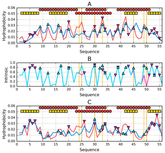
Figure 1.
Theoretical (T—blue) and observed (O—red) hydrophobicity profiles for (A)—2JWS and (C)—2JWU. (B)—intrinsic hydrophobicity (H) profiles for: 2JWS—cyan and 2JWU—magenta. Two rows of markers at the top of A and C denote locations of secondary structure motifs present in 2JWS (first row) and 2JWU (second row): red circles—α-helices, yellow squares—β-sheets. Triangle markers on A, B and C distinguish residues involved in the construction of hydrophobic nucleus: 2JWS—cyan/pointing up, 2JWU—magenta/pointing down. Vertical orange lines go through locations where sequences of the compared proteins differ.
There are 7 mutational changes in the compared proteins, but from the point of view of the structure of the hydrophobic nucleus, only the conversion of Leu (2JWS) to Lys (2JWU) at position 50 and the change accompanying it at position 49 (49Thr in 2JWU and 49Ile in 2JWS) are relevant. Together, the change in this location significantly increases the level of hydrophobicity in 2JWS. Other changes due to the marginal small difference do not seem to matter.
The status of proteins in the light of the fuzzy oil drop model expressed by the RD parameter is 0.335 for 2JWU and 0.370 for 2JWS. In both cases, therefore, the protein contains an ordered hydrophobic core with a high concentration of hydrophobicity at the centre of the molecule along with a polar mantle on the surface. The respective profiles for T and O hydrophobicity in both proteins in question are shown in Figure 1A,C.
The slightly higher RD value for 2JWS results from the status of chain fragment 22–37, where the difference between the distribution of T and O is visible. In this chain fragment two mutated residues are present.
The sections that make up the components of the hydrophobic core have been marked with circles, and the surface sections with the low—as expected—level of hydrophobicity are marked with rectangles.
The determined sections included in the hydrophobic core were distinguished on the presentation of the 3D structure (Figure 2).
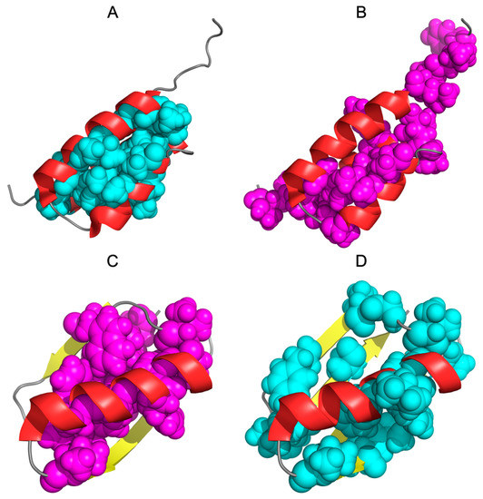
Figure 2.
Three-dimensional presentation of 2JWS and 2JWU: (A)—2JWS with teal spheres highlighting the hydrophobic core according to the hydrophobicity distributions in this protein (corresponding to teal triangles on Figure 1). (B)—2JWS with magenta spheres highlighting the hydrophobic core according to the hydrophobicity distributions in 2JWU (corresponding to magenta triangles on Figure 1). (C)—2JWU with magenta spheres highlighting the hydrophobic core according to the hydrophobicity distributions in this protein (corresponding to magenta triangles on Figure 1). (D)—2JWU with cyan spheres highlighting the hydrophobic core according to the hydrophobicity distributions in 2JWS (corresponding to cyan triangles on Figure 1).
The structures presented in Figure 2A,B visualize the composition of the hydrophobic core determined for a given molecule. In contrast, the structures of Figure 2C,D show the location of residues that in the partner structure are part of the nucleus. This comparison reveals a different organization and commitment of different sections to the structure of the hydrophobic nucleus.
Figure 2B illustrates the final relationship—hydrophobic core structure—in the representation of intrinsic hydrophobicity distribution. Appropriately highlighted sections indicate two alternative systems of residues involved in the construction of a hydrophobic nucleus.
Two different scenarios for carrying out the task of “hydrophobic nucleus construction” are shown in Figure 3A, where the T distributions in both compared proteins were compared, and Figure 3B, where the O distributions in both proteins were compared.
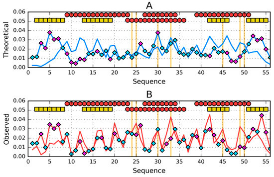
Figure 3.
Comparison of (A)—theoretical (T) and (B)—observed (O) hydrophobicity profiles for 2JWS and 2JWU (profiles for 2JWU have diamond markers on them). Two rows of markers at the top of A and B denote locations of secondary structure motifs present in 2JWS (first row) and 2JWU (second row): red circles—α-helices, yellow squares—β-sheets. Cyan diamond markers distinguish residues for which the difference between theoretical (on A) or observed (on B) distributions is lower than average. Magenta diamond markers do the opposite—show where this difference is above average. Vertical orange lines go through locations where sequences of the compared proteins differ.
Comparison of the T distributions for both structures reveals a central chain fragment with a very similar distribution. This chain fragment coincides with the location of the helix in both compared structures. Other fragments: N- and C-terminal show significant distribution differences.
A comparative analysis of O distributions reveals very similar differences. There is a high degree of similarity in the central part and significant differences in N- and C-terminal views.
The quantitative status of these sections is given in Table 2.
Table 2.
RD values for selected sections: secondary structure and three zones 1–25, 26–35 and 36–56 resulting from the presence of an everywhere occurring helix (in the area 26–35) with a high degree of agreement of the O distribution against the T distribution in each case. H—helix, B—β-strand, RC—random coil.
Residues highlighted in Figure 4 were identified based on the value of differences between the compared distributions. Comparison of the fragments in Figure 4 reveals the location of amino acids showing similar status in the two compared proteins. The ranges highlighted with frames were obtained by eliminating those items that increase the correlation coefficient until the value 0.758 for the distribution O and 0.622 for the distribution T.
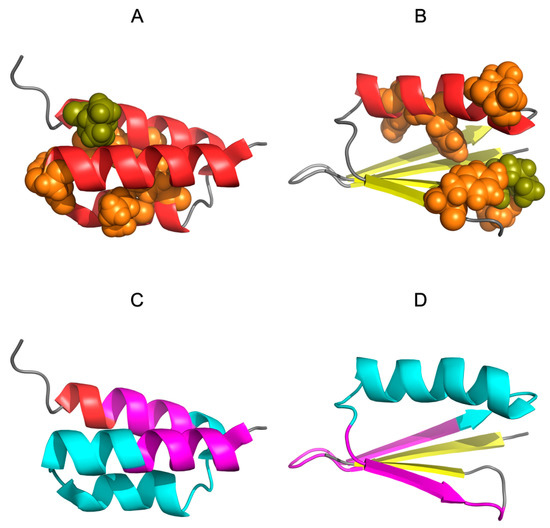
Figure 4.
Three-dimensional presentation of (A,C)—2JWS and (B,D)—2JWU. Orange spheres on A and B denote the mutations, among which—shown in olive—is Lys 50. Cyan fragment on C and D correspond to range 18–40 where the difference between theoretical distributions of 2JWS and 2JWU is low. Magenta fragments complement it to mark the range 8–48 where there is an accordance between observed distributions of these two proteins.
Figure 4 explains the reason for structural differences, which is position 50, where the hydrophobicity status was changed radically by replacing Leu (2JWS) with Lys (2JWU). This significant change as seen in Figure 4A,B is the reason for the completely different status of the chain fragment in the immediate vicinity of position 50. In 2JWS, Leu (and Ile in pos. 49) participates in the structure of the hydrophobic core, while in 2JWU, Lys in the same positions (50 and Thr at position 49) is exposed to the outside and participates in the construction of the outer mantle.
As can be seen in Figure 1B, all changes have a common direction—everywhere in 2JWS, the introduced change causes an increase in hydrophobicity in 2JWU or introduces a minimal reduction in hydrophobicity. Both structural forms show high compatibility of the T and O distribution, although the construction of a hydrophobic core with a higher concentration of hydrophobic residues results in a lower RD value for 2JWU. Increasing the proportion of residues with a higher level of hydrophobicity results in the presence of a more ordered hydrophobic core. In addition, the 2JWU structure also involves polypeptide chain fragment 1–7, which in 2JWS seems to be useless from the point of view of involvement in the construction of a hydrophobic core.
It should be noted that a significant change in the helical form to β-structured in the N-terminal section takes place in the fragment much preceding the location of the first mutation. The resulting conclusion indicates that the different organization of the N-terminal chain fragment has no direct cause in the mutation as such but is the result of a change present in the C-terminal fragment. It can be concluded that the final structure is a synergy effect in which the whole chain participates simultaneously.
3.2. Highly Homologous Sequences—Different Three-Dimensional Structures
A similar situation occurs in the case of highly homologous proteins with two structural forms showing a very similar arrangement: one of these forms is a completely helical protein—1ZXG—, and the other (similar to 2JWU) has a β-plate—1ZXH (similar to 2JWS)—in addition to the helical chain fragment. In addition, significant structural similarity of proteins is observed in pairs 1ZXG, 2JWU and 1ZXH, 2JWS.
A comparison of the T and O distributions for 1ZXG and 1ZXH expressed using RD (0.248 and 0.310, respectively) shows a very high compatibility of the hydrophobicity distribution in these proteins with the distribution idealized in both structural forms of these proteins.
Summaries of the profiles, Figure 1A, C and Figure 5A,C, reveal a high degree of similarity of distribution in proteins with significantly different sequences. Similarly to 2JWU, 1ZXH involves N- and C-terminal fragments for nuclear structure, while in 2JWS and 1ZXG, nuclear structure involves the central portion of the polypeptide chain. The similarity of the fragments is also characteristic, which in all discussed proteins take on a helical form.
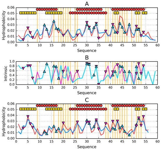
Figure 5.
Theoretical (T—blue) and observed (O—red) hydrophobicity profiles for (A)—1ZXG and (C)—1ZXH. (B)—intrinsic hydrophobicity (H) profiles for: 1ZXG—cyan and 1ZXH—magenta. Two rows of markers at the top of A and C denote locations of secondary structure motifs present in 1ZXG (first row) and 1ZXH (second row): red circles—α-helices, yellow squares—β-sheets. Triangle markers on A, B and C distinguish residues involved in the construction of hydrophobic core: 1ZXG—cyan/pointing up, 1ZXH—magenta/pointing down. Vertical orange lines go through locations where sequences of the compared proteins differ.
To underline the much higher degree of differentiation of intrinsic hydrophobicity, the summary is shown in Figure 5B.
The spatial structure reveals the specific position of residue 50. In both cases discussed here, Lys is in this position, so in both cases the residue is exposed. Figure 6 reveals a modelled arrangement of Lys50 within the helix in the exposure position, while this change of position 50 in 2JWU and 2JWS dramatically affected the structure of the immediate environment.
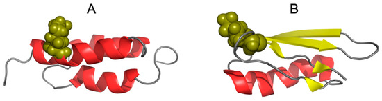
Figure 6.
Three-dimensional presentation of (A)—1ZXG and (B)—1ZXH. Olive spheres mark the location of Lys 50 in each protein.
In the case of 1ZXH and 1ZXG, the overall effect of sequence variability—or rather the distribution of hydrophobicity—finally leads to a different spatial form. Mutational changes result in a change in the periodicity of the hydrophobicity level. The 1:1 system preferring the β-form and the 1:2 or 2:1 system (proportions of hydrophilic to hydrophobic residues) supports the formation of a helical or β-form in proteins of such a small size, where almost all parts of the chain are in contact with the hydrophobic core (they participate in its generation) as well as the construction of the surface coating. In this situation, the helix should be hydropathic and the β-structure should represent a different character on both sides of the backbone line.
By interpreting the results given in Figure 7, a situation very similar to the previous example can be identified, where the central part of the polypeptide chain (marked as turquoise) forming the helical fragment shows great agreement in both O and T distribution. The differences are located in N- and C-terminal fragments.
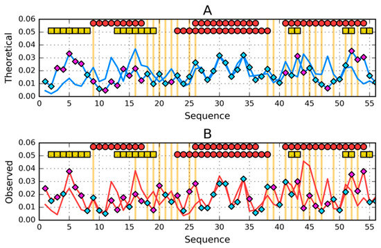
Figure 7.
Comparison of (A)—theoretical (T) and (B)—observed (O) hydrophobicity profiles for 1ZXG and 1ZXH (profiles for 1ZXH have diamond markers on them). Two rows of markers at the top of A and B denote locations of secondary structure motifs present in 1ZXG (first row) and 1ZXH (second row): red circles—α-helices, yellow squares—β-sheets. Cyan diamond markers distinguish residues for which the difference between theoretical (on A) or observed (on B) distributions is lower than average. Magenta diamond markers do the opposite—show where this difference is above average. Vertical orange lines go through locations where sequences of the compared proteins differ.
The number of mutations in this example is much higher than in the previous example (Figure 7). Therefore, it is difficult to clearly indicate one residue as responsible for structural differences. T distributions indicate the central fragment without mutations as representing very highly consistent distributions. Mutations mainly concern sections below position 30 and above position 38. In these sections differences in the distribution of T and O are identified.
Comparative analysis of the O distributions reveals similar characteristics (Figure 8B), where the heliacal fragment (central chain fragment) shows high similarity in both compared chains.
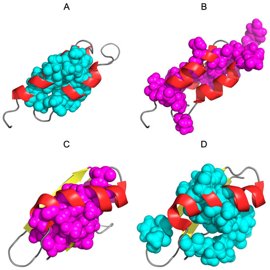
Figure 8.
Three-dimensional presentation of 1ZXG and 1ZXH: (A)—1ZXG with teal spheres highlighting the hydrophobic core according to the hydrophobicity distributions in this protein (corresponding to teal triangles on Figure 1). (B)—1ZXG with magenta spheres highlighting the hydrophobic core according to the hydrophobicity distributions in 1ZXH (corresponding to magenta triangles on Figure 1). (C)—1ZXH with magenta spheres highlighting the hydrophobic core according to the hydrophobicity distributions in this protein (corresponding to magenta triangles on Figure 1). (D)—1ZXH with cyan spheres highlighting the hydrophobic core according to the hydrophobicity distributions in 1ZXG (corresponding to cyan triangles on Figure 1).
Generally, a mutational change significantly increases the level of self-hydrophobicity of amino acids in the 1ZXH chain. The difference is about 8% in relation to the total value of 1ZXH self-hydrophobicity.
3.3. Comparative Cross-Analysis
The presence of 3D similarity between the 2JWU and 1ZXG proteins as well as the 2JWS and 1ZXH pairs suggests the possibility of cross-comparative analysis. It should be noted that the visible differences in the profiles below are identified at a very high degree of hydrophobic core structure reproduction expressed by RD values in all four proteins.
The summary of the total hydrophobicity of the analysed proteins is as follows:
24.97, 25.66, 26.78 and 27.83 for proteins 2JWU, 1ZXG, 2JWS and 1ZXG respectively. The total values for these proteins are comparable.
The list of changes in the amino acid sequence expressed by intrinsic hydrophobicity is illustrated in Figure 9A for the 1ZXG and 2JWS pair (both helical forms).
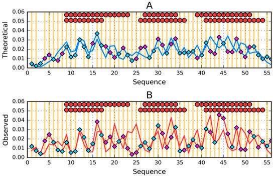
Figure 9.
Comparison of (A)—theoretical (T) and (B)—observed (O) hydrophobicity profiles for 2JWS and 1ZXG (profiles for 1ZXG have diamond markers on them). Two rows of markers at the top of A and B denote locations of secondary structure motifs present in 2JWS (first row) and 1ZXG (second row): red circles—α-helices, yellow squares—β-sheets (absent here). Cyan diamond markers distinguish residues for which the difference between theoretical (on A) or observed (on B) distributions is lower than average. Magenta diamond markers do the opposite—show where this difference is above average. Vertical orange lines go through locations where sequences of the compared proteins differ.
Analysis of T and O profiles (Figure 9A,B) shows very high similarity over the entire length of the chain with significantly different intrinsic hydrophobicity characteristics (Figure 9A).
The profiles also show sections that in the form of 1ZXH and 2JWU have β-structural status.
The second pair of 1ZXH and 2JWU, similarly to the previous pair, shows high similarity of both T and O profiles (Figure 10A,B) despite visible significant differences in intrinsic hydrophobicity (Figure 10A). The interpretation is very similar to the one given for the 1ZXG and 2JWS sets.
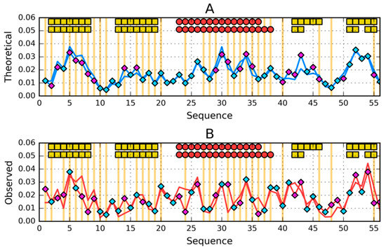
Figure 10.
Comparison of (A)—theoretical (T) and (B)—observed (O) hydrophobicity profiles for 2JWU and 1ZXH (profiles for 1ZXH have diamond markers on them). Two rows of markers at the top of A and B denote locations of secondary structure motifs present in 2JWU (first row) and 1ZXH (second row): red circles—α-helices, yellow squares—β-sheets (absent here). Cyan diamond markers distinguish residues for which the difference between theoretical (on A) or observed (on B) distributions is lower than average. Magenta diamond markers do the opposite—show where this difference is above average. Vertical orange lines go through locations where sequences of the compared proteins differ.
The quantitative assessment of the status of compared proteins and sections with a specific secondary structure is given in Table 2. RD values get (except for polypeptide chain fragment 42–48 in 2JWU) very low values everywhere, which confirms the high compliance of T and O distributions in the discussed proteins. The centrally located helical fragment shows an extremely high fit in all the forms discussed.
The central section is noteworthy (referred to as 26–35), which has a very low RD value in all forms.
3.4. Status of Sections with a Specific Secondary Structure
The participation in the hydrophobic core formation of fragments with a specific secondary structure and sections 1–25, 26–35 and 36–56 resulted from the location of the helical fragment with high compliance on the RD scale and was observed in all analysed structures.
Characteristics of the degree of sequence similarity expressed by correlation coefficient values for intrinsic hydrophobicity, for obvious reasons, are very high for the 2JWU and 2JWS pair and for the 1ZXH and 1ZXG pair, especially for the helical fragment of the chains (Table 3). The very low correlation coefficient for the 1ZXG and 2JWS relations for the N-terminal and C-terminal fragment is surprising. Despite this, these episodes take a similar helical form, which is not surprising in the case of the 2JWU and 1ZXG pair with a different secondary structure. Other correlation coefficient values for the remaining relationships reveal the degree of relationship between the similarity of structure and sequence determined by intrinsic hydrophobicity. The high (highest in all cases) correlation coefficient for the helix, which is present in all compared proteins in the same location, is noteworthy.
Table 3.
Correlation coefficients of intrinsic (HvH), observed (OvO) and theoretical (TvT) distributions for fragments 1–25, 26–35 and 35–56 from discussed proteins.
The degree of structural similarity was also assessed using the Dali program [65]. The degree of similarity expressed using RMS-D—root mean square for distance change for the pair of proteins 2JWU and 1ZXH is 1.9 A and for the 2JWS and 1ZXG RMS-D pair is 4.3 A. This shows a high degree of similarity in the 3D structure of the compared proteins.
3.5. Comparison of the Structural Code List
A more specific secondary structure variation is needed for full comparative analysis. It is expressed here using so-called structural codes, which are described in detail in [57,58,59,60]. It should be noted here that the C code corresponds to the helical form and the E code represents the β-structured form. The D code, on the other hand, is the transition zone between the helical C and β-structural E. The F code represents the status of the residue that ends the β-structural fragment. The G code is a left-handed helix. Analysis of the distribution of Phi and Psi angles, taking into account the division into zones determined on the basis of backbone conformation preferences, shows the location of changes in these zones in the compared proteins.
The location of the zones (codes A–G) and the representation of these zones in these proteins is shown in Figure 11.
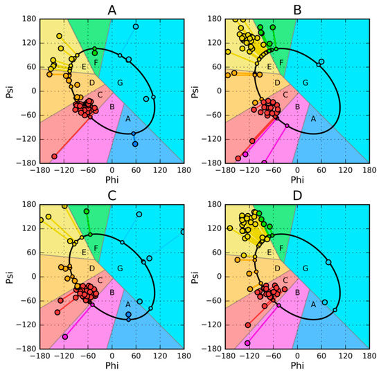
Figure 11.
Phi, Psi scatter plots and determination of structural codes for discussed proteins: (A)—2JWS, (B)—2WJU, (C)—1ZXG, (D)—1ZXH. Each residue is represented by a large circle marker and a small circle marker—its projection onto the ellipse, joined together by a line.
Map analysis (Figure 11) reveals the diversity of Phi and Psi angle distribution in the discussed proteins, including the zones defining structural codes. The use of codes reveals changes in the status of individual amino acids in the chain, as shown in Figure 12.
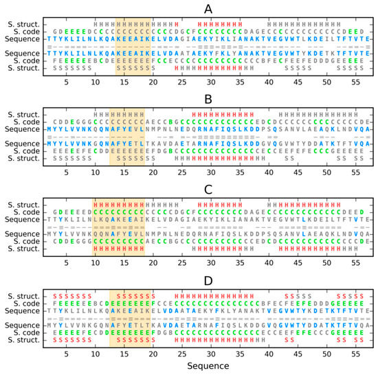
Figure 12.
Comparison of sequences, structural codes and secondary structure motifs of discussed proteins: (A)—2JWS vs. 2JWU, (B)—1ZXG vs. 1ZXG, (C)—2JWS vs. 1ZXG, (D)—2JWU vs. 1ZXH (first protein above, second below the central line). Matches in sequences are shown in blue, in structural codes in green, in secondary structure in red (H—helix, S—sheet), and mismatches are grey. Number of dashes in the central line denotes number of matches (3–0). Orange backgrounds distinguish the location of continuous change of structural codes on A and B and equality of structural codes on C and D.
The analysis of Figure 11 and Figure 12 reveals structural changes in the presentation covering the whole molecule. Sections of the common helix present in all of these proteins are visible. There are also chain fragments that in their respective pairs changed their status from helix (C) to β-structure (E). Zone D—the zone located between the helix area and β-structure—is particularly important because the conformational change between the helix and β-structure must occur through zone D. The proximity of residues representing the structural code D is observed in forms with the current β-structure in place of the helix. These items appear in the chain fragments preceding the β-structural fragments. The changes in Ile-Phe and Ile-Tyr in the 2JWS and 2JWU proteins do not seem to affect structural differentiation, all the more so that considering the spatial presentation, these residues are hydrophobic core participants regardless of the secondary structure (Figure 2). On the other hand, the sequence structure in the C-terminal fragment of the 1ZXH and 1ZXG proteins appears to have a significant impact on the secondary structure, where the involvement of the E form in 1ZXH appears to be the result of mutational changes. The sequence change affected the secondary form, but as in the previous case, it does not affect the share of this fragment in the structure of the hydrophobic core as shown in the analysis based on the fuzzy oil drop model in the first part of this work. Another observation is the significant sequence similarity in the C-terminal sections 2JWU and 1ZXH, where in both forms the β-structure is present (code E).
A completely similar situation occurs with the cro proteins pair 2PIJ and 3BD1, the signal transduction proteins 3CHY and electron transfer 1RCF (not shown here).
4. Discussion
The discussed set of proteins and the applied computational technique based on the fuzzy oil drop model and structural codes illustrating the changes in the secondary structure reveal the diverse organization of the structure of the hydrophobic core. The most important thing is that regardless of the secondary form, the overarching tendency in all of these proteins is the desire to generate a hydrophobic core. In these proteins the dominant importance of generating nuclear structure (understood along with the structure of the outer shell) has been demonstrated. Together, these two states produce the structure preferred by the aquatic environment, regardless of the secondary form.
The analysis presented here is important for identifying organizational change in the case of amyloids. Two available proteins in both their native and amyloid forms revealed different synergies in the organization of the core in these two structural forms with unchanged sequence [66]. These changes occur without any mutational change. Examples of proteins closely matching this situation are the 2JWU and 2JWS proteins, where the minimum number of changes results in a rather radical structural effect.
The goal of ensuring the presence of a hydrophobic core was achieved in all proteins during the folding process of these proteins, which is indicated by very low values of the RD parameter. However, the presence of the core was achieved by using different sections of the polypeptide chain. While proteins with the current β-plate N- and C-terminal sections clearly participate in the structure of the core, in the case of completely helical proteins, the core is built with the participation of sections from the central part of the chain. The high degree of sequence similarity in 2JWS and 2JWU (87.5% identity of residues) indicates, with a minimized number of factors affecting the change in structure, the important role of the presence of Leu and Lys at position 50. This residue seems to direct the process towards Leu’s participation in generating the core while Lys obtained a position exposed on the surface of the protein.
The relation of the number of identical residues in sections with a different secondary structure is important.
A single mutation may not have any impact on the final structure, but also—depending on the environment—may be critical for obtaining a native structure. Therefore, the conclusion of this work is the common phenomenon of the pursuit of a folding protein to generate a hydrophobic core aimed at isolating hydrophobic residues from the aquatic environment. How is this goal achieved? It depends on the type of synergy and thus some specific interaction of many residues that are able to generate a spatial form or in the form of a spherical micelle collectively—and this is implemented by globular proteins. Figure 1 shows a different way of achieving the common goal of generating a hydrophobic core. Some proteins unable to obtain the spherical micelle structure (globular proteins) shape the tape form from a centrally—but in the form of an elongated band—located hydrophobic core corresponding to the tape micelle. In this way, a band micelle is obtained, which is generated by amyloid proteins. Amyloids represent a structural form with a hydrophobic core in the form of a tape running along the long axis of fibril surrounding it with better or worse matched bands with low hydrophobicity [48,49,50,51,52]. Thus, amyloids are a synergy that is different from the native form, leading to an alternative solution to the impact and presence of a polar aquatic environment.
An example of reaching the structurally different forms 3α and 4β + α of proteins caused solely by one mutation is the perfect object for discussion in the field of sequence-to-structure relation [67]. The structures described in [67] will be taken under consideration to assess the hydrophobic core status using the fuzzy oil drop model as criterion.
5. Conclusions
Two proteins with very low sequence difference (3 residues in chain of 56 aa) with different secondary structures expressed by helical form changed to β-structure for fragments 10–20 and 40–50 are taken as examples to show the influence of hydrophobic core formation on native structure formation. Both proteins represent structures of high accordance between an idealized hydrophobicity distribution and an observed one. It also proves the important participation of the hydrophobic core in the synergy directing folding process toward hydrophobic core formation and consequently toward native form formation. This observation is supported by two other proteins with lower sequence similarity.
Author Contributions
Conceptualization, I.R. and L.K.; methodology, I.R.; software, M.B. and P.F.; validation, K.S. and I.R.; formal analysis, I.R.; investigation, K.S.; resources, K.S.; data curation, M.P.-K.; writing—original draft preparation, I.R. and K.S.; writing—review and editing, I.R.; visualization, M.B.; supervision, L.K.; project administration, I.R.; funding acquisition, I.R. and M.B. All authors have read and agreed to the published version of the manuscript.
Funding
This research was funded by Jagiellonian University—Medical College, grant numbers N41/DBS/000211, N41/DBS/000208.
Acknowledgments
We are indebted to Anna Śmietańska and Zdzisław Wiśniowski for technical support.
Conflicts of Interest
The authors declare no conflicts of interest.
References
- Dill, K.A.; MacCallum, J.L. The Protein-Folding Problem, 50 Years On. Science 2012, 338, 1042–1046. [Google Scholar] [CrossRef]
- Levinthal, C. Are there pathways for protein folding? J. Chim. Phys. 1968, 65, 44–45. [Google Scholar] [CrossRef]
- Levinthal, C. How to Fold Graciously. Mossbauer Spectroscopy in Biological Systems. In Proceedings of the Meeting Held at Allerton House, Monticello, IL, USA, 17–18 March 1969; University of Illinois Press: Urbana, IL, USA, 1969; Volume 67, pp. 22–24. [Google Scholar]
- Zwanzig, R.; Szabo, A.; Bagchi, B. Levinthal’s paradox. Proc. Natl. Acad. Sci. USA 1992, 89, 20–22. [Google Scholar] [CrossRef]
- Dill, K.A.; Chan, H.S. From Levinthal to pathways to funnels. Nat. Struct. Mol. Biol. 1997, 4, 10–19. [Google Scholar] [CrossRef]
- Karplus, M. The Levinthal paradox: Yesterday and today. Fold. Des. 1997, 2, S69–S75. [Google Scholar] [CrossRef]
- Durup, J. On “Levinthal paradox” and the theory of protein folding. J. Mol. Struct. THEOCHEM 1998, 424, 157–169. [Google Scholar] [CrossRef]
- Anfinsen, C.B. Principles that Govern the Folding of Protein Chains. Science 1973, 181, 223–230. [Google Scholar] [CrossRef] [PubMed]
- Anfinsen, C.B.; Scheraga, H.A. Experimental and Theoretical Aspects of Protein Folding. Adv. Protein Chem. 1975, 29, 205–300. [Google Scholar] [CrossRef] [PubMed]
- Bai, Y. Hidden intermediates and levinthal paradox in the folding of small proteins. Biochem. Biophys. Res. Commun. 2003, 305, 785–788. [Google Scholar] [CrossRef]
- Chothia, C. Hydrophobic bonding and accessible surface area in proteins. Nature 1974, 248, 338–339. [Google Scholar] [CrossRef]
- Tanford, C. The hydrophobic effect and the organization of living matter. Science 1978, 200, 1012–1018. [Google Scholar] [CrossRef] [PubMed]
- Tanford, C. Interfacial free energy and the hydrophobic effect. Proc. Natl. Acad. Sci. USA 1979, 76, 4175–4176. [Google Scholar] [CrossRef] [PubMed]
- Kauzmann, W. Structural factors in protein denaturation. J. Cell. Physiol. Suppl. 1956, 47 (Suppl. 1), 113–131. [Google Scholar] [CrossRef] [PubMed]
- Kauzmann, W. Some Factors in the Interpretation of Protein Denaturation. Adv. Protein Chem. 1959, 14, 1–63. [Google Scholar] [CrossRef]
- Chandler, D. Interfaces and the driving force of hydrophobic assembly. Nature 2005, 437, 640–647. [Google Scholar] [CrossRef]
- Tanford, C. My debt to Walter Kauzmann. Biophys. Chem. 2003, 105, 159–160. [Google Scholar] [CrossRef]
- Ripoll, D.R.; Piela, L.; Váasquez, M.; Scheraga, H.A. On the multiple-minima problem in the conformational analysis of polypeptides. V. Application of the self-consistent electrostatic field and the electrostatically driven monte carlo methods to bovine pancreatic trypsin inhibitor. Proteins Struct. Funct. Genet. 1991, 10, 188–198. [Google Scholar] [CrossRef]
- Kryshtafovych, A.; Monastyrskyy, B.; Fidelis, K.; Moult, J.; Schwede, T.; Tramontano, A. Evaluation of the template-based modeling in CASP12. Proteins Struct. Funct. Bioinform. 2017, 86, 321–334. [Google Scholar] [CrossRef]
- Osguthorpe, D. Ab initio protein folding. Curr. Opin. Struct. Biol. 2000, 10, 146–152. [Google Scholar] [CrossRef]
- Available online: http://predictioncenter.org (accessed on 25 January 2020).
- Elofsson, A.; Joo, K.; Keasar, C.; Lee, J.; Maghrabi, A.H.A.; Manavalan, B.; McGuffin, L.J.; Hurtado, D.M.; Mirabello, C.; Pilstål, R.; et al. Methods for estimation of model accuracy in CASP12. Proteins Struct. Funct. Bioinform. 2017, 86, 361–373. [Google Scholar] [CrossRef]
- Kryshtafovych, A.; Monastyrskyy, B.; Fidelis, K.; Schwede, T.; Tramontano, A. Assessment of model accuracy estimations in CASP12. Proteins Struct. Funct. Bioinform. 2017, 86, 345–360. [Google Scholar] [CrossRef] [PubMed]
- Keasar, C.; McGuffin, L.J.; Wallner, B.; Chopra, G.; Adhikari, B.; Bhattacharya, D.; Blake, L.; Bortot, L.O.; Cao, R.; Dhanasekaran, B.K.; et al. An analysis and evaluation of the WeFold collaborative for protein structure prediction and its pipelines in CASP11 and CASP12. Sci. Rep. 2018, 8, 9939. [Google Scholar] [CrossRef] [PubMed]
- Khoury, G.A.; Liwo, A.; Khatib, F.; Zhou, H.; Chopra, G.; Bacardit, J.; Bortot, L.O.; Faccioli, R.A.; Deng, X.; He, Y.; et al. WeFold: A coopetition for protein structure prediction. Proteins Struct. Funct. Bioinform. 2014, 82, 1850–1868. [Google Scholar] [CrossRef]
- Gregersen, N.; Bross, P.; Vang, S.; Christensen, J.H. Protein Misfolding and Human Disease. Annu. Rev. Genom. Hum. Genet. 2006, 7, 103–124. [Google Scholar] [CrossRef] [PubMed]
- Tian, P.; Best, R.B. Structural Determinants of Misfolding in Multidomain Proteins. PLoS Comput. Biol. 2016, 12, e1004933. [Google Scholar] [CrossRef] [PubMed]
- Dobson, C.M. Principles of protein folding, misfolding and aggregation. Semin. Cell Dev. Biol. 2004, 15, 3–16. [Google Scholar] [CrossRef] [PubMed]
- Carbonell, F.; Iturria-Medina, Y.; Evans, A.C. Mathematical Modeling of Protein Misfolding Mechanisms in Neurological Diseases: A Historical Overview. Front. Neurol. 2018, 9, 37. [Google Scholar] [CrossRef]
- Serpell, L. Amyloid structure. Essays Biochem. 2014, 56, 1–10. [Google Scholar] [CrossRef]
- Al-Garawi, Z.S.; Morris, K.L.; Marshall, K.E.; Eichler, J.; Serpell, L.C. The diversity and utility of amyloid fibrils formed by short amyloidogenic peptides. Interface Focus 2017, 7, 20170027. [Google Scholar] [CrossRef]
- Chothia, C. Principles that Determine the Structure of Proteins. Annu. Rev. Biochem. 1984, 53, 537–572. [Google Scholar] [CrossRef]
- Creighton, T.E.; Chothia, C. Selecting buried residues. Nature 1989, 339, 14–15. [Google Scholar] [CrossRef] [PubMed]
- Miller, S.; Lesk, A.M.; Janin, J.; Chothia, C. The accessible surface area and stability of oligomeric proteins. Nature 1987, 328, 834–836. [Google Scholar] [CrossRef] [PubMed]
- Miller, S.; Janin, J.; Lesk, A.M.; Chothia, C. Interior and surface of monomeric proteins. J. Mol. Biol. 1987, 196, 641–656. [Google Scholar] [CrossRef]
- Dill, K.A.; Flory, P.J. Molecular organization in micelles and vesicles. Proc. Natl. Acad. Sci. USA 1981, 78, 676–680. [Google Scholar] [CrossRef] [PubMed]
- Sałapa, K.; Kalinowska, B.; Jadczyk, T.; Roterman, I. Measurement of Hydrophobicity Distribution in Proteins—Non-redundant Protein Data Bank. Bio-Algorithms Med.-Syst. 2012, 8, 327–338. [Google Scholar] [CrossRef]
- Kalinowska, B.; Banach, M.; Wiśniowski, Z.; Konieczny, L.; Roterman, I. Is the hydrophobic core a universal structural element in proteins? J. Mol. Mod. 2017, 23, 205. [Google Scholar] [CrossRef]
- Banach, M.; Konieczny, L.; Roterman-Konieczna, I. Ligand-binding-site recognition. In Protein Folding in Silico; Woodhead Publishing: Cambridge, UK, 2012; pp. 79–93. [Google Scholar] [CrossRef]
- Banach, M.; Konieczny, L.; Roterman-Konieczna, I. Can the Structure of the Hydrophobic Core Determine the Complexation Site. In Identification of Ligand Binding Site and Protein-Protein Interaction Area; Roterman-Konieczna, I., Ed.; Springer—Focus on Structural Biology: Berlin/Heidelberg, Germany, 2012; pp. 41–54. [Google Scholar] [CrossRef]
- Banach, M.; Konieczny, L.; Roterman-Konieczna, I. Use of the “fuzzy oil drop” model to identify the complexation area in protein homodimers. In Protein Folding in Silico; Roterman-Konieczna, I., Ed.; Woodhead Publishing: Cambridge, UK, 2012; pp. 95–122. [Google Scholar] [CrossRef]
- Lesk, A.M.; Chothia, C. Solvent accessibility, protein surfaces, and protein folding. Biophys. J. 1980, 32, 35–47. [Google Scholar] [CrossRef]
- Gerstein, M.; Chothia, C. Packing at the protein-water interface. Proc. Natl. Acad. Sci. USA 1996, 93, 10167–10172. [Google Scholar] [CrossRef]
- Chiche, L.; Gregoret, L.M.; Cohen, F.E.; Kollman, P.A. Protein model structure evaluation using the solvation free energy of folding. Proc. Natl. Acad. Sci. USA 1990, 87, 3240–3243. [Google Scholar] [CrossRef]
- Fisher, H.F. A limiting law relating the size and shape of protein molecules to their composition. Proc. Natl. Acad. Sci. USA 1964, 51, 1285–1291. [Google Scholar] [CrossRef]
- Tanford, C. How protein chemists learned about the hydrophobic factor. Protein Sci. 1997, 6, 1358–1366. [Google Scholar] [CrossRef] [PubMed]
- Konieczny, L.; Brylinski, M.; Roterman, I. Gauss-function-Based model of hydrophobicity density in proteins. Silico Biol. 2006, 6, 15–22. [Google Scholar]
- Kalinowska, B.; Banach, M.; Konieczny, L.; Roterman, I. Application of Divergence Entropy to Characterize the Structure of the Hydrophobic Core in DNA Interacting Proteins. Entropy 2015, 17, 1477–1507. [Google Scholar] [CrossRef]
- Fabian, P.; Stapor, K.; Banach, M.; Ptak-Kaczor, M.; Konieczny, L.; Roterman, I. Different Synergy in Amyloids and Biologically Active Forms of Proteins. Int. J. Mol. Sci. 2019, 20, 4436. [Google Scholar] [CrossRef] [PubMed]
- Dułak, D.; Gadzała, M.; Banach, M.; Ptak, M.; Wisniowski, Z.; Konieczny, L.; Roterman, I. Filamentous Aggregates of Tau Proteins Fulfil Standard Amyloid Criteria. Int. J. Mol. Sci. 2018, 19, 2910. [Google Scholar] [CrossRef] [PubMed]
- Roterman, I.; Dułak, D.; Gadzała, M.; Banach, M.; Konieczny, L. Structural analysis of the Aβ(11–42) amyloid fibril based on hydrophobicity distribution. J. Comput. Aided Mol. Des. 2019, 33, 665–675. [Google Scholar] [CrossRef] [PubMed]
- Dułak, D.; Banach, M.; Gadzała, M.; Konieczny, L.; Roterman, I. Structural analysis of the Aβ(15-40) amyloid fibril based on hydrophobicity distribution. Acta Biochim. Pol. 2018, 65, 595–604. [Google Scholar] [CrossRef]
- He, Y.; Chen, Y.; Alexander, P.; Bryan, P.; Orban, J. NMR structures of two designed proteins with 88% sequence identity but different fold and function. Proc. Natl. Acad. Sci. USA 2008, 105, 14412–14417. [Google Scholar] [CrossRef]
- He, Y.; Yeh, D.C.; Alexander, P.; Bryan, P.N.; Orban, J. Solution NMR Structures of IgG Binding Domains with Artificially Evolved High Levels of Sequence Identity but Different Folds. Biochemistry 2005, 44, 14055–14061. [Google Scholar] [CrossRef]
- Dawson, N.L.; Lewis, T.E.; Das, S.; Lees, J.G.; Lee, D.; Ashford, P.; Orengo, C.A.; Sillitoe, I. CATH: An expanded resource to predict protein function through structure and sequence. Nucleic Acids Res. 2016, 45, D289–D295. [Google Scholar] [CrossRef]
- Banach, M.; Kalinowska, B.; Konieczny, L.; Roterman, I. Structural Role of Hydrophobic Core in Proteins-Selected Examples. J. Proteom. Bioinform. 2016, 9, 276–286. [Google Scholar] [CrossRef]
- Jurkowski, W.; Baster, Z.; Dułak, D.; Roterman-Konieczna, I. The early-stage intermediate. In Protein Folding in Silico; Woodhead Publishing: Cambridge, UK, 2012; pp. 1–20. [Google Scholar] [CrossRef]
- Kalinowska, B.; Fabian, P.; Stąpor, K.; Roterman, I. Statistical dictionaries for hypothetical in silico model of the early-stage intermediate in protein folding. J. Comput. Aided Mol. Des. 2015, 29, 609–618. [Google Scholar] [CrossRef] [PubMed]
- Roterman, I. The geometrical analysis of peptide backbone structure and its local deformations. Biochimie 1995, 77, 204–216. [Google Scholar] [CrossRef]
- Roterman, I. Modelling the Optimal Simulation Path in the Peptide Chain Folding–Studies Based on Geometry of Alanine Heptapeptide. J. Theor. Biol. 1995, 177, 283–288. [Google Scholar] [CrossRef]
- Roterman, I.; Konieczny, L.; Jurkowski, W.; Prymula, K.; Banach, M. Two-intermediate model to characterize the structure of fast-folding proteins. J. Theor. Biol. 2011, 283, 60–70. [Google Scholar] [CrossRef]
- Levitt, M. A simplified representation of protein conformations for rapid simulation of protein folding. J. Mol. Biol. 1976, 104, 59–107. [Google Scholar] [CrossRef]
- Kullback, S.; Leibler, R.A. On Information and Sufficiency. Ann. Math. Stat. 1951, 22, 79–86. [Google Scholar] [CrossRef]
- Alexander, P.A.; He, Y.; Chen, Y.; Orban, J.; Bryan, P.N. The design and characterization of two proteins with 88% sequence identity but different structure and function. Proc. Natl. Acad. Sci. USA 2007, 104, 11963–11968. [Google Scholar] [CrossRef]
- De Beer, T.A.P.; Berka, K.; Thornton, J.M.; Laskowski, R.A. PDBsum additions. Nucleic Acids Res. 2013, 42, D292–D296. [Google Scholar] [CrossRef]
- Holm, L.; Rosenström, P. Dali server: Conservation mapping in 3D. Nucleic Acids Res. 2010, 38, W545–W549. [Google Scholar] [CrossRef]
- He, Y.; Chen, Y.; Alexander, P.A.; Bryan, P.N.; Orban, J. Mutational tipping points for switching protein folds and functions. Structure 2012, 20, 283–291. [Google Scholar] [CrossRef] [PubMed]


© 2020 by the authors. Licensee MDPI, Basel, Switzerland. This article is an open access article distributed under the terms and conditions of the Creative Commons Attribution (CC BY) license (http://creativecommons.org/licenses/by/4.0/).