Multi-Criteria Pythagorean Fuzzy Group Decision Approach Based on Social Network Analysis

Abstract

With the development of social media, the social relationships among group decision makers should be taken into consideration when addressing group decision making problems. As an extension of the fuzzy set, the Pythagorean fuzzy set has recently been applied to depict the uncertainty in practical group decision problems. The purpose of this paper is to propose a multi-criteria Pythagorean fuzzy group decision approach considering social relations. In this paper, the similarity degree and the paths between any two experts in a social network are combined to construct a connection strength matrix to detect the leader among all the experts. A leader-following consensus reaching algorithm is proposed to adjust the multi-criteria Pythagorean fuzzy decision making matrix. Moreover, a procedure for the multi-criteria Pythagorean fuzzy group decision approach based on social network analysis is proposed. We use an example to illustrate the feasibility and advantages of the proposed method.

1. Introduction

Multi-criteria decision making (MCDM) aims to choose the best alternative from a finite set of alternatives with multiple criteria. Considering the inherent vagueness of human preferences, as well as the fact that objects are fuzzy and uncertain, Bellman and Zadeh introduced the theory of fuzzy sets into MCDM problems. Yager [1] introduced the Pythagorean fuzzy set (PFS) to extend the fuzzy set. The PFS is denoted by the membership degree and the non-membership degree, and their sum of squares is less than or equal to 1.

There are numerous articles that apply the PFS to address (group) decision making problems [2,3,4,5,6,7,8,9,10,11,12,13,14,15,16,17,18,19,20,21]. Zhang and Xu [2] extended the technique for order preference using the similarity to the ideal solution (TOPSIS) method to deal with multiple criteria decision making with PFS. Ren et al. [4] solved the MCDM problems with Pythagorean fuzzy information by extending the interactive multi-criteria decision making (TODIM) approach. Zeng et al. [5] addressed Pythagorean fuzzy multiple-criteria decision making problems by combining the Pythagorean fuzzy ordered weighted average distance operator and the TOPSIS method. Zhang [6] developed a novel Pythagorean fuzzy QUALIFLEX (qualitative flexible multiple criteria method) method based on a closeness index to deal with hierarchical multi-criteria Pythagorean fuzzy decision making problems. Zhang [7] developed a new method based on similarity measures to address multiple criteria group decision making problems with Pythagorean fuzzy numbers. Garg [9] proposed confidence Pythagorean fuzzy weighted and ordered weighted operators to address group decision making problems. Liang and Xu [11] combined Pythagorean fuzzy sets (PFS) and hesitant fuzzy sets (HFS) to propose a new concept of hesitant Pythagorean fuzzy sets (HPFS). Liang et al. [12] used Pythagorean fuzzy geometric Bonferroni mean and weighted Pythagorean fuzzy geometric Bonferroni mean operators to fuse the information in the Pythagorean fuzzy multi-criteria group decision making problem. Wei [14] developed several Pythagorean fuzzy interaction aggregation operators, including the Pythagorean fuzzy interaction weighted average (PFIWA) operator and the Pythagorean fuzzy interaction weighted geometric (PFIWG) operator. Xue et al. [20] extended the linear programming technique for the multi-dimensional analysis of preference (LINMAP) method to address multi-criteria Pythagorean fuzzy group decision making problems. Zeng et al. [21] introduced a novel aggregation method for the Pythagorean fuzzy set to solve multiple attribute decision making problems.

When addressing group decision making problems, all decision makers are supported to work together toward the same goals in order to reach a common decision. Thus, all the individual decision makers should achieve a consensus to make the final decision. However, the existing research studies about the multi-criteria Pythagorean fuzzy group decision approach do not consider this factor. Moreover, with the development of social media and e-commerce, social network relations may affect the process and results of decision making. With the development of big data technology, some big data tools have been developed to analyze social network data, such as FOLLOWERWONK (followerwonk.com, tracks follower gains and losses comparing twitter accounts), KLOUT (khoros.com, collects data from various resources and identifies influence over social networks), and QUINTLY (www.quintly.com, tracks and compares the performance of social media marketing). The social network relations among a group of decision makers can be measured in a variety of ways, including factors such as family, friends, business dealings, communications, emails, and romantic ties. Additionally, the social network can be obtained by data mining techniques from social media. The existing research studies on the multi-criteria Pythagorean fuzzy group decision approach do not take the social relations among decision makers into consideration. Moreover, most of the qualitative and quantitative methods used in grouped fuzzy systems aim at equal weighting in the voting process between the group members. Additionally, there are few research studies on the role of leaders in the group decision making process. In order to solve the above problems, we propose a novel multi-criteria Pythagorean fuzzy group decision approach based on social network analysis. The social relations and consensus reaching process are both considered in this paper.

The rest of the paper is set out as follows. In Section 2, we review the Pythagorean fuzzy set and social network analysis. In Section 3, the leader-following consensus reaching method for Pythagorean fuzzy group decision making is proposed. In Section 4, we establish the procedure for the multi-criteria Pythagorean fuzzy group decision making approach based on social network analysis (SNA). In Section 5, one illustrative example is presented to illustrate the application of the proposed model. This paper is concluded in Section 6.

2. Preliminaries

In this section, we review some basic definitions and concepts regarding Pythagorean fuzzy sets and social network analysis.

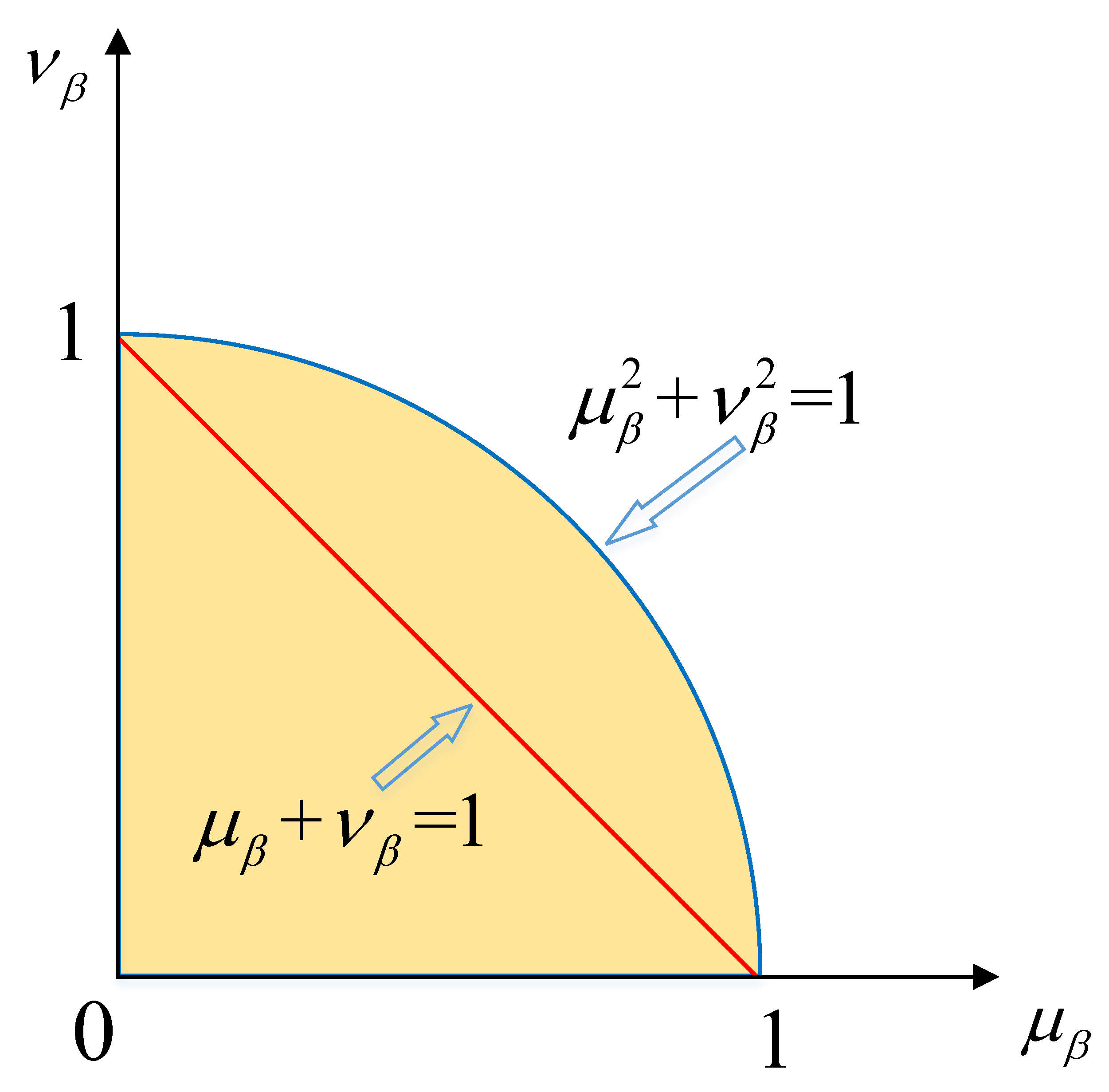
2.1. Pythagorean Fuzzy Set

Definition 1.

Let$X$ be an arbitrary non-empty set. A PFS is a mathematical object of the following form:

$$P=\left\{\langle x,P({\mu }_p(x),{\nu }_p(x))\rangle |x\in X\right\}$$

(1)

where ${\mu }_p(x),{\nu }_p(x):X\to \left[0,1\right]$, such that ${({\mu }_p(x))}^2+{({\nu }_p(x))}^2\le 1$, for every $x\in X$. Here, ${\mu }_p(x)$ and ${\nu }_p(x)$ denote the membership and non-membership degrees of the element $x$ to $X$ in $P$, respectively.

The hesitant degree of $x\in X$ is defined as:

$${\pi }_p(x)=\sqrt{1-{\mu }_P^2(x)-{\nu }_P^2(x)}$$

(2)

Here, $P({\mu }_P(x),{\nu }_P(x))$ is called the Pythagorean number (PFN), denoted by $\beta =P({\mu }_{\beta },{\nu }_{\beta })$, where ${\mu }_{\beta },{\nu }_{\beta }\in \left[0,1\right]$, ${\pi }_{\beta }=\sqrt{1-{({\mu }_{\beta })}^2-{({\nu }_{\beta })}^2}$, and ${({\mu }_{\beta })}^2+{({\nu }_{\beta })}^2\le 1$. The space of the PFN is shown in Figure 1.

In order to rank the PFNs, Wei [14] further gave a score function for the PFN:

Definition 2.

Let$\beta =P({\mu }_{\beta },{\nu }_{\beta })$be a PFN, then the score function of$\beta$ is defined as

$$SF(\beta )=\frac{1}{2}(1+{({\mu }_{\beta })}^2-{({\nu }_{\beta })}^2),SF(\beta )\in \left[0,1\right].$$

(3)

The larger the score, the better the PFN is.

Definition 3.

Let${\beta }_1$and${\beta }_2$be two PFNs, the distance between${\beta }_1$and${\beta }_2$is defined as follows:

$$d({\beta }_1,{\beta }_2)=\frac{1}{2}(|{({\mu }_{{\beta }_1})}^2-{({\mu }_{{\beta }_2})}^2|+|{({\nu }_{{\beta }_1})}^2-{({\nu }_{{\beta }_2})}^2|+|{({\pi }_{{\beta }_1})}^2-{({\pi }_{{\beta }_2})}^2|)$$

(4)

Definition 4.

Let${\beta }_j=P({\mu }_{{\beta }_j},{\nu }_{{\beta }_j})$($j=1,2,\dots ,n$) be a set of PFNs, then the Pythagorean fuzzy weighted averaging (PFWA) operator is defined as follows:

$$\begin{array}{ll}PFWA({\beta }_1,{\beta }_2,\dots ,{\beta }_n)& ={\xi }_1{\beta }_1\oplus {\xi }_2{\beta }_2\oplus \cdots \oplus {\xi }_n{\beta }_n\\ & =P(\sqrt{1-{\displaystyle \prod _{j=1}^N{(1-{({\mu }_{{\beta }_j})}^2)}^{{\xi }_j}}},{\displaystyle \prod _{j=1}^n{({\nu }_{{\beta }_j})}^{{\xi }_j}})\end{array}$$

(5)

where${\xi }_j$indicates the importance degree of${\beta }_j$, satisfying${\xi }_j\ge 0$($j=1,2,\dots ,n$) and${\displaystyle {\sum }_{j=1}^n{\xi }_j}=1$.

2.2. Social Network Analysis

Social network analysis (SNA) studies the relationships between social entities such as members of a group, corporations, or nations, and gives us a background that allows us, among other things, to examine the structural and locational properties, including centrality, prestige, and structural balance [22]. A network is made up of points, usually called nodes or vertices, along with the lines connecting them, usually called edges. A network can be mathematically represented by the adjacency matrix $A={\left[A_{ij}\right]}_{t\times t}$, where $A$ is a $t\times t$ symmetric matrix and $t$ is the number of vertices ($e_1,e_2,\cdots e_t$) [23]. The adjacency matrix has the following elements

$$A_{ij}=\{\begin{array}{ll}1& \mathrm{if}\mathrm{there}\mathrm{is}\mathrm{an}\mathrm{edge}\mathrm{between}\mathrm{vertices}{e}_i\mathrm{and}{e}_j\\ 0& \mathrm{otherwise}\end{array}$$

If there is an edge between $e_i$ and $e_j$, then there is also an edge between $e_j$ and $e_i$. Thus, the matrix is symmetric (i.e., $A_{ij}=A_{ji}$). It must be noted that we only focus on the completely connected undirected graph, where every pair of distinct vertices is connected by a unique edge in this paper.

In an undirected connected network, the distance between any two nodes is defined as follows.

Definition 5.

The distance$D(e_k,e_l)$between expert$e_k$and$e_l$($k,l=1,2,\dots ,t$) in an undirected connected network with$t$nodes is the shortest path between$e_k$and$e_l$. If there is more than one shortest path, the distance between two nodes is the length of any shortest path between them. According to the properties of the undirected connected network,$D(e_k,e_l)=D(e_l,e_k)$ remains constant.

For an undirected connected network with $t$ nodes, computing the distance between two nodes $e_k$ and $e_l$ ($k,l=1,2,\dots ,t$) can construct a distance matrix $D={\left[D_{kl}\right]}_{t\times t}={\left[D(e_k,e_l)\right]}_{t\times t}$. As such, $D(e_k,e_l)=D(e_l,e_k)$ remains constant, so the distance matrix $D$ is symmetrical. Notably, all elements on the main diagonal of $D$ are $0s$ because $D(e_k,e_k)=0$ always remains constant.

3. The Consensus Reaching Method for Pythagorean Fuzzy Group Decision Making

For consensus reaching process in a social network, the leader may influence the other individual experts, called followers. In this section, we study the followers to adjust their decision matrices according to the leader’s matrix in order to reach a consensus.

3.1. Problem Formulation

For the sake of convenience, the multi-criteria Pythagorean fuzzy group decision making problem in this paper is formulated as follows.

Let $X=\left\{x_1,x_2,\dots ,x_m\right\}$ ($m\ge 2$) be a collection of $m$ feasible alternatives, $C=\left\{C_1,C_2,\dots ,C_n\right\}$ be a set of criteria, and $W={(w_1,w_2,\dots ,w_n)}^T$ be the weight vector of the criteria, which satisfies $0\le w_j\le 1$ and ${\displaystyle {\sum }_{j=1}^n{w}_j}=1$. Let $E=\left\{e_1,e_2,\dots ,e_t\right\}$ be a group of experts with the adjacency matrix $A={\left[A_{ij}\right]}_{t\times t}$, and $\lambda =({\lambda }_1,{\lambda }_2,\dots ,{\lambda }_t)$ be the weight vector of the experts, where $0\le {\lambda }_k\le 1$ and ${\displaystyle {\sum }_{k=1}^t{\lambda }_k}=1$. Suppose that the expert $e_k$ evaluates the alternative $x_i$ ($i=1,2,\dots ,m$) with criterion $C_j$ ($j=1,2,\dots ,n$) by PFN $P({\mu }_{ij}^k,{\nu }_{ij}^k)$. Moreover, for the PFN $P({\mu }_{ij}^k,{\nu }_{ij}^k)$, ${\mu }_{ij}^k$ shows the degree to which the alternative $x_i$ satisfies the criterion $C_j$ and ${\nu }_{ij}^k$ shows the degree to which alternative $x_i$ dissatisfies the criterion $C_j$. Then, the decision matrix of the expert $e_k$ can be denoted as $P^k={\left[{\beta }_{ij}^k\right]}_{m\times n}={\left[P({\mu }_{ij}^k,{\nu }_{ij}^k)\right]}_{m\times n}$ ($k=1,2,\dots ,t$).

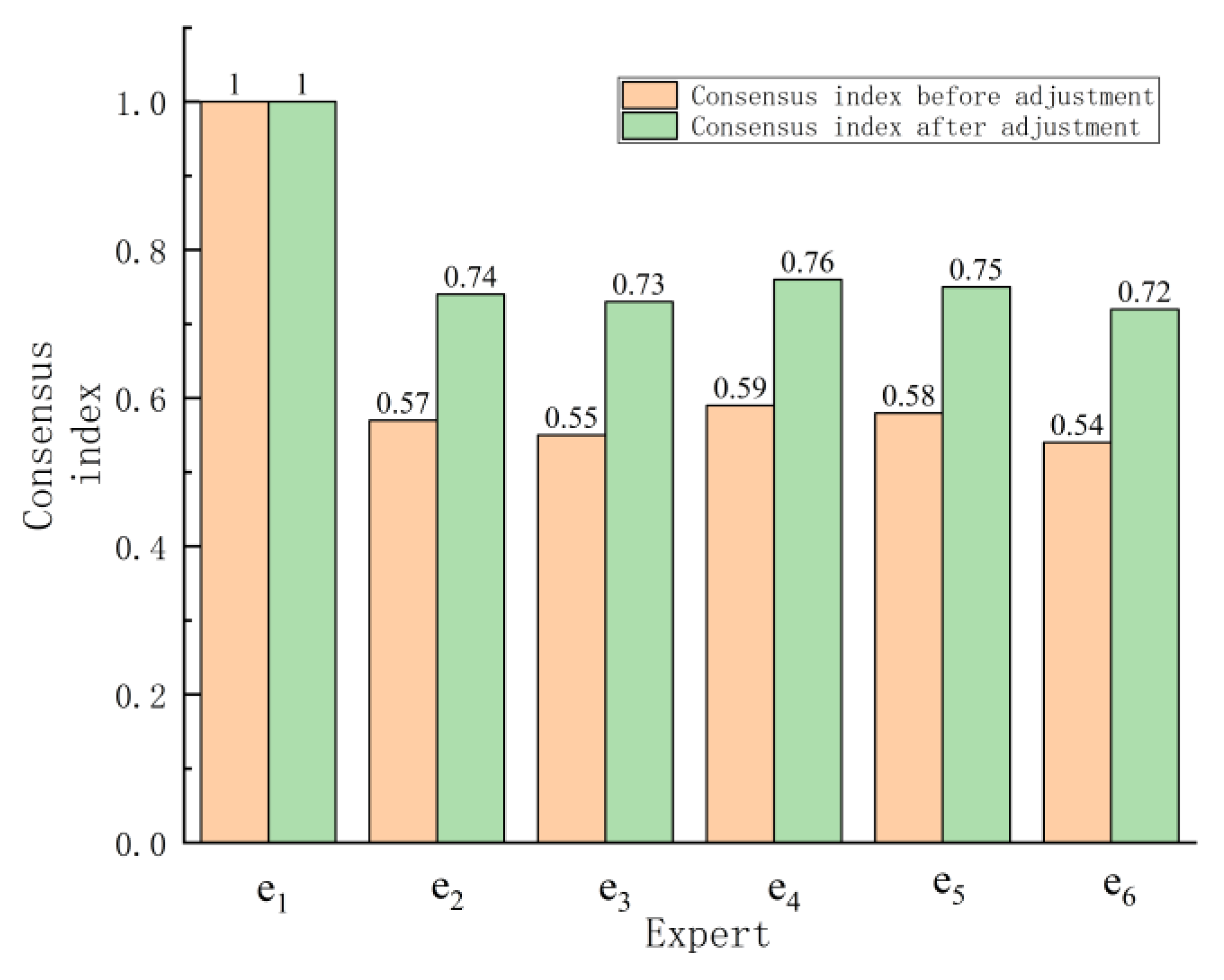
3.2. The Leader-Following Consensus Reaching Method

The similarity degree between any two experts can be calculated as follows.

Definition 6.

Let$e_k$and$e_l$be two experts with Pythagorean fuzzy group decision matrices$P^k={\left[{\beta }_{ij}^k\right]}_{m\times n}={\left[P({\mu }_{ij}^k,{\nu }_{ij}^k)\right]}_{m\times n}$and$P^l={\left[{\beta }_{ij}^l\right]}_{m\times n}={\left[P({\mu }_{ij}^l,{\nu }_{ij}^l)\right]}_{m\times n}$, respectively. The similarity degree$S(e_k,e_l)$between$e_k$and$e_l$ is defined as follows:

$$\begin{array}{ll}S(e_k,e_l)& \triangleq S(P^k,P^l)\\ & =\frac{1}{mn}{\displaystyle \sum _{i=1}^m{\displaystyle \sum _{j=1}^n(1-\frac{1}{2}(|{({\mu }_{ij}^k)}^2-{({\mu }_{ij}^l)}^2|+|{({\nu }_{ij}^k)}^2-{({\nu }_{ij}^l)}^2|+|{({\pi }_{ij}^k)}^2-{({\pi }_{ij}^l)}^2|))}}\end{array},k,l\in T$$

(6)

Theorem 1.

For experts$e_k$and$e_l$, whose similarity degrees are shown in Equation (6),$S(e_k,e_l)\in \left[0,1\right]$and$S(e_k,e_l)=S(e_l,e_k)$remain constant.

Proof of Theorem 1.

According to Equation (2), we have

$$\begin{array}{l}|{({\mu }_{ij}^k)}^2-{({\mu }_{ij}^l)}^2|+|{({\nu }_{ij}^k)}^2-{({\nu }_{ij}^l)}^2|+|{({\pi }_{ij}^k)}^2-{({\pi }_{ij}^l)}^2|\\ \le |{({\mu }_{ij}^k)}^2|+|{({\mu }_{ij}^l)}^2|+|{({\nu }_{ij}^k)}^2|+|{({\nu }_{ij}^l)}^2|+|{({\pi }_{ij}^k)}^2|+|{({\pi }_{ij}^l)}^2|.\\ =2\end{array}$$

Then, it follows that

$$0\le \frac{1}{2}(|{({\mu }_{ij}^k)}^2-{({\mu }_{ij}^l)}^2|+|{({\nu }_{ij}^k)}^2-{({\nu }_{ij}^l)}^2|+|{({\pi }_{ij}^k)}^2-{({\pi }_{ij}^l)}^2|)\le 1$$

Thus, $S(e_k,e_l)\in \left[0,1\right]$ can be obtained and $S(e_k,e_l)=S(e_l,e_k)$ can be easily proven. □

In this paper, we define $S={\left[S_{kl}\right]}_{t\times t}$ as the similarity matrix of all the experts where $S_{kl}=S(e_k,e_l)$. For any two directly connected experts in a social network, the similarity degree can be taken as the direct connection strength. Therefore, the undirected social network becomes a weighted one, and the corresponding adjacency matrix is denoted by $\stackrel{\prime }{A}$, where

$${\stackrel{\prime }{A}}_{kl}=\{\begin{array}{ll}{S}_{kl},& A_{kl}=1\\ 0,& A_{kl}=0\end{array}$$

(7)

Moreover, we can obtain $\stackrel{\prime }{A}$ by $\stackrel{\prime }{A}=A.*S$, where the operator $.*$ is the Hadamard multiplication of the matrix.

For the two experts who are indirectly connected in a social network, we can use the Einstein product to evaluate their connection strength [24].

Definition 7.

Let$e_k$and$e_l$ be two indirectly connected experts is a social network, where the shortest path from $e_k$ to $e_l$ is $e_k\to e_{x_1}\to e_{x_2}\to \cdots \to e_{x_{n-1}}\to e_l$. The connection strengths for $e_k\to e_{x_1}$, $e_{x_1}\to e_{x_2}$, …, $e_{x_{n-1}}\to e_l$ are denoted as $S_{x_1}$, $S_{x_2}$, …, $S_{x_n}$, respectively. Then, the indirect connection strength $IC{S}_{kl}$ from $e_k$ to $e_l$ can be obtained by

$$IC{S}_{kl}\triangleq E_{\otimes }(S_{x_1},S_{x_2},\dots ,S_{x_n})=\frac{2\underset{i=1}{\overset{n}{\Pi }}{S}_{x_i}}{\underset{i=1}{\overset{n}{\Pi }}(2-S_{x_i})+\underset{i=1}{\overset{n}{\Pi }}{S}_{x_i}}.$$

(8)

According to Equation (8), inequality $E_{\otimes }(S_{x_1},S_{x_2},\dots ,S_{x_n})\le \min \left\{S_{x_1},S_{x_2},\dots ,S_{x_n}\right\}$ always remains constant [24]; that is, the connection strength between two indirectly connected experts is not more than any connection strength between the two experts and the intermediary expert, which is common sense. If there is more than one path between them, then only the shortest indirect path is used. Moreover, more than one shortest path exists, the average connection strengths of the shortest paths are computed.

All the connection strengths between any two experts can be obtained according to Equations (6)–(8). Then, we can construct a connection strength matrix $CS={\left[C{S}_{kl}\right]}_{t\times t}$, where

$$C{S}_{kl}=\{\begin{array}{ll}{S}_{kl},& A_{kl}=1\\ IC{S}_{kl},& A_{kl}=0\end{array}$$

(9)

Moreover, if an expert has a stronger connection strength than the other experts, then we can think that they are more important. Thus, we can obtain the comprehensive weight vector $Q=(q_1,q_2,\dots ,q_t)$ associated with the original weight vector as follows:

$$q_k=\frac{{\lambda }_k{\displaystyle \sum _{l=1}^{t}C{S}_{kl}}}{{\displaystyle \sum _{k=1}^t{\lambda }_k{\displaystyle \sum _{l=1}^{t}C{S}_{kl}}}}$$

(10)

In a social network, if a node (expert) has the most significant connection strength compared with other nodes, then it can be seen as the leader in this social network.

Definition 8.

For any two nodes (experts)$e_k$and$e_l$in an undirected social network with$t$nodes$e_1,e_2,\cdots e_t$, the connection strength is$C{S}_{kl}$, where$C{S}_{kl}=\{\begin{array}{ll}{S}_{kl},& A_{kl}=1\\ IC{S}_{kl},& A_{kl}=0\end{array}$. Then, the leader$e_{\mathrm{Leader}}$of the$t$nodes$e_1,e_2,\cdots e_t$can be identified by

$$e_{Leader}=\arg \underset{e_k\in E}{\max }{\displaystyle \sum _{l=1,l\ne k}^{t}C{S}_{kl}}$$

(11)

If the leader has been identified in a social network, then the other nodes (experts) are likely to follow the leader’s decision information in the consensus reaching process. When the followers’ decision matrices are close to the leader’s decision matrix in a certain range, it can be considered that the nodes (experts) have reached a satisfied consensus. In this case, the consensus index, called the leader–following consensus index $C{I}_{LF}$, can be defined as follows.

Definition 9.

In an undirected social network with$t$nodes$e_1,e_2,\cdots e_t$, their corresponding normalized decision matrices are$P^1={\left[{\beta }_{ij}^1\right]}_{m\times n}={\left[P({\mu }_{ij}^1,{\nu }_{ij}^1)\right]}_{m\times n},$$P^2={\left[{\beta }_{ij}^2\right]}_{m\times n}={\left[P({\mu }_{ij}^2,{\nu }_{ij}^2)\right]}_{m\times n}$$,\dots ,$$P^t={\left[{\beta }_{ij}^t\right]}_{m\times n}={\left[P({\mu }_{ij}^t,{\nu }_{ij}^t)\right]}_{m\times n}$, and the leader$e_{Leader}$with its decision matrix$P^{Leader}={\left[{\beta }_{ij}^{Leader}\right]}_{m\times n}={\left[P({\mu }_{ij}^{Leader},{\nu }_{ij}^{Leader})\right]}_{m\times n}$is identified by Equation (11). The leader-following consensus index of this group of nodes$e_1,e_2,\cdots e_t$is defined by

$$C{I}_{LF}=\underset{k\in T,k\ne Leader}{\min }\frac{1}{mn}{\displaystyle \sum _{i=1}^m{\displaystyle \sum _{j=1}^n(1-|{\beta }_{ij}^{Leader}-{\beta }_{ij}^k|)}}$$

(12)

where$|{\beta }_{ij}^{Leader}-{\beta }_{ij}^k|=\frac{1}{2}(|{({\mu }_{ij}^{Leader})}^2-{({\mu }_{ij}^k)}^2|+|{({\nu }_{ij}^{Leader})}^2-{({\nu }_{ij}^k)}^2|+|{({\pi }_{ij}^{Leader})}^2-{({\pi }_{ij}^k)}^2|)$.

For a given threshold value ${\alpha }_1\in \left[0,1\right]$, if $C{I}_{LF}\ge {\alpha }_1$ holds, then the group reaches a satisfied consensus. Otherwise, some followers’ decision matrices should be adjusted to reach a satisfied consensus using the following Algorithm 1.

Algorithm 1. Adjustment for Satisfied Leader-Following Consensus Reaching Index.

Inputs: The leader $e_{Leader}$ and its decision matrix $P^{Leader}$, the normalized decision matrices $\left\{P^1,P^2,\dots ,P^t\right\}\backslash \left\{P^{Leader}\right\}$, the maximum number of iterations $h^{*}$, and the threshold value $\alpha \in \left[0,1\right]$.

Outputs: Adjusted decision matrices $\left\{{\overline{P}}^1,{\overline{P}}^2,\dots ,{\overline{P}}^t\right\}\backslash \left\{P^{Leader}\right\}$, the iteration step $h$, and satisfied leader-following consensus index ${\overline{CI}}_{LF}$.

Step 1: Set $h=0$ and $P_{(0)}^k={\left[{\beta }_{ij(0)}^k\right]}_{m\times n}={\left[P({\mu }_{ij(0)}^k,{\nu }_{ij(0)}^k)\right]}_{m\times n}$, $k\in T\backslash \left\{e_{Leader}\right\}$. Step 2: Calculate the similarity degree between each follower and the leader by $$S_{k\_Leader}^{(h)}=\frac{1}{mn}{\displaystyle \sum _{i=1}^m{\displaystyle \sum _{j=1}^n(1-d({\beta }_{ij}^{Leader}-{\beta }_{{}_{ij(h)}}^k))}}$$ where $$d({\beta }_{ij}^{Leader}-{\beta }_{ij(h)}^k)=\frac{1}{2}(|{({\mu }_{ij}^{Leader})}^2-{({\mu }_{ij(h)}^k)}^2|+|{({\nu }_{ij}^{Leader})}^2-{({\nu }_{ij(h)}^k)}^2|+|{({\pi }_{ij}^{Leader})}^2-{({\pi }_{ij(h)}^k)}^2|).$$ If $\underset{k\in T\backslash \left\{e_{Leader}\right\}}{\min }{S}_{{}_{k\_Leader}}^{(h)}\ge \alpha$ or $h\ge h^{*}$, then go to Step 4. Otherwise, go to Step 3. Step 3: Suppose that $S_{l\_Leaer}^{(h)}=\underset{k\in T\backslash \left\{e_{Leader}\right\}}{\min }{S}_{{}_{k\_Leader}}^{(h)}$. Then, let: $$\{\begin{array}{l}{\mu }_{ij(h+1)}^l=\sqrt{(1-\gamma ){({\mu }_{ij(h)}^l)}^2+\gamma {({\mu }_{ij}^{Leader})}^2}\\ {\nu }_{ij(h+1)}^l=\sqrt{(1-\gamma ){({\nu }_{ij(h)}^l)}^2+\gamma {({\nu }_{ij}^{Leader})}^2}\end{array},\gamma \in \left[0,1\right]$$ Set $h=h+1$ and go to Step 2. Step 4: Let ${\overline{P}}^k=P_{(h)}^k$ ($k\in T\backslash \left\{e_{Leader}\right\}$) and ${\overline{CI}}_{LF}=\underset{k\in T\backslash \left\{e_{Leader}\right\}}{\min }{S}_{{}_{k\_Leader}}^{(h)}$. Output $\left\{{\overline{P}}^1,{\overline{P}}^2,\dots ,{\overline{P}}^t\right\}\backslash \left\{P^{Leader}\right\}$, ${\overline{CI}}_{LF}$, and the number of iterations $h$. Step 5: End.

A survey of the literature shows that the threshold value $\alpha$ is often subjectively determined by the expert(s), as in this group, or by a super expert [25]. The determination of the threshold value $\alpha$ may be seen as an extra burden on the group. However, it does have some advantages as it provides a viable option for the group to control the decision process schedule [26].

Theorem 2.

Let$C{I}_{LF}^{(h+1)}$be the leader-following consensus index in the$(h+1)\mathrm{th}$iteration of Algorithm 1 and$C{I}_{LF}^{(h)}$be the index in the$h\mathrm{th}$iteration. Then, the following inequality holds.

$$C{I}_{LF}^{(h+1)}\ge C{I}_{LF}^{(h)}$$

(13)

Please see the Appendix A for the proof of Theorem 2.

Theorem 2 can guarantee that the leader-following consensus index increases with each iteration by performing Algorithm 1. Moreover, for a given threshold value $\alpha \in \left[0,1\right]$, if $C{I}_{LF}<\alpha$ at the beginning, the group of experts $e_1,e_2,\cdots e_t$ must reach a satisfied leader-following consensus using Algorithm 1 with enough iterations and a suitable control parameter $\gamma \in \left[0,1\right]$. The above result can be shown as the following theorem.

Theorem 3.

Let$\alpha \in \left[0,1\right]$be a given threshold value. If$C{I}_{LF}<\alpha$before performing Algorithm 1, then after sufficient iterations, the new leader-following consensus index${\overline{CI}}_{LF}$must reach a satisfied consensus, meaning the following inequality holds

$${\overline{CI}}_{LF}\ge \alpha$$

(14)

Please see the Appendix B for proof of Theorem 3.

Similarly, for the other experts’ decision matrices, where their similarity degrees are less than the threshold value, the corresponding similarity degrees can reach the given threshold value using Algorithm 1. Thus, the minimum similarity degree to the leader reaches the given threshold (i.e., Theorem 3 is proven).

It is worth noting that the social network is stable in the group decision making process, we adjust the decision matrix to reach the satisfied consensus level using Algorithm 1.

4. Procedure for Multi-Criteria Pythagorean Fuzzy Group Decision Approach Based on SNA

In this section, we summarize the procedure of the proposed approach shown in Figure 2 in this paper as follows.

Step 1: Clarify the decision making problem.

Step 2: Obtain the similarity degree between any two experts using Equation (6). Get the weighted social network using Equation (7).

Step 3: Obtain the indirect connection strength between experts who are indirectly connected using Equation (8). Construct a connection strength matrix using Equation (9). Determine the comprehensive weight vector of the experts using Equation (10).

Step 4: Detect the leader using Equation (11).

Step 5: Calculate leader-following consensus index using Equation (12).

Step 6: For a given threshold value, apply Algorithm 1 to adjust Pythagorean fuzzy decision matrices.

Step 7: Obtain the Pythagorean fuzzy group decision matrix using Equation (5).

Step 8: Rank the alternatives by extending the Rumania selection method.

Step 9: The End.

In this paper, we extend the Rumania selection method to address the Pythagorean fuzzy decision making problem. We suppose that the Pythagorean fuzzy group decision matrix obtained in Step 7 is denoted as $P={\left[{\beta }_{ij}\right]}_{m\times n}={\left[P({\mu }_{ij},{\nu }_{ij})\right]}_{m\times n}$ ($i=1,2,\dots ,m$, $j=1,2,\dots ,n$). Then, we can get a score matrix $SF={\left[SF({\beta }_{ij})\right]}_{m\times n}$, where $SF({\beta }_{ij})=\frac{1}{2}(1+{({\mu }_{{\beta }_{ij}})}^2-{({\nu }_{\beta }{}_{ij})}^2)$. For the matrix $SF$ and the criteria vector $\left\{C_1,C_2,\dots ,C_n\right\}$ with a weight vector $(w_1,w_2,\dots ,w_n)$, the Rumania selection method can be applied to rank the alternatives as follows.

(1) Obtain a normalized matrix $S{F}^{\prime }={\left[S{F}^{\prime }({\beta }_{ij})\right]}_{m\times n}$, where

$$S{F}^{\prime }({\beta }_{ij})=\frac{99(SF({\beta }_{ij})-\underset{i=1,2,\dots ,m}{WO}(SF({\beta }_{ij})))}{\underset{i=1,2,\dots ,m}{\mathrm{BE}}(SF({\beta }_{ij}))-\underset{i=1,2,\dots ,m}{WO}(SF({\beta }_{ij}))}+1$$

where $\underset{i=1,2,\dots ,m}{\mathrm{BE}}(SF({\beta }_{ij}))$ is the best value for criterion $C_j$ and $\underset{i=1,2,\dots ,m}{WO}(SF({\beta }_{ij}))$ is the worst value for criterion $C_j$.

(2) Obtain the comprehensive value $CV(x_i)$ for alternative $x_i$ ($i=1,2,\dots ,m$ ) by

$$CV(x_i)={\displaystyle \sum _{j=1}^n{w}_{j}S{F}^{\prime }({\beta }_{ij})}$$

(3) According to the $CV(x_i)$ ($i=1,2,\dots ,m$), rank the alternatives $x_1,x_2,\dots ,x_m$.

5. Illustrative Example and Discussion

In this section, we use a practical example to illustrate the framework for the proposed approach with the multi-criteria Pythagorean fuzzy group decision approach based on social network analysis. Furthermore, we compared the proposed approach with the existing ones. Then, we summarize the advantages of the proposed method in this paper.

5.1. Illustrative Example

Electric bicycles are very popular in China due to their advantages of convenience and energy saving. According to data released by the National Bureau of Statistics, the cumulative number of electric bicycles in China in 2016 exceeded over 30 million. However, batteries have always been the main bottleneck restricting the development of electric bicycles, and the inconsistent quality has led to a higher elimination rate of batteries. Improper disposal of used batteries can spill lead-containing heavy metals and acid substances, causing great harm to the environment. Therefore, it is particularly important to source green battery suppliers for electric bicycle manufacturers. An electric bicycle company has five battery sources to choose from. In order to select the best green supplier, the company develops five criterion indicators based on its own situation: product quality ($C_1$), use of environmentally friendly materials and production technology ($C_2$), innovation ability ($C_3$), service level ($C_4$), and cruising ability ($C_5$). The weight vector of the criteria is $W={(0.15,0.28,0.18,0.25,0.14,)}^T$.

In order to achieve a fair and reasonable decision result, the company decides to hire six industry experts $e_1$, $e_2$, $e_3$, $e_4$, $e_5$, and $e_6$ to evaluate the five suppliers. The adjacency matrix $A$ among the six industry experts is

$$A=\left(\begin{array}{cccccc}1& 1& 0& 1& 1& 0\\ 1& 1& 1& 0& 0& 0\\ 0& 1& 1& 0& 1& 0\\ 1& 0& 0& 1& 1& 1\\ 1& 0& 1& 1& 1& 0\\ 0& 0& 0& 1& 0& 1\end{array}\right).$$

The corresponding social network is shown in Figure 3. The original weights for the six experts are equal. The decision matrices provided by the experts are shown in

Table 1. Pythagorean fuzzy decision matrices.

Experts	Alternatives	Criteria
		${\mathit{C}}_1$	${\mathit{C}}_2$	${\mathit{C}}_3$	${\mathit{C}}_4$	${\mathit{C}}_5$
$e_1$	$x_1$	P(0.2,0.1)	P(0.7,0.3)	P(0.7,0.4)	P(0.7,0.1)	P(0.4,0.6)
	$x_2$	P(0.6,0.6)	P(0.3,0.2)	P(0.4,0.2)	P(0.1,0.6)	P(0.1,0.8)
	$x_3$	P(0.9,0.1)	P(0.9,0.1)	P(0.2,0.2)	P(0.2,0.1)	P(0.1,0.6)
	$x_4$	P(0.9,0.3)	P(0.4,0.9)	P(0.3,0.7)	P(0.2,0.3)	P(0.7,0.6)
	$x_5$	P(0.4,0.6)	P(0.6,0.6)	P(0.6,0.1)	P(0.3,0.9)	P(0.3,0.9)
$e_2$	$x_1$	P(0.4,0.4)	P(0.2,0.2)	P(0.3,0.7)	P(0.1,0.8)	P(0.1,0.4)
	$x_2$	P(0.7,0.7)	P(0.2,0.3)	P(0.7,0.4)	P(0.6,0.2)	P(0.2,0.8)
	$x_3$	P(0.1,0.2)	P(0.1,0.4)	P(0.2,0.9)	P(0.1,0.1)	P(0.3,0.2)
	$x_4$	P(0.3,0.2)	P(0.7,0.1)	P(0.4,0.1)	P(0.6,0.4)	P(0.4,0.9)
	$x_5$	P(0.2,0.4)	P(0.7,0.6)	P(0.3,0.9)	P(0.1,0.7)	P(0.4,0.7)
$e_3$	$x_1$	P(0.8,0.3)	P(0.6,0.3)	P(0.6,0.3)	P(0.8,0.4)	P(0.4,0.7)
	$x_2$	P(0.9,0.3)	P(0.9,0.1)	P(0.3,0.7)	P(0.3,0.2)	P(0.7,0.6)
	$x_3$	P(0.6,0.7)	P(0.1,0.3)	P(0.4,0.2)	P(0.3,0.7)	P(0.2,0.8)
	$x_4$	P(0.2,0.6)	P(0.3,0.8)	P(0.6,0.4)	P(0.9,0.3)	P(0.4,0.9)
	$x_5$	P(0.1,0.9)	P(0.2,0.7)	P(0.6,0.7)	P(0.3,0.6)	P(0.8,0.1)
$e_4$	$x_1$	P(0.1,0.9)	P(0.7,0.2)	P(0.4,0.1)	P(0.3,0.3)	P(0.3,0.2)
	$x_2$	P(0.3,0.1)	P(0.9,0.1)	P(0.9,0.4)	P(0.1,0.3)	P(0.6,0.7)
	$x_3$	P(0.9,0.1)	P(0.3,0.1)	P(0.2,0.7)	P(0.6,0.1)	P(0.3,0.6)
	$x_4$	P(0.8,0.4)	P(0.4,0.6)	P(0.3,0.7)	P(0.6,0.7)	P(0.3,0.2)
	$x_5$	P(0.4,0.3)	P(0.7,0.2)	P(0.1,0.6)	P(0.3,0.9)	P(0.9,0.3)
$e_5$	$x_1$	P(0.7,0.6)	P(0.1,0.4)	P(0.7,0.6)	P(0.3,0.9)	P(0.3,0.6)
	$x_2$	P(0.7,0.2)	P(0.7,0.1)	P(0.4,0.7)	P(0.4,0.8)	P(0.4,0.9)
	$x_3$	P(0.4,0.4)	P(0.2,0.8)	P(0.6,0.6)	P(0.2,0.9)	P(0.4,0.2)
	$x_4$	P(0.9,0.3)	P(0.7,0.7)	P(0.1,0.4)	P(0.3,0.7)	P(0.3,0.9)
	$x_5$	P(0.8,0.4)	P(0.4,0.7)	P(0.6,0.3)	P(0.4,0.7)	P(0.1,0.7)
$e_6$	$x_1$	P(0.4,0.4)	P(0.1,0.8)	P(0.3,0.2)	P(0.3,0.4)	P(0.6,0.6)
	$x_2$	P(0.4,0.4)	P(0.6,0.7)	P(0.4,0.8)	P(0.2,0.1)	P(0.1,0.2)
	$x_3$	P(0.3,0.3)	P(0.1,0.6)	P(0.1,0.2)	P(0.6,0.3)	P(0.4,0.4)
	$x_4$	P(0.1,0.9)	P(0.1,0.4)	P(0.8,0.4)	P(0.2,0.3)	P(0.6,0.6)
	$x_5$	P(0.2,0.4)	P(0.4,0.9)	P(0.6,0.7)	P(0.7,0.3)	P(0.6,0.6)

.

Step 1: Clarify the decision making problem.

Step 2: Obtain the similarity degree between any two experts using Equation (6) as follows.

$$S=\left[\begin{array}{llllll}1.00& 0.57& 0.55& 0.59& 0.58& 0.54\\ 0.57& 1.00& 0.55& 0.54& 0.62& 0.57\\ 0.55& 0.55& 1.00& 0.58& 0.58& 0.57\\ 0.59& 0.54& 0.58& 1.00& 0.51& 0.54\\ 0.58& 0.62& 0.58& 0.51& 1.00& 0.50\\ 0.54& 0.57& 0.57& 0.54& 0.50& 1.00\end{array}\right]$$

Then, obtain the weighted social network $\stackrel{\prime }{A}$ shown in Figure 4 using Equation (7).

$$\stackrel{\prime }{A}=S.*A=\left[\begin{array}{rrrrrr}1.00& 0.57& 0& 0.59& 0.58& 0\\ 0.57& 1.00& 0.55& 0& 0& 0\\ 0& 0.55& 1.00& 0& 0.58& 0\\ 0.59& 0& 0& 1.00& 0.51& 0.54\\ 0.58& 0& 0.58& 0.51& 1.00& 0\\ 0& 0& 0& 0.54& 0& 1.00\end{array}\right]$$

Step 3: Construct a connection strength matrix $CS$ using Equation (9).

$$CS=\left[\begin{array}{llllll}1.00& 0.57& 0.27& 0.59& 0.58& 0.27\\ 0.57& 1.00& 0.55& 0.29& 0.27& 0.12\\ 0.27& 0.55& 1.00& 0.24& 0.58& 0.10\\ 0.59& 0.29& 0.24& 1.00& 0.51& 0.54\\ 0.58& 0.27& 0.58& 0.51& 1.00& 0.22\\ 0.27& 0.12& 0.10& 0.54& 0.22& 1.00\end{array}\right]$$

Determine the comprehensive weight vector of the experts using Equation (10). Then, the weight vector of the experts is

$$Q=[0.200.160.150.190.190.11]$$

Step 4: Detect the leader using Equation (11). According to Equation (11), we can obtain

$$e_{Leader}=e_1$$

The connection strength and detection of leader can be seen in Figure 5.

Step 5: Calculate the leader-following consensus index using Equation (12).

$$C{I}_{LF}=0.54$$

Step 6: For a given threshold value ${\alpha }_1=0.6$, apply Algorithm 1 to adjust the Pythagorean fuzzy decision matrices. The consensus index before and after adjustment is shown in Figure 6.

The Pythagorean fuzzy decision matrices after reaching a satisfied consensus are shown in

Table 2. Pythagorean fuzzy decision matrices.

Experts	Alternatives	Criteria
		${\mathit{C}}_1$	${\mathit{C}}_2$	${\mathit{C}}_3$	${\mathit{C}}_4$	${\mathit{C}}_5$
$e_2$	$x_1$	P(0.33,0.32)	P(0.47,0.24)	P(0.50,0.60),	P(0.45,0.62),	P(0.26,0.49)
	$x_2$	P(0.66,0.66)	P(0.24,0.26)	P(0.60,0.33)	P(0.47,0.41)	P(0.17,0.80)
	$x_3$	P(0.57,0.17)	P(0.57,0.32)	P(0.20,0.71)	P(0.15,0.10)	P(0.24,0.41)
	$x_4$	P(0.61,0.24)	P(0.60,0.57)	P(0.36,0.45)	P(0.48,0.36)	P(0.54,0.79)
	$x_5$	P(0.30,0.49)	P(0.66,0.60)	P(0.44,0.70)	P(0.20,0.79)	P(0.36,0.79)
$e_3$	$x_1$	P(0.63,0.24)	P(0.64,0.30)	P(0.64,0.34)	P(0.76,0.32)	P(0.40,0.66)
	$x_2$	P(0.79,0.44)	P(0.72,0.15)	P(0.34,0.56)	P(0.24,0.41)	P(0.55,0.69)
	$x_3$	P(0.73,0.55)	P(0.57,0.24)	P(0.33,0.20)	P(0.26,0.55)	P(0.17,0.73)
	$x_4$	P(0.59,0.50)	P(0.34,0.84)	P(0.50,0.54)	P(0.71,0.30)	P(0.54,0.79)
	$x_5$	P(0.26,0.79)	P(0.41,0.66)	P(0.60,0.55)	P(0.30,0.73)	P(0.65,0.57)
$e_4$	$x_1$	P(0.15,0.70)	P(0.70,0.24)	P(0.54,0.26)	P(0.50,0.24)	P(0.34,0.41)
	$x_2$	P(0.44,0.39)	P(0.72,0.15)	P(0.74,0.33)	P(0.10,0.44)	P(0.47,0.74)
	$x_3$	P(0.90,0.10)	P(0.61,0.10)	P(0.20,0.56)	P(0.48,0.10)	P(0.24,0.60)
	$x_4$	P(0.84,0.36)	P(0.40,0.73)	P(0.30,0.70)	P(0.48,0.57)	P(0.50,0.41)
	$x_5$	P(0.40,0.44)	P(0.66,0.41)	P(0.39,0.47)	P(0.30,0.90)	P(0.72,0.61)
$e_5$	$x_1$	P(0.56,0.47)	P(0.45,0.36)	P(0.70,0.53)	P(0.50,0.70)	P(0.34,0.60)
	$x_2$	P(0.66,0.41)	P(0.57,0.15)	P(0.40,0.56)	P(0.32,0.73)	P(0.32,0.86)
	$x_3$	P(0.65,0.32)	P(0.59,0.62)	P(0.48,0.48)	P(0.20,0.70)	P(0.32,0.41)
	$x_4$	P(0.90,0.30)	P(0.60,0.79)	P(0.20,0.54)	P(0.26,0.57)	P(0.50,0.79)
	$x_5$	P(0.67,0.49)	P(0.49,0.66)	P(0.60,0.24)	P(0.36,0.79)	P(0.20,0.79)
$e_6$	$x_1$	P(0.33,0.32)	P(0.45,0.65)	P(0.50,0.30)	P(0.50,0.32)	P(0.53,0.60)
	$x_2$	P(0.49,0.49)	P(0.50,0.56)	P(0.40,0.63)	P(0.17,0.39)	P(0.10,0.53)
	$x_3$	P(0.61,0.24)	P(0.57,0.47)	P(0.15,0.20)	P(0.48,0.24)	P(0.32,0.49)
	$x_4$	P(0.57,0.72)	P(0.26,0.65)	P(0.65,0.54)	P(0.20,0.30)	P(0.64,0.60)
	$x_5$	P(0.30,0.49)	P(0.49,0.79)	P(0.60,0.55)	P(0.57,0.61)	P(0.50,0.73)

.

Step 7: Obtain the Pythagorean fuzzy group decision matrix using Equation (5) shown in

Table 3. Pythagorean fuzzy group decision matrix.

Alternatives	Criteria
	${\mathit{C}}_1$	${\mathit{C}}_2$	${\mathit{C}}_3$	${\mathit{C}}_4$	${\mathit{C}}_5$
$x_1$	P(0.42,0.30)	P(0.60,0.31)	P(0.62,0.39)	P(0.60,0.31)	P(0.38,0.55)
$x_2$	P(0.63,0.49)	P(0.56,0.20)	P(0.53,0.38)	P(0.27,0.50)	P(0.35,0.75)
$x_3$	P(0.79,0.19)	P(0.70,0.23)	P(0.30,0.35)	P(0.32,0.21)	P(0.24,0.53)
$x_4$	P(0.81,0.36)	P(0.47,0.75)	P(0.40,0.58)	P(0.45,0.39)	P(0.58,0.64)
$x_5$	P(0.44,0.54)	P(0.57,0.59)	P(0.55,0.34)	P(0.35,0.80)	P(0.51,0.73)

.

Step 8: Rank the alternatives by extending the Rumania selection method. The normalized matrix is shown in

Table 4. The normalized matrix for the Rumania selection method.

Alternatives	Criteria
	${\mathit{C}}_1$	${\mathit{C}}_2$	${\mathit{C}}_3$	${\mathit{C}}_4$	${\mathit{C}}_5$
$x_1$	26.47	78.30	100.00	100.00	77.53
$x_2$	37.87	80.07	76.34	44.74	1.00
$x_3$	100.00	100.00	35.81	74.55	59.68
$x_4$	91.24	1.00	1.00	72.49	100.00
$x_5$	1.00	41.42	89.28	1.00	46.33

.

Then, the order of alternatives is

$$x_1\succ x_3\succ x_2\succ x_4\succ x_5$$

(15)

That is, alternative $x_1$ is the best one.

Step 9: The End.

5.2. Comparative Analysis and Discussion

Zhang [7] proposed an approach based on a similarity measure to address Pythagorean fuzzy multiple criteria group decision making. If we use this approach to address the group decision making in Section 5.1, a Pythagorean fuzzy group decision matrix can be obtained, as shown in

Table 5. Pythagorean fuzzy group decision matrix using the approach proposed by Zhang [7].

Alternatives	Criteria
	${\mathit{C}}_1$	${\mathit{C}}_2$	${\mathit{C}}_3$	${\mathit{C}}_4$	${\mathit{C}}_5$
$x_1$	P(0.55,0.37)	P(0.52,0.32)	P(0.55,0.32)	P(0.54,0.38)	P(0.38,0.48)
$x_2$	P(0.69,0.31)	P(0.74,0.18)	P(0.63,0.48)	P(0.35,0.30)	P(0.46,0.62)
$x_3$	P(0.71,0.23)	P(0.52,0.28)	P(0.35,0.38)	P(0.40,0.24)	P(0.30,0.41)
$x_4$	P(0.73,0.39)	P(0.51,0.49)	P(0.50,0.39)	P(0.62,0.42)	P(0.49,0.61)
$x_5$	P(0.47,0.47)	P(0.55,0.55)	P(0.52,0.44)	P(0.40,0.66)	P(0.66,0.44)

.

Then, the order of alternatives is

$$x_2\succ x_3\succ x_1\succ x_4\succ x_5$$

(16)

Here, alternative $x_2$ is the best one.

The approach proposed by Zhang [7] did not consider the social network relations among the experts. Moreover, the satisfied consensus reaching process was not considered yet. The order of alternatives is different from the order obtained by the proposed method in this paper. Simultaneously, if we do not consider the social relations and consensus processing in this paper, then we can obtain a Pythagorean fuzzy group decision matrix (shown in

Table 6. Pythagorean fuzzy group decision matrix without considering the social relations and consensus processing.

Alternatives	Criteria
	${\mathit{C}}_1$	${\mathit{C}}_2$	${\mathit{C}}_3$	${\mathit{C}}_4$	${\mathit{C}}_5$
$x_1$	P(0.54,0.37)	P(0.52,0.32)	P(0.55,0.32)	P(0.53,0.39)	P(0.39,0.48)
$x_2$	P(0.68,0.32)	P(0.73,0.19)	P(0.62,0.48)	P(0.35,0.29)	P(0.45,0.60)
$x_3$	P(0.70,0.23)	P(0.51,0.29)	P(0.34,0.38)	P(0.41,0.24)	P(0.31,0.41)
$x_4$	P(0.73,0.40)	P(0.51,0.48)	P(0.51,0.38)	P(0.60,0.42)	P(0.49,0.61)
$x_5$	P(0.47,0.47)	P(0.55,0.56)	P(0.52,0.45)	P(0.42,0.64)	P(0.66,0.45)

) and a normalized matrix for the Rumania selection method (shown in

Table 7. The normalized matrix for the Rumania selection method without considering the social relations and consensus processing.

Alternatives	Criteria
	$C_1$	$C_2$	$C_3$	$C_4$	$C_5$
$x_1$	37.03	34.49	100.00	86.20	22.33
$x_2$	83.39	100.00	80.31	64.99	1.00
$x_3$	100.00	38.02	1.00	80.78	23.30
$x_4$	85.08	9.01	63.68	100.00	8.29
$x_5$	1.00	1.00	43.21	1.00	100.00

). These are different from the results in Table 3 and Table 4.

The order of alternatives is $x_2\succ x_1\succ x_4\succ x_3\succ x_5$, which is also different. This shows that social relations and consensus processing can affect the order of alternatives. That is, the two factors decide the choice of alternative(s) to a large extent.

The proposed approach in this paper can also be applied to conduct staff recruitment for companies, to select the most appropriate cloud service supplier from possible alternatives, and to choose travel destination for tour groups. For these practical group decision making problems, the social relations among experts should be taken into consideration. Moreover, in most cases there is a leader to guide the decision.

The method proposed in this paper is suitable for small-scale group decision making problems with less than 25 experts. If there are more than 25 experts within a social network, then it is a large-scale group decision making problem. In this situation, the social community factor should be taken into consideration.

5.3. Advantages of the Proposed Approach

From the analysis above, we can summarize the main advantages of the proposed approach as follows.

(1) The vast majority of the existing research studies on multi-criteria Pythagorean fuzzy group decision making do not consider the social relations among experts. The social relations can reflect the degree of importance of the experts and affect the decision making result. In this paper, we take the social network of the experts into consideration.

(2) Consensus reaching is an important process for group decision making problem. However, few literature studies exist on multi-criteria Pythagorean fuzzy group decision making. In this paper, we propose a leader-following consensus reaching method. This not only considers the social relations but also considers the adjustment of decision making matrices to reach a satisfied consensus.

6. Conclusions and Future Research

This paper has presented the multi-criteria Pythagorean fuzzy group decision approach based on social network analysis. The major contributions and findings are as follows.

Firstly, we have combined the similarity degree and the path between two experts in a social network to construct a connection strength matrix. Based on this, the leader of the experts can be detected.

Secondly, a leader-following consensus reaching algorithm has been proposed to adjust the multi-criteria Pythagorean fuzzy decision making matrix. The algorithm can ensure that after sufficient iterations the new leader-following consensus index reaches a satisfied consensus.

Thirdly, a procedure for the multi-criteria Pythagorean fuzzy group decision approach based on SNA has been proposed. This can be guided to address practical problems. Moreover, an illustrative example has been applied to show the feasibility and applicability of the proposed approach. Through comparative analysis, we find that social relations and consensus reaching processing can affect the choice of alternatives.

With the expansion of technological paradigms, so-called large-scale group decision making (LSGDM) has become an important topic. In future research, we would like to investigate the large-scale multi-criteria Pythagorean fuzzy group decision approach based on SNA.

References

1. Yager, R.R. Pythagorean Membership Grades in Multicriteria Decision Making. IEEE Trans. Fuzzy Syst. 2014, 1, 958–965. [Google Scholar] [CrossRef]
2. Zhang, X.L.; Xu, Z.S. Extension of TOPSIS to Multiple Criteria Decision Making with Pythagorean Fuzzy Sets. Int. J. Intell. Syst. 2014, 1, 1061–1078. [Google Scholar] [CrossRef]
3. Garg, H. A novel accuracy function under interval-valued Pythagorean fuzzy environment for solving multicriteria decision making problem. J. Intell. Fuzzy Syst. 2016, 1, 529–540. [Google Scholar] [CrossRef]
4. Ren, P.J.; Xu, Z.S.; Gou, X.J. Pythagorean fuzzy TODIM approach to multi-criteria decision making. Appl. Soft Comput. 2016, 1, 246–259. [Google Scholar] [CrossRef]
5. Zeng, S.Z.; Chen, J.P.; Li, X.S. A Hybrid Method for Pythagorean Fuzzy Multiple-Criteria Decision Making. Int. J. Inf. Technol. Decis. Mak. 2016, 1, 403–422. [Google Scholar] [CrossRef]
6. Zhang, X.L. Multicriteria Pythagorean fuzzy decision analysis: A hierarchical QUALIFLEX approach with the closeness index-based ranking methods. Inf. Sci. 2016, 1, 104–124. [Google Scholar] [CrossRef]
7. Zhang, X.L. A Novel Approach Based on Similarity Measure for Pythagorean Fuzzy Multiple Criteria Group Decision Making. Int. J. Intell. Syst. 2016, 1, 593–611. [Google Scholar] [CrossRef]
8. Du, Y.Q.; Hou, F.J.; Zafar, W.; Yu, Q.; Zhai, Y.B. A Novel Method for Multiattribute Decision Making with Interval-Valued Pythagorean Fuzzy Linguistic Information. Int. J. Intell. Syst. 2017, 1, 1085–1112. [Google Scholar] [CrossRef]
9. Garg, H. Confidence levels based Pythagorean fuzzy aggregation operators and its application to decision-making process. Comput. Math. Organ. Theory 2017, 1, 546–571. [Google Scholar] [CrossRef]
10. Garg, H. A Novel Improved Accuracy Function for Interval Valued Pythagorean Fuzzy Sets and Its Applications in the Decision-Making Process. Int. J. Intell. Syst. 2017, 1, 1247–1260. [Google Scholar] [CrossRef]
11. Liang, D.C.; Xu, Z.S. The new extension of TOPSIS method for multiple criteria decision making with hesitant Pythagorean fuzzy sets. Appl. Soft Comput. 2017, 1, 167–179. [Google Scholar] [CrossRef]
12. Liang, D.C.; Xu, Z.S.; Darko, A.P. Projection Model for Fusing the Information of Pythagorean Fuzzy Multicriteria Group Decision Making Based on Geometric Bonferroni Mean. Int. J. Intell. Syst. 2017, 1, 966–987. [Google Scholar] [CrossRef]
13. Peng, X.D.; Yuan, H.Y.; Yang, Y. Pythagorean Fuzzy Information Measures and Their Applications. Int. J. Intell. Syst. 2017, 1, 991–1029. [Google Scholar] [CrossRef]
14. Wei, G.W. Pythagorean fuzzy interaction aggregation operators and their application to multiple attribute decision making. J. Intell. Fuzzy Syst. 2017, 1, 2119–2132. [Google Scholar] [CrossRef]
15. Wei, G.W.; Lu, M.; Alsaadi, F.E.; Hayat, T.; Alsaedi, A. Pythagorean 2-tuple linguistic aggregation operators in multiple attribute decision making. J. Intell. Fuzzy Syst. 2017, 1, 1129–1142. [Google Scholar] [CrossRef]
16. Zeng, S.Z. Pythagorean Fuzzy Multiattribute Group Decision Making with Probabilistic Information and OWA Approach. Int. J. Intell. Syst. 2017, 1, 1136–1150. [Google Scholar] [CrossRef]
17. Garg, H. Linguistic Pythagorean fuzzy sets and its applications in multiattribute decision-making process. Int. J. Intell. Syst. 2018, 1, 1234–1263. [Google Scholar] [CrossRef]
18. Huang, Y.H.; Wei, G.W. TODIM method for Pythagorean 2-tuple linguistic multiple attribute decision making. J. Intell. Fuzzy Syst. 2018, 1, 901–915. [Google Scholar] [CrossRef]
19. Wei, G.W.; Lu, M. Pythagorean fuzzy power aggregation operators in multiple attribute decision making. Int. J. Intell. Syst. 2018, 1, 169–186. [Google Scholar] [CrossRef]
20. Xue, W.T.; Xu, Z.S.; Zhang, X.L.; Tian, X.L. Pythagorean Fuzzy LINMAP Method Based on the Entropy Theory for Railway Project Investment Decision Making. Int. J. Intell. Syst. 2018, 1, 93–125. [Google Scholar] [CrossRef]
21. Zeng, S.Z.; Mu, Z.M.; Balezentis, T. A novel aggregation method for Pythagorean fuzzy multiple attribute group decision making. Int. J. Intell. Syst. 2018, 1, 573–585. [Google Scholar] [CrossRef]
22. Perez, L.G.; Mata, F.; Chiclana, F. Social Network Decision Making with Linguistic Trustworthiness-Based Induced OWA Operators. Int. J. Intell. Syst. 2014, 1, 1117–1137. [Google Scholar] [CrossRef] [Green Version]
23. Wasserman, S.; Faust, K. Social Network Analysis: Methods and Applications; Cambridge University Press: Cambridge, UK, 1994. [Google Scholar]
24. Wu, J.; Chiclana, F.; Fujita, H.; Herrera-Viedma, E. A visual interaction consensus model for social network group decision making with trust propagation. Knowl. -Based Syst. 2017, 1, 39–50. [Google Scholar] [CrossRef]
25. Herrera-Viedma, E.; Martinez, L.; Mata, F.; Chiclana, F. A consensus support system model for group decision-making problems with multigranular linguistic preference relations. IEEE Trans. Fuzzy Syst. 2005, 1, 644–658. [Google Scholar] [CrossRef]
26. Wu, Z.B.; Xu, J.P. A concise consensus support model for group decision making with reciprocal preference relations based on deviation measures. Fuzzy Sets Syst. 2012, 1, 58–73. [Google Scholar] [CrossRef]
Figure 1. The space of the Pythagorean number (PFN).
Symmetry 12 00255 g001
Figure 2. Flow diagram of the proposed approach.
Symmetry 12 00255 g002
Figure 3. The adjacency relationship for the six experts.
Symmetry 12 00255 g003
Figure 4. The weighted social network for the six experts.
Symmetry 12 00255 g004
Figure 5. The leader detection process for the six experts.
Symmetry 12 00255 g005
Figure 6. The consensus index before and after adjustment.
Symmetry 12 00255 g006