Article

Modulated Viscosity-Dependent Parameters for MHD Blood Flow in Microvessels Containing Oxytactic Microorganisms and Nanoparticles

1
Department of Basic and Applied Sciences, College of Engineering and Technology, Arab Academy for Science, Technology and Maritime Transport (AASTMT), P.O. Box 2033, Cairo, Egypt
2
Mathematics Department, Faculty of Science, Al-Azhar University, Nasr City, 11884 Cairo, Egypt
*
Author to whom correspondence should be addressed.
Symmetry 2020, 12(12), 2114; https://doi.org/10.3390/sym12122114
Submission received: 25 November 2020 / Revised: 16 December 2020 / Accepted: 17 December 2020 / Published: 19 December 2020

Abstract

:
This work’s primary purpose is to implement a numerical study that simulates blood flow through a microvessel involving oxytactic microorganisms and nanoparticles. The oxytactic microorganisms exhibit negative chemotaxis to gradients of oxygen (oxygen repellents). These microorganisms are to batter infected hypoxic tumor cells as drug-carriers. The viscosity of blood is to vary with temperature, shear-thinning, and nanoparticle concentration. We have formulated a mathematical model then simplified it under assumptions of long wavelength and low Reynold’s number. The resulting non-linear coupled differential equation system is solved numerically with the MATHEMATICA software aid using the built-in command (ParametricNDSolve). This study treated all non-dimensional parameters defined in terms of viscosity to be variables (VP-Model), unlike some previous literature attempts that have considered these parameters mentioned above as constants (CP-Model). The achieved results assured the reliability of the (VP-Model) over the (CP-Model). Our results reveal that temperature and microorganism density increase with the thermophoresis parameter. The impact of increasing the Brownian motion parameter is to increase temperature and lessen microorganism density. Outcomes also indicate an enhancement in the microorganism density towards the hypoxic tumor regions located aside the microvessel walls by boosting oxygen concentrations in the streamflow. The current study is believed to provide further opportunities to improve drug-carrier applications in hypoxic tumor regions by better recognizing the flow features, heat, and mass transfer in such zones.

1. Introduction

A nanofluid is a combination of nano-sized particles (within nanometer-size   10 9   m) and a base fluid. Because of their large specific area and infinitesimal size, the depressed nanoparticles possess a higher homogeneity and less clogging inflow passage. Nanofluids can considerably improve the thermal performance and flow features in various industrial applications [1,2,3]. All nanoparticles have random moves within the bulk fluid known as the Brownian motion. With an increase in nanofluid temperature, the Brownian movement enhances thermal conductivity due to more collisions between the bulk fluid molecules and the nanoparticles. The thermophoresis phenomenon refers to the passage of nanoparticles caused by temperature gradients. Moreover, understanding physical properties such as viscosity, thermal conductivity, and diffusion in biofluids such as blood with nanoparticles become medically essential, mainly when flow, heat, and mass transfers in drug delivery systems and innovative cancer therapies are studied.
Non-Newtonian fluids do not obey a linear relationship between shear stress and the strain rate. These types of fluids have various rheological properties. For this purpose, many scientists have proposed several constitutive equations to model non-Newtonian flow behaviors. The Generalized Newtonian fluids (GNF) is a class of non-Newtonian fluids for which the dynamic shear viscosity is dependent only on the shear rate. The well-known power-law (GNF) model presented by Ostwald-de Waelle [4] can be used to predict the shear-thinning/shear-thickening flow behaviors only for medium shear rate range. However, this model fails to describe the behavior ranges of zero shear viscosity and infinite shear viscosity. The Bird–Carreau model [5] was developed to fit the whole range of strain rates to overcome the shortcomings of the power-law model. A modification of the Bird–Carreau model that captures more details for the viscosity function is the Carreau–Yasuda [6] model.
In a human being, blood flows inside microvessels are due to successive contractions and relaxations of neighboring skeletal muscles to enforce the blood onward. Non-Newtonian characteristics of blood are more significant in small diameter vessels. In this case, viscosity is considered to be an essential parameter that can significantly affect blood flow. In addition to strain dependence, blood viscosity may also be affected by other physical properties such as temperature, concentration, and many other factors. Various researchers have pointed out that the rheological shear-thinning behaviors of blood in micro-vessels and low shear rates can be described quite accurately by the Carreau–Yasuda model [7,8,9,10,11]. Blood is an electrically conducting fluid containing free charges; when stressed by a strong external magnetic field, the Hall effects become significant. The Hall parameter is defined as the electron–cyclotron frequency ratio to the electron–atom collision frequency. The Hall effect plays an essential role because it has a considerable impact on the Lorentz force and the current density. The Lorentz force is a damping force that acts opposite to the flow direction, reducing the fluid velocity. The damped mechanical motion transforms into heat energy via Joule dissipation (Ohmic heating).
In today’s world, the study of magnetohydrodynamic (MHD) peristaltic flows of physiological fluids has many practical biomedical science applications. For example, magnetic hyperthermia and magnetic targeted drug delivery systems have potential practical applications for cancer treatments. By dint of magnetic hyperthermia treatments, it is aimed to raise the temperature of a local area in the human body above a certain baseline to destruct the abnormal cancerous cells. Moreover, magnetic field effects could be utilized in reducing blood bleeding during surgeries in applications that comprise pumping of blood, as in heart-lung machines and hemodialysis. Hayat et al. [12] investigated the Hall and Ohmic heating effects on a Carreau–Yasuda fluid’s peristaltic transport in an asymmetric channel. In another attempt, Hayat et al. [13] analyzed the Hall and Ohmic effects on the peristaltic flow of Jeffrey nanofluid in a channel with compliant walls. For more studies on MHD flows with peristalsis for different kinds of non-Newtonian fluids, see [14,15,16,17,18,19,20,21,22].
In the literature, our survey indicates that previous attempts that dealt with Newtonian/non-Newtonian fluids with variable viscosity involve an unrealistic result as inferred in the discussion section (see References [23,24,25,26,27]). In these studies, the authors did not recognize that the non-dimensional parameters defined in terms of viscosity should be considered variables. Recently, Elogail and Elshekhipy [28] investigated the effect of temperature-dependent viscosity on the peristaltic flow in two different cases. In the first case, the authors treated the non-dimensional parameters that depend on viscosity in the non-dimensional governing equations as constants inspired by previously analogous works in the literature. On the other hand, in the second model, these mentioned non-dimensional parameters are assumed to vary with temperature. A detailed comparison between the obtained solutions in each of the two cases indicates that treating the viscosity-dependent parameters as constants leads to unrealistic results. Hence, disregarding that important notice would arise, a series of errors in the mathematical modeling occurred and, consequently, affected the obtained results.
The phenomenon of bioconvection is concerned with the collective motions formed by patterns of swimming microorganisms. Chemotaxis is the directed migration of swimming microorganisms due to a certain stimuli response by tending to swim in a particular direction [29]. These responses are termed “tactic”. As an example, oxytactic denotes swimming towards (positive) or away (negative) from oxygen gradients of stratified environments [30]. In a previous laboratory study, Shioi et al. [31] scrutinized how oxygen is both an attractant (positive chemotaxis) and a repellent (negative chemotaxis) for some species of motile microorganisms. In conjunction with that phenomenon, and because many tumors thrive in oxygen-deprived (hypoxic) conditions [31], some researchers invested efforts into developing new therapies in cancer treatments. For this purpose, researchers could exploit oxygen-repellent microorganisms (natural or artificial) as targeted drug delivery carriers towards infected cells, which seems to be a promising tool in the fight against tumors [31,32,33,34]. The targeted drug delivery’s main idea is to localize and prolong the height dosage of drug concentrations inside infected organs while reducing the drug’s accretion at any non-target sites. Recently, Felfoul et al. [35] have revealed the possibility of harnessing natural microorganisms (emulate as drug carriers) exhibiting magneto-oxytactic behaviors, capable of being directionally guided by the computer-controlled magnetic environment. Mathematical modeling for positive and negative chemotaxis has been derived and developed in diverse disciplines [36,37,38].
In liquid suspensions of motile microorganisms, the microorganisms’ total flux depends on fluid convection, microorganisms’ self-propelled motion, and random walks that can be approximated by a diffusion process [39]. To the best of our knowledge, the only attempt that considered the microorganisms’ diffusivity as a variable quantity was the attempt presented very recently by Amirsom et al. [40] Among their assumptions, they have considered the microorganisms’ diffusivity to depend linearly on nanoparticle concentrations. Nevertheless, we will rely on the fact that the microorganisms’ diffusivity varies inverse to viscosity [41].
Mathematical modeling of several problems that originate from real-world applications has become indispensable in many areas of modern life to explain, specify, or predict various phenomena. Usually, scientists describe these problems by a set of highly non-linear coupled partial differential equations. Mostly, a closed-form solution to such problems is impossible. Fortunately, due to the innovation of different dominant technical computing programming languages, we can efficiently and robustly solve this complexity. In addressing our problem, we have relied on the fully integrated technical computing software programming language Mathematica 11.3. The complications aroused from solving the governing set of equations has been tackled out by developing an efficient, well-organized algorithm with the aid of the built-in command ParametricNDSolve. For the most recent studies that utilized Mathematica in simulating their obtained numerical results by graphical representations, see [42,43,44,45].
To our best of knowledge, no study has been made so far in the literature to investigate the peristaltic flow of Carreau–Yasuda nanofluid with variable viscosity and containing oxytactic microorganisms. Motivated by the above discussions, we propose a novel theoretical study that integrates more details about the peristaltic flow of blood containing both nanoparticles and oxytactic microorganisms through microvessels in a magnetic environment. The Carreau–Yasuda non-Newtonian fluid model resembles the blood-like flow. Thermophoresis and Brownian motion phenomena in addition to Joule heating, Hall currents, viscous dissipation, 1st order chemical reactions and thermal radiation effects, appear in our problem modeling. Despite viscosity variation with the shear rate for the Carreau–Yasuda model, blood viscosity is also assumed to vary with fluid temperature and concentration. In addition to that, the diffusivity of the microorganisms is presumed to vary directly with blood fluidity. The appropriate mathematical modeling was made dimensionless and was then simplified under assumptions of the lubrication approach; then, we term that resulting system of equations the CP-Model. Noting that this simplified set of equations (CP-Model) contains dimensionless parameters that function in viscosity. Henceforward, we must consider these parameters as variables, which will result in a new modulated set of governing equations, which we called the VP-Model. It worth mentioning that this remarkable announcement leads to realistic results contrary to these sets of equations that treat the parameters that rely on viscosity as constants. Both non-linear coupled systems of equations of the CP-Model and the VP-Model were solved numerically via the computational software program Mathematica 11. The effects of various dimensionless parameters of interest are presented through plots. Physical interpretations of the results are thoroughly discussed, and the paramount outcomes are then summarized.

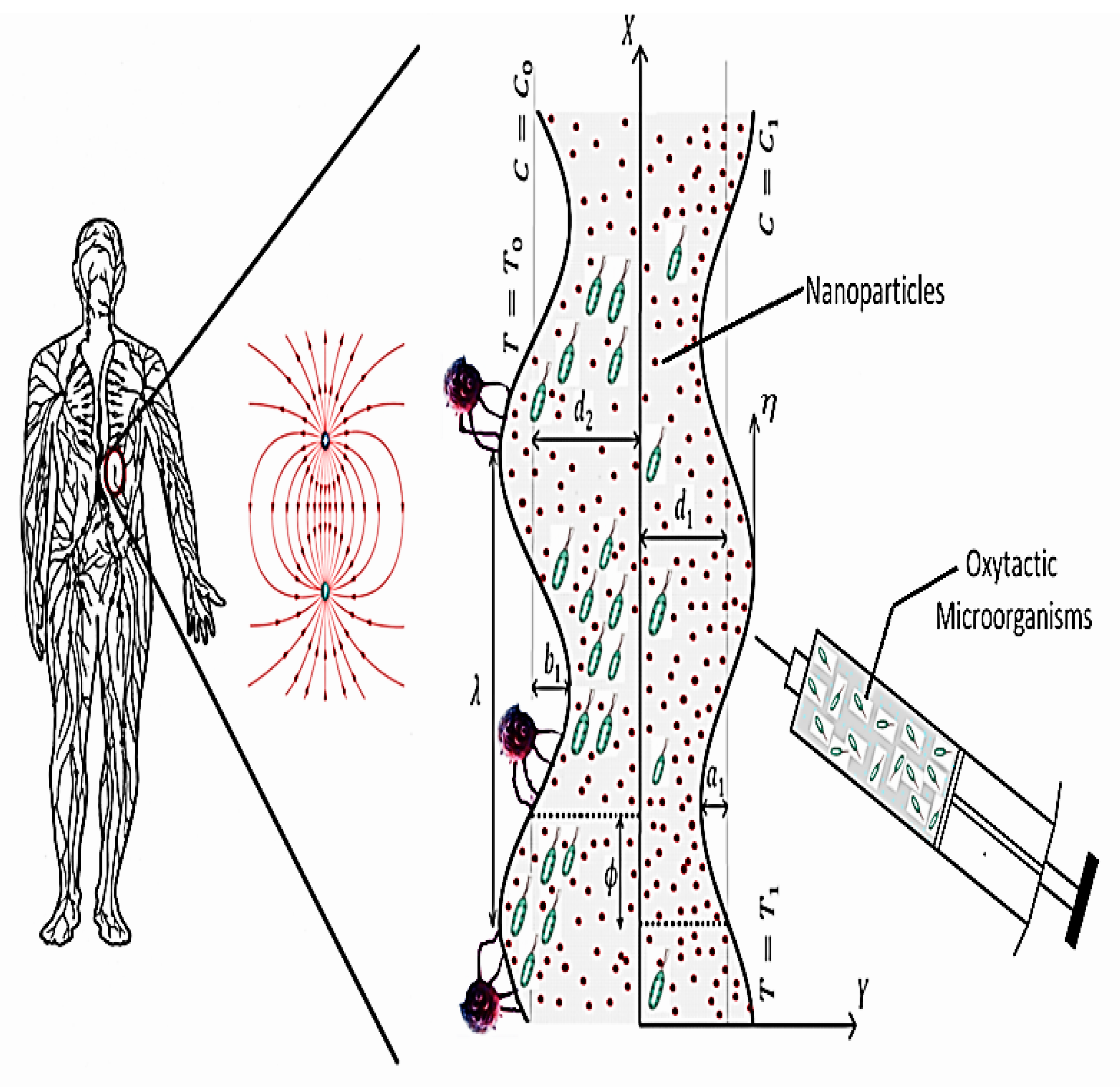
2. Physical Description

2.1. The Carreau–Yasuda Model

The constitutive equation for Carreau–Yasuda fluid [12,46,47] is given by:
S =   μ ( γ ˙ )   γ ˙   ,   μ ( γ ˙ ) = [   μ + ( μ 0   μ   ) (   1   + (   Γ   γ ˙   ) a   ) n 1 a ]   , γ ˙ = V   + ( V ) T ,   γ ˙ = | γ ˙ | = γ ˙     :   γ ˙ 2   = I   I γ ˙ 2   ,   I   I γ ˙ = t r a c e ( γ ˙ · γ ˙ ) =   i j γ ˙ i j   γ ˙ j i .
where S is the extra stress tensor, μ ( γ ˙ ) is the apparent viscosity, γ ˙ is the second invariant of the strain rate tensor, V is the velocity gradient, γ ˙ is a scalar quantity associated with γ ˙ is called the shear rate or rate of strain, μ 0 is the zero-shear rate viscosity,   μ   is the infinite shear rate viscosity, a , Γ , and n are parameters that predict the shear-thinning/thickening behavior. It is clear from the Carreau–Yasuda model that the five parameters ( μ 0 ,   μ   ,   Γ ,   n ,   a ) could be adjusted to give a perfect fit for μ ( γ ˙ ) over the whole range of γ ˙ values. As γ ˙ tends to zero, μ ( γ ˙ ) approaches the constant value μ 0 . As γ ˙ gets large, μ ( γ ˙ ) approaches the constant value μ   . Γ is a time constant parameter for the fluid that determines the shear rate at which the zero shear plateau metamorphoses to the power–law region and the transition from power–law to μ = μ   . The exponent n is a power index, n < 1 , to predict the case of shear-thinning, while for   n > 1 , the shear-thickening effect is maintained at n = 1   for ideally viscous flow behavior. The exponent a sets the size and curvature of the crossover region between the Newtonian plateau and the power–law behavior. Large values of results in an abrupt transition. For a = 2 , the model is identical to the Carreau model. In the current study, we assume that μ = 0   and thus:
μ ( γ ˙ ) =   μ 0   (   1   + (   Γ   γ ˙   ) a   ) n 1 a
Furthermore, in addition to shear rate dependence, the apparent viscosity is assumed to vary with temperature and concentration. Therefore, we consider the following expression for the viscosity [48]:
μ ( T ,   C , γ ˙ ) = μ 0   ( 1 ϵ 1 ( T T 0 ) ) ( 1 + ϵ 2 ( C C 0 ) ) (     (   1   + (   Γ   γ ˙   ) a   ) n 1 a
where T   is the temperature of the fluid, and C   is the nanoparticle concentration.   T 0   and   C 0   are reference values,   ϵ 1   and   ϵ 2   are constants related to the free activation energy of the fluid and the concentration production of nanoparticles, respectively.

2.2. Model Formulation

We consider a two-dimensional peristaltic flow of blood (Carreau–Yasuda model) in an asymmetric vertical microvessel containing oxytactic microorganisms and nanoparticles. The channel asymmetry is urged by sinusoidal wave trains of wavelength λ propagating along the channel walls with constant speed   η . A rectangle co-ordinated system ( X , Y ) is chosen such that the X -axis lies along the direction of the wave propagation, and the Y -axis transverse to it. The geometry of the flow is shown in Figure 1, and wall deformations are mathematically described as
Y = H 1 ( X , t ) =   d 1 + a 1   cos [ 2 π λ   ( X η t ) ] ,         right   wall
Y = H 2 ( X , t ) =   d 2 b 1   cos [ 2 π λ   ( X η t ) + ϕ ]   left   wall
Here a 1 and   b 1 are amplitudes of the waves.   t is the time, d 1 + d 2 is the mean width of the channel ϕ is the phase difference where 0 ϕ π . For the channel walls not to collide with each other, a 1 ,   b 1 ,   d 1 ,   d 2 and ϕ must satisfy the condition [49]:
a 1 2 + b 1 2 + 2 a 1 b 1 cos ϕ ( d 1 + d 2 ) 2
( 0 ,     n 1 , T 0 , C 0 )   and   (   1 ,     n 0 ,   T 1 , C 1   )   are the concentrations of oxygen, oxytactic microorganism density, temperature, and nanoparticle volume fractions at the left and right walls, respectively. The velocity field of the fluid   V = ( U ,   V , 0 ) . An external uniform magnetic field B = ( 0 , 0 , B 0 ) = B 0   k ^   pervaded the flow, and the Hall effects are taken into consideration. The generalized Ohm’s law can be written as [16,50]:
J = σ ( E + V × B β H   J × B )
where β H = 1 n e   e   is the Hall factor, n e is the mass of the electron, e is the charge of the electron,   σ   is the electrical conductivity of the base fluid, E is the imposed electric field,   B = B 0 + b   is the quantity   b   induces in a field produced by the current density J . In this analysis, b   is neglected in comparison with B . Moreover, assuming the total excess charges is zero, E is neglected.
Equation (7) can be solved in J to yield the Lorentz force vector in the form
J × B =   σ   B 2 0 1 + m 2   [ ( U m   V )   i ^ + ( m   U + V )   j ^   ]
m = σ   B 0   β H is the Hall parameter, i ^ ,   j ^ and k ^   are unit vectors and X , Y ,   and Z axes, respectively.
The thermal radiation effects are taken into account, and the radiative heat flux in the X   direction is considered negligible compared to the Y   direction. Hence, by using Rosseland approximation for heat radiation, the radiative heat flux q r can be written in the form:
  q r = 4     σ * 3   k *       T 4 y   j ^
where σ *   and   k * are the Stefan–Boltzmann and the Rosseland mean absorption coefficient, respectively. By assuming that the temperature differences within the flow are sufficiently small, then we can expand T 4 in a Taylor series to about   T 0 , and ignoring higher order terms we have:
T 4 4   T 0 3   T 3   T 0 4
From Equations (9) and (10) we get,
  q r = 16     σ *   T 0 3 3   k *         T y   j ^
The effects of viscous dissipations and Joule heating (Ohmic heating) are also considered in the energy equation.

2.3. Governing Equations

The equations governing the flow are described by [36,39,51,52,53,54,55]
The continuity equation
. V = 0
The momentum equation
ρ f ( V t + ( V · ) V ) = P · S + J × B + [ ( 1 C 0 ) ρ f     β T ( T T 0 ) ( ρ P ρ f ) ( C C 0 ) ( n n o )   γ 1   ( ρ m ρ f ) ]   g   ,
The heat equation
( ρ c ) f   d T d t =   . ( k T ) + S ·   V + 1 σ   J . J · q r c P     J   p · T
The nanoparticle concentration equation
d C d t = 1 ρ P   .   J   p + k 1 ( C C 0 )
The oxygen conservation equation
d d t = . [ D s ] +   ω 1 ( n n 0 )   ω 2   ( 0 )
The concentration equation for the oxytactic microorganisms
n t = . J M
where,
J p =     ρ P   D B C   ρ P   D T T m   T ,
J M =   n   V + n   ( B   W c   1 0 )   D m n .
P is the pressure, ρ f is the density of blood, ρ P is the nanoparticle density,   ρ m   is the microorganism density,   J p   is the diffusion mass flux for the nanoparticles,   J M   is the total flux of microorganisms,   C   is the nanoparticle volume fraction (also called nanoparticle concentration),   T is the temperature of blood, n   is the density of the oxytactic microorganisms,   is the oxygen concentration, γ 1   is the average volume of an oxytactic microorganism, g is the acceleration due to gravity,   β T   is the thermal expansion coefficient, D B   is the Brownian diffusion coefficient, D T   is the thermophoresis diffusion coefficient,   D m   is the diffusivity of oxytactic microorganisms,   D s   is the diffusivity of oxygen, k   is the thermal conductivity of blood, k 1   is the chemical reaction rate, B   is the chemotactic constant,   W c   is the maximum swimming speed of a microorganism (the product B W c   is assumed to be constant),   ω 1   is the oxygen production rate,   ω 2   is the oxygen break down rate, ( ρ c ) f   is the heat capacity of fluid, ( ρ c ) P is the heat capacity of nanoparticles. Although the diffusion coefficients stated above are functions in temperature and concentration, we will neglect that dependence in our study except for the oxytactic microorganisms’ diffusivity, which will be set as varying inverse to viscosity.

2.4. Transformations and Simplifications

Introducing a wave frame ( x , y ) moving with the velocity c away from the fixed frame   ( X , Y ) by the transformations,
x = X η t ,     y = Y ,     u = U η ,     v = V ,     p ( x ) = P ( X , t )
in which the boundary shape becomes stationary and ( u , v ) are the velocity components in the wave frame ( x , y ) . The stress components of the extra stress tensor S are as follows:
S x x = 2 μ 0   ( 1 ϵ 1 ( T T 0 ) ) ( 1 + ϵ 2 ( C C 0 ) ) [ 1 + Γ a   ( 2 ( u x ) 2 + 2 ( v y ) 2 + ( u y + v x ) 2 ) a 2 ] n 1 a u x
S x y =   μ 0   ( 1 ϵ 1 ( T T 0 ) ) ( 1 + ϵ 2 ( C C 0 ) ) [ 1 +   Γ a   ( 2 ( u x ) 2 + 2 ( v y ) 2 + ( u y + v x ) 2 ) a 2 ] n 1 a   (   u y +   v x   )
S y y = 2 μ 0   ( 1 ϵ 1 ( T T 0 ) ) ( 1 + ϵ 2 ( C C 0 ) )   [ 1 +   Γ a   ( 2 ( u x ) 2 + 2 ( v y ) 2 + ( u y + v x ) a 2 ) a ] n 1 a   v y
Introducing the following non-dimensional quantities:
x * = x λ   ,   y * = y d 1   ,   u * = u η   ,   v * = v δ   η ,   t * = η λ t ,       δ = d 1 λ ,   h * 1 = H 1 d 1   ,   h * 2 = H 2 d 1 , c = a 1 d 1 ,   b = b 1 d 1 ,   d = d 2 d 1 ,   p * = d 1 2 P μ 0 η λ , ψ * = ψ η d 1 ,   u * = ψ * y * , v * = δ ψ * x *   , θ = T T 0 T 1 T 0   ,   φ = C C 0 C 1 C 0 ,   Ω = n n 0 n 1 n 0 ,   ξ = 0   1 0 ,   R e 0 = ρ η d 1 μ 0 ,   μ ( θ , φ , γ ˙ ) = μ ( T ,   C , γ ˙ ) μ 0 , E c = η 2 c f   ( T 1 T 0 ) ,   ϵ 1 = β T 1 T 0   ,   ϵ 2 = α C 1 C 0 ,   σ 1 = n 0 ( n 1 n 0 )   ,     λ 1 = ω 1   ( n n 0 )   d 1 2   D s   ( Ω 1 Ω 0 ) ,   N b o = τ   D B 0   (   C 1 C 0 )   ρ f   μ 0 , N t o = τ   D T   (   T 1 T 0 )   ρ f     μ 0   T m ,   W e = Γ   η d 1   ,   R n 0 = 16     T 0 3     σ * 3   k *     μ 0     c f   ,   M 0 = σ μ 0     B 0 d 1   ,     P r 0 = μ 0     c f k , G t 0 = ( 1 C 0 ) ρ f     β   g     d 1 2 ( T 1 T 0 ) μ 0   η ,   G C 0 = ( ρ P ρ f )   g     d 1 2 ( C 1 C 0 ) μ 0   η , R b 0 = γ 1   ( n 1   n 0 ) ( ρ m ρ f )   d 1 2   g   μ 0   η , D m = D m 0   μ 1 ( θ , φ , γ ˙ )   ,     ρ e 0 = B W c D m 0   ,   λ 2 = ω 2   d 1 2   D s   ,     ϵ 0 = k 1 d 1 2   ρ f   μ 0 . .  
where μ 0   is the constant viscosity of the fluid,   ν is the kinematic viscosity of the fluid,   θ   is the dimensionless temperature, φ is rescaled nanoparticle volume fraction,   Ω   is the dimensionless density of oxytactic microorganisms,   ξ   is the dimensionless oxygen concentration,   ψ is the stream function, E c   is the Eckert number, β   is the viscosity-variation parameter with temperature,   α   is the viscosity-variation parameter with nanoparticle concentrations, W e is the Weissenberg number, σ 1   is the bioconvection constant, R e 0 ,   P r 0 ,   M 0 , N b 0 , N t 0 , G t 0 , G C 0 , R b 0 ,   R n 0 ,   ρ e 0   ,   ϵ 0 are Reynold’s number, the Prandtl number, the Hartman number, the Brownian motion parameter, the thermophoresis parameter, the temperature Grashof number, the mass Grashof number, bioconvection Rayleigh number, the thermal radiation parameter, the bioconvection Peclet number, and the chemical reaction parameter at constant viscosity   μ ( T ,   C , γ ˙ ) = μ 0 .
By invoking the assumptions that the wavelength is large ( δ   1 ) , and the Reynold’s number is low ( R e 0 < 1 )   we then use Equations (3), (8), (11), (18), (19) and (24) in Equations (12)–(17) and drop the asterisks. The continuity equation is identically satisfied, and the resulting system of equations in simplified form can be written as follows:
p x = y [ ( 1 β θ ) ( 1 + α   φ ) [   1 + ( n 1 )   W e a a   ( 2 ψ y 2 ) a   ]     2 ψ y 2   ] M 0 2 1   +   m 2   ( ψ y + 1 ) + G t 0   θ G c 0   φ     R b 0   Ω ,
0 =   p y
0 = ( 1 P r 0 + R n 0 ) 2 θ y   2 + E c   ( 1 β θ ) ( 1 + α   φ ) [   1 + ( n 1 )   W e a a   ( 2 ψ y 2 ) a   ]   ( 2 ψ y 2 ) 2 + E c   M 0 2 1   +   m 2   ( ψ y + 1 ) 2 + N b 0 θ y φ y + N t 0   ( θ y ) 2 ,
0 = N t 0   2 θ y   2 + N b 0 2 φ y   2 ϵ 0   φ ,
0 = 2 ξ y   2 + λ 1 Ω   λ 2 ξ ,
0 = y [ ( 1 α   φ ) ( 1 + β θ ) [   1 ( n 1 )   W e a a   ( 2 ψ y 2 ) a   ]     Ω y   ] ρ e 0 ( Ω y   ξ y +   Ω   2 ξ y 2 + σ 1   2 ξ y 2   ) ,
From Equation (23) ,   p   is not a function of y , and hence, one can eliminate pressure in Equation (22) and obtain
0 = 2 y   2 [ ( 1 β θ ) ( 1 + α   φ ) [   1 + ( n 1 )   W e a a   ( 2 ψ y 2 ) a   ]     2 ψ y 2   ] + y [   M 2 1   +   m 2   ( ψ y + 1 ) + G t 0   θ G c 0   φ R b 0   Ω   ] .

2.5. Variable Non-Dimensional Parameters

By checking out the definitions of the Prandtl number, Hartman number, Grashof number, local mass Grashof number, Brownian motion parameter, thermophoresis parameter, bioconvection Peclet number, Thermal radiation parameter, chemical reaction parameter, and bioconvection Rayleigh number for oxytactic microorganisms, we recognize that these non-dimensional parameters are functions of viscosity. Since viscosity is assumed to vary across the flow, then these mentioned parameters will vary, too. Ignoring such phenomena will lead to unrealistic results [28].
Accordingly, the parameters mentioned above relate to the variable viscosity and can be written as follows:
P r v =   c f   μ     K =   c f   μ 0 K   Λ = P r 0   Λ
M v = σ μ     B 0   d 1 = ( σ μ 0   Λ       ) 1 / 2 B 0   d 1 =   M 0   ( 1   Λ     ) 1 / 2 ,
R b v = γ 1   ( n 1   n 0 ) ( ρ m ρ f )   d 1 2   g   μ   η = γ 1   ( n 1   n 0 ) ( ρ m ρ f )   d 1 2   g   μ 0   η   Λ = R b 0     Λ ,
R n v = 16     T 0 3     σ * 3   k *     μ     c f       =   16     T 0 3     σ * 3   k *     μ 0     c f     Λ     = R n 0 Λ ,
G t v = ρ f     β   g     d 1 2 ( T 1 T 0 ) ( 1 C 0 ) μ   η = ρ f     β   g     d 1 2 ( T 1 T 0 ) ( 1 C 0 ) μ 0   η   Λ =   G t 0   Λ ,
G c v = ( ρ P ρ f )   g     d 1 2 ( C 1 C 0 ) μ   η = ( ρ P ρ f )   g     d 1 2 ( C 1 C 0 )   η   μ 0     Λ = G c 0       Λ ,
N b v = τ   D B   (   C 1 C 0 )   ρ f   μ = τ   D B   (   C 1 C 0 )   ρ f   μ 0   Λ =   N b o Λ   ,
N t v = τ   D T   (   T 1 T 0 )   ρ f μ     T m =   τ   D T     (   T 1 T 0 )   ρ f μ 0   Λ   T m =   N t o Λ ,
ϵ v = k 1 d 1 2   ρ f   μ = k 1 d 1 2   ρ f   μ 0   Λ = ϵ 0     Λ   ,
D m =   D m 0 Λ   ,
ρ e v = B   W c D m =   B   W c     D m 0     Λ   = ρ e 0 Λ   ,
where
Λ = ( 1 β θ ) ( 1 + α   φ ) [   1 + ( n 1 )   W e a a   ( 2 ψ y 2 ) a   ]
Substituting Equations (32)–(43) with Equations (25), (27)–(31), we obtain the following modified system of equations:
d P d x = y [   Λ     2 ψ y 2   ] + ( G t v   θ M v 2 1   +   m 2   ( ψ y + 1 ) G c v   φ R b v   Ω )   Λ ,
0 = ( 1 P r v + R n ) 2 θ y   2 + E c     ( 2 ψ y 2 ) 2 + E c   M 2 1   +   m 2   ( ψ y + 1 ) 2 + N b v   φ y θ y + N t v   ( θ y ) 2
0 = N t v   2 θ y   2 + N b v   2 φ y   2 ϵ v   φ ,
0 = 2 ξ y   2 + λ 1 Ω   λ 2 ξ ,
0 = y [   Λ   Ω y   ] ρ e v   Λ · ( Ω y   ξ y +   Ω 2 ξ y 2 + σ 1   2 ξ y 2   ) ,
Equation (44), after eliminating pressure, becomes the following:
0 = 2 y   2 [ Λ     2 ψ y 2   ] + y [ ( G t v   θ M v 2 1   +   m 2   ( ψ y + 1 ) G C v   φ R b v   Ω ) Λ ]
We denote the system of Equations (44)–(49) by the “variable parameters model” (VP-Model). In comparison, we labeled the system of Equations (25)–(31) as the “constant parameters model” (CP Model) in which the parameters that function in viscosity are treated as constants.
Notice that both systems, the CP—Model and the VP-Model, are reduced to a typical set of equations that corresponds to the case of a Newtonian fluid with a constant viscosity by setting β , α ,   and W e equal to zero.

2.6. Boundary Conditions

The appropriate boundary conditions for both the CP—Model and the VP-Model in the dimensionless form are as follows:
ψ y = 1 ,     ψ = q 2 ,     θ = 1 ,     φ = 1 ,     ξ = 1 ,     Ω = 0 ,   at   y = h 1 = 1 + c   cos ( 2   π x ) ,
ψ y = 1 ,     ψ = q 2 ,     θ = 0 ,   φ = 0 ,     ξ = 0 ,     Ω = 1 ,   at   y = h 2 = d b cos ( 2   π x + ϕ ) ,
where a , b , d and ϕ satisfy the relation,
a 2 + b 2 + 2 a b   cos   ϕ ( 1 + d ) 2
The dimensionless mean flow over one period in the fixed frame Q   and in the wave frame   q   are related by [56]:
Q   = 1 + d + q ,
in which
q =   h 2 h 1 u d y

3. Results and Discussion

The system of Equations (25)–(31) labeled as the CP-Model and the system of Equations (44)–(49) labeled as the VP-Model, along with the boundary conditions Equations (50) and (51), were solved numerically with the aid of the most sophisticated version of the computational software program Mathematica 11.3. The obtained solutions via the built-in command ParametricNDSolve were displayed through Figure 2, Figure 3, Figure 4, Figure 5, Figure 6, Figure 7, Figure 8 and Figure 9 to analyze the problem’s physics. Parametric study for both the CP-Model and the VP-Model on temperature, nanoparticles volume fraction, microorganism density profiles, longitudinal velocity, and longitudinal pressure gradients is carried out. The selected values for all embedded parameters are in Figure 2, Figure 3, Figure 4, Figure 5, Figure 6, Figure 7, Figure 8 and Figure 9 (see Table 1 and Table 2).
In the following subsections, we are going to perform the following:
(1)
Show that the VP-Model is more reliable than the CP-Model.
(2)
Investigate the features of adding oxytactic microorganisms (as oxygen repellents) to the upstream of the blood flow.
(3)
Examine the magnetic field parameters’ role in the presence/absence of the Joule heating effect for the VP-Model case.
(4)
Discuss the theoretical significance of the current study’s ambient parameters supported with experimental agreements and theoretical studies whenever possible.

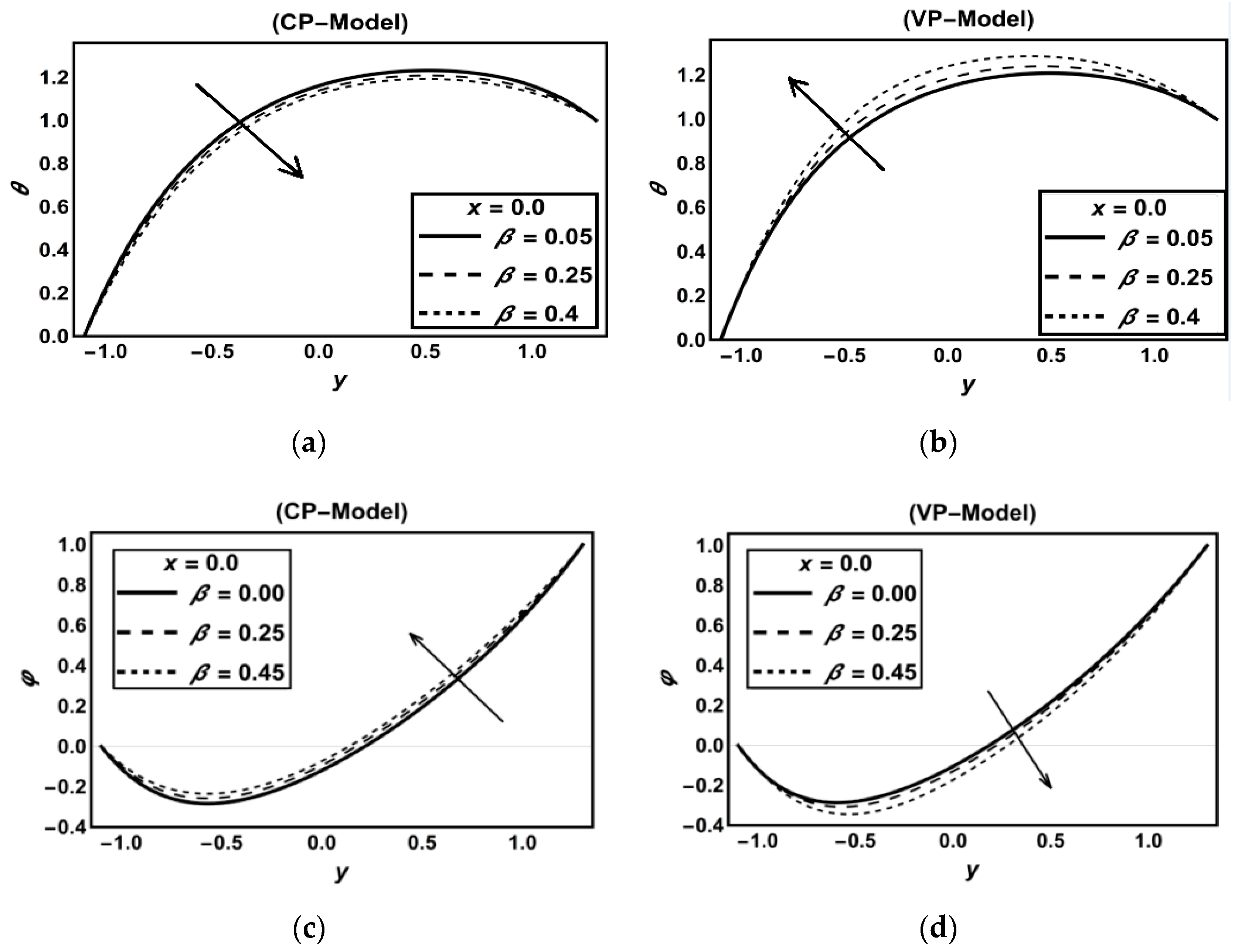
3.1. CP-Model Versus VP-Model

We made several comparisons to check the reliability of the VP-Model over the CP-Model. These comparisons were made by setting adjustable values for the parameters previously defined for the CP-Model and then assigning the same values for their corresponding ones in the VP-Model. Then, one favorable chosen parameter can take the same values in both models to realize its effect on the physical quantity under consideration. Then we have two possible scenarios in each comparison. In the first scenario, the displayed figures show the same behaviors with different magnitudes for both CP-Model and the VP-Model. In the second scenario, opposite behaviors were observed between both models. Indeed, we are interested in the second scenario, which settles the issue. For this purpose, we prepared Figure 2a–d.
Figure 2a–d display the effect of the temperature-viscosity variation parameter β   on the temperature θ , and the nanoparticle concentration φ for both the CP-Model and the VP-Model. Figure 2a elucidates that for the CP-Model, by increasing β (i.e., the viscosity decreases), the temperature θ decreases. While the converse is noticed in the VP-Model case, as shown in Figure 2b, here, the observation concerning the VP-Model is physically satisfied, as the liquids’ viscosity decreases by increasing the temperature. This is because the liquid molecules gain more energy at higher temperatures and move more freely [57,58]. It is noticeable from Figure 2c,d that the nanoparticle concentration increases by increasing β in the CP-Model case while it decreases by increasing β in the VP-Model case. Again, we found out that the case of the VP-Model follows the real situation. The increase in intermolecular distances due to thermal expansion accompanied by temperature increase results in decreasing concentration. Therefore, from the above discussions, we conclude that the CP-Model case leads to unrealistic results, whereas the VP-Model shows real outcomes.

Discussion on Some Previous Works

Elogail and Elshekipy [28] caught sight of the necessity of treating the non-dimensional parameters that rely on viscosity in their definitions in the set of governing equations to be variables too. Consequently, this extra step has modified the set of governing equations (as in the VP-Model). Fortunately, this reasonable modification has led to real results. Some published papers in the peristaltic literature have recently involved the effects of the temperature-dependent viscosity in their analysis. The way these researchers had constructed their analysis is similar to our procedure, getting the CP-Model in the present study. Herein, we refer to unrealistic outcomes that appear in their attempts as in Hayat et al. ([23], Figure 3a, page 1588)), Hussain et al. ([24], (Figure 5a, page 14), (Figure 6a, page 15)), Alvi et al. ([25], (Figure 6a, page 1119), (Figure 8a, page 1121)), Abbasi et al. ([26], Figure 10a, page 2180) and Hayat et al. ([27], Figure 13, page 222). In all the figures mentioned above, it is clear that a temperature decrease accompanies a decrease in fluid viscosity (see Refs. [23,24,25,26,27]), whereas an increase in viscosity corresponds to lower concentration values (see Refs. [24,25]). These results are unrealistic, as we noticed in Section 3.1. On the other hand, we considered the novelty of such an idea in the present work (VP-Model). We will perform further comparisons in the up-coming sub-sections to show that our obtained results in the VP-Model case follow the physical agreements, unlike those obtained in the CP-Model case.

3.2. Oxytactic Microorganism Parameters

This section has shown the physical significance of the parameters associated with the oxytactic microorganism phenomenon through Figure 3a–h. Figure 3a depicts that the density of oxytactic microorganisms is an increasing function of the Peclet number ρ e v . As the viscous forces dominate the blood flow in microvessels, and since the microorganisms diffusion is in inverse proportion to viscosity. Hence, an increment in ρ e v corresponds to a decrease in the diffusivity of the microorganisms, and consequently, microorganism density increases. Figure 3b illustrates that the microorganism density profile Ω gets increased when the biconvection constant σ 1   is increased (i.e., by increasing the ratio n 0 to n 1 ). Figure 3c declares that an increase in the production rate of oxygen leads to a boost in the microorganism density profile. By plotting the rate of change of Ω   ( i . e . ,   d Ω / d y )   versus y for several values of λ 1   as in Figure 3d, we have captured more details about Figure 3c. That is, in Figure 3d, as long as λ 1   is increased, the density of microorganisms decreases more rapidly near high oxygen concentrations (at the right microvessel wall). While near low oxygen concentrations (at the left microvessel wall), microorganism density increases most rapidly. Figure 3e,f display the variation of Ω   and d Ω / d y   versus y for several values of the breakdown rate λ 2 ( λ 2   represents a reference value for the concentration of oxygenation below which the microorganisms will not respond to the oxygen gradients stimulus). These figures show that the effect of λ 2 on Ω   and d Ω / d y is quite the opposite behavior to that of   λ 1 . Figure 3g,h give an insight into the variations of temperature and longitudinal velocity for different values of the bioconvection Raylight number R b v . It is evident that the temperature increases with a rise in R b v .   It is also clear that the extreme values of the velocity are shifted towards the right microvessel wall by assigning higher values to R b v .

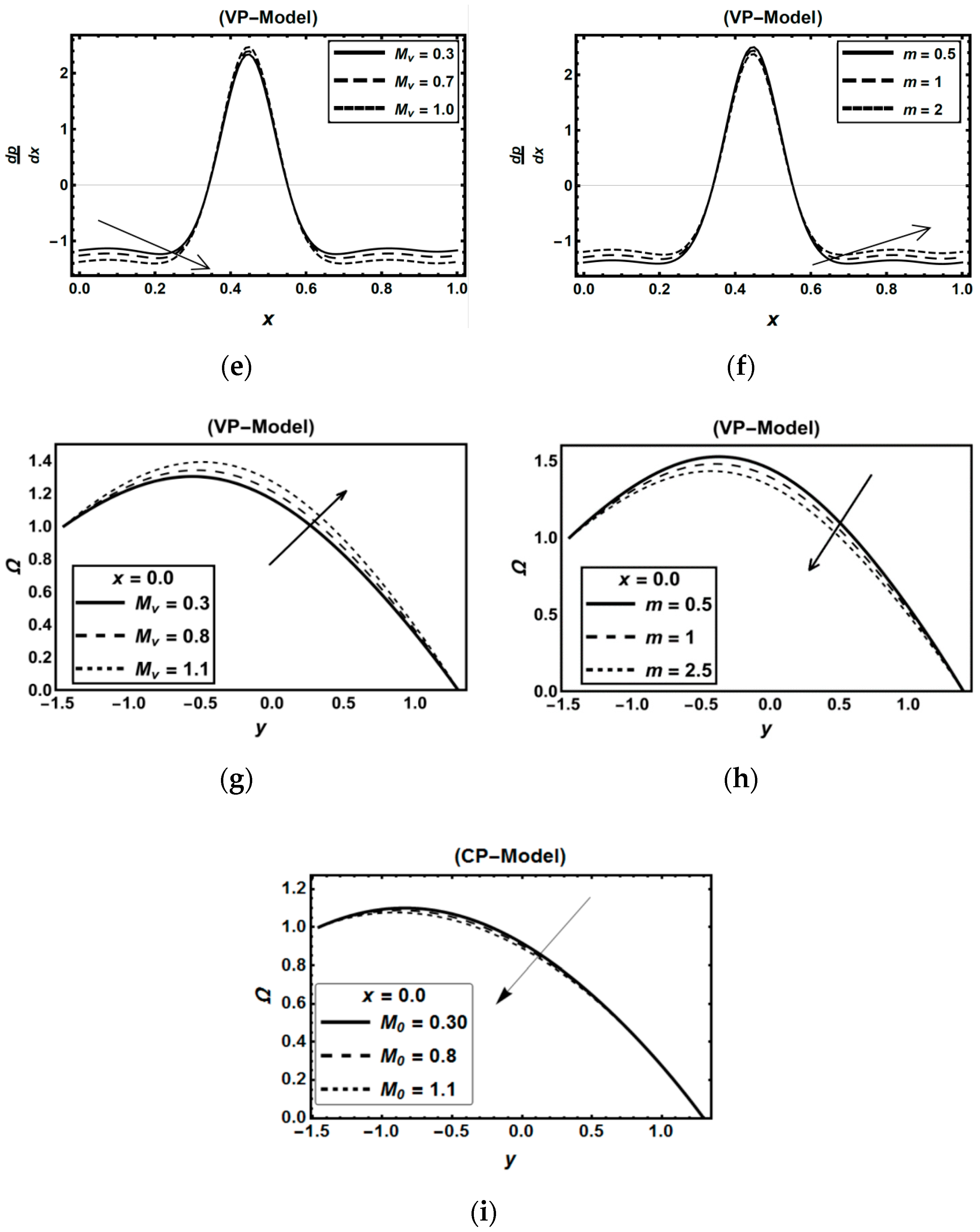
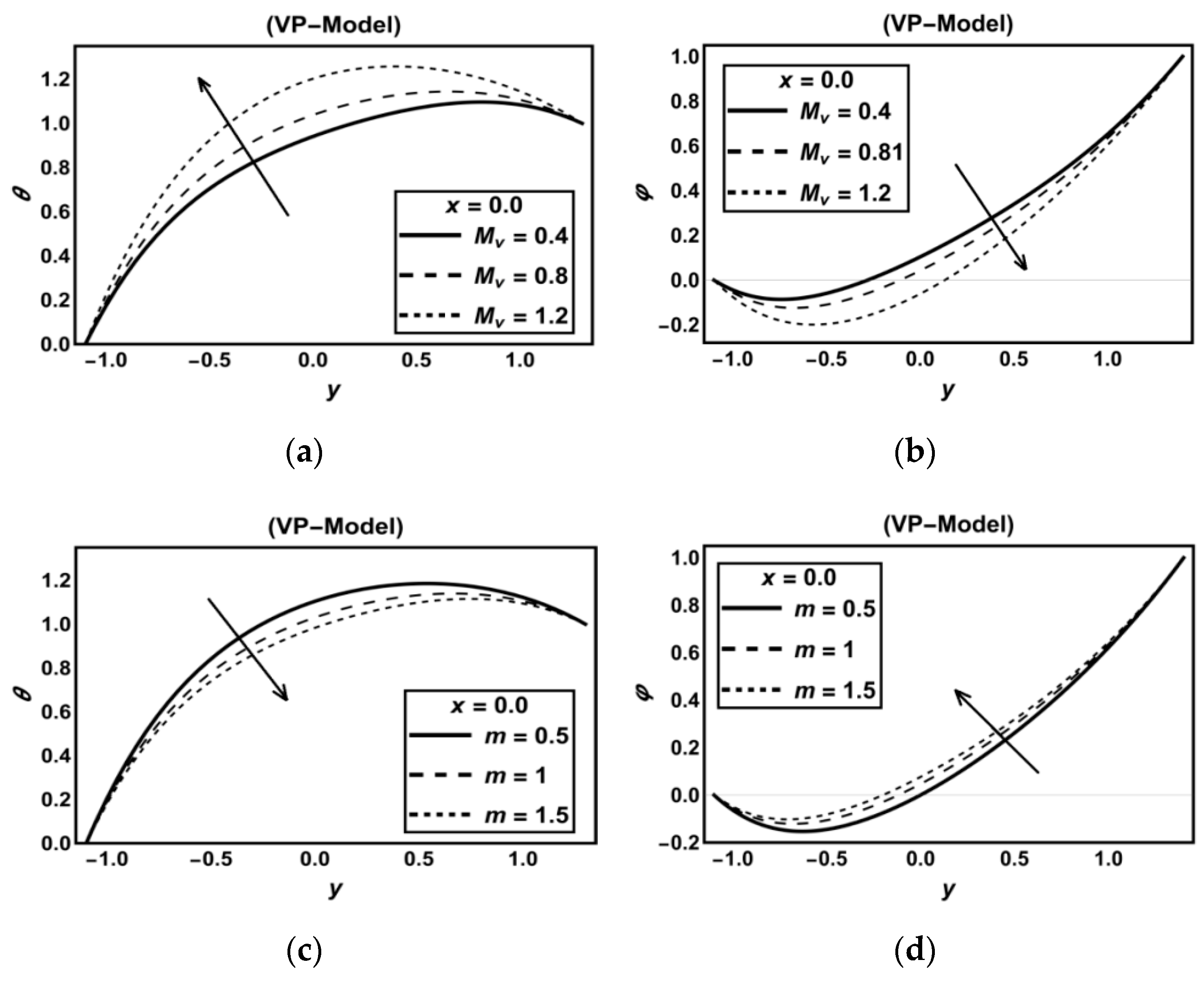
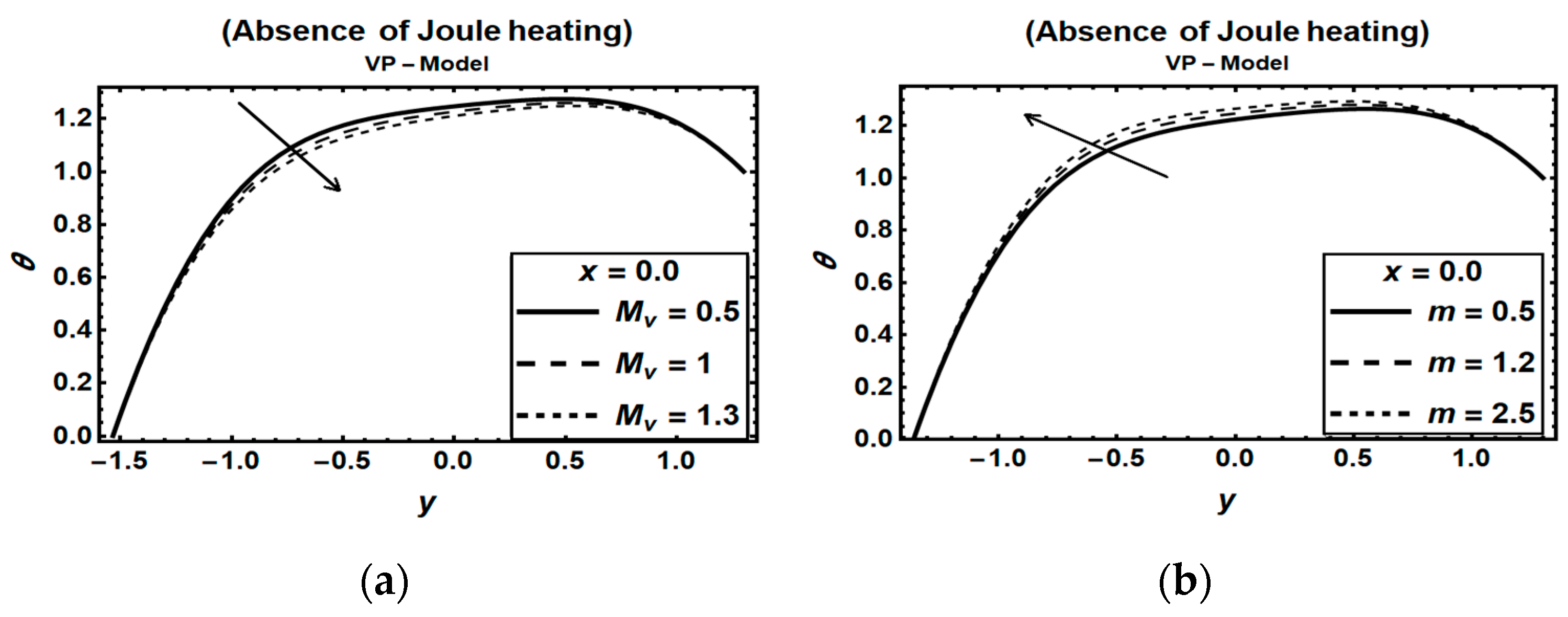
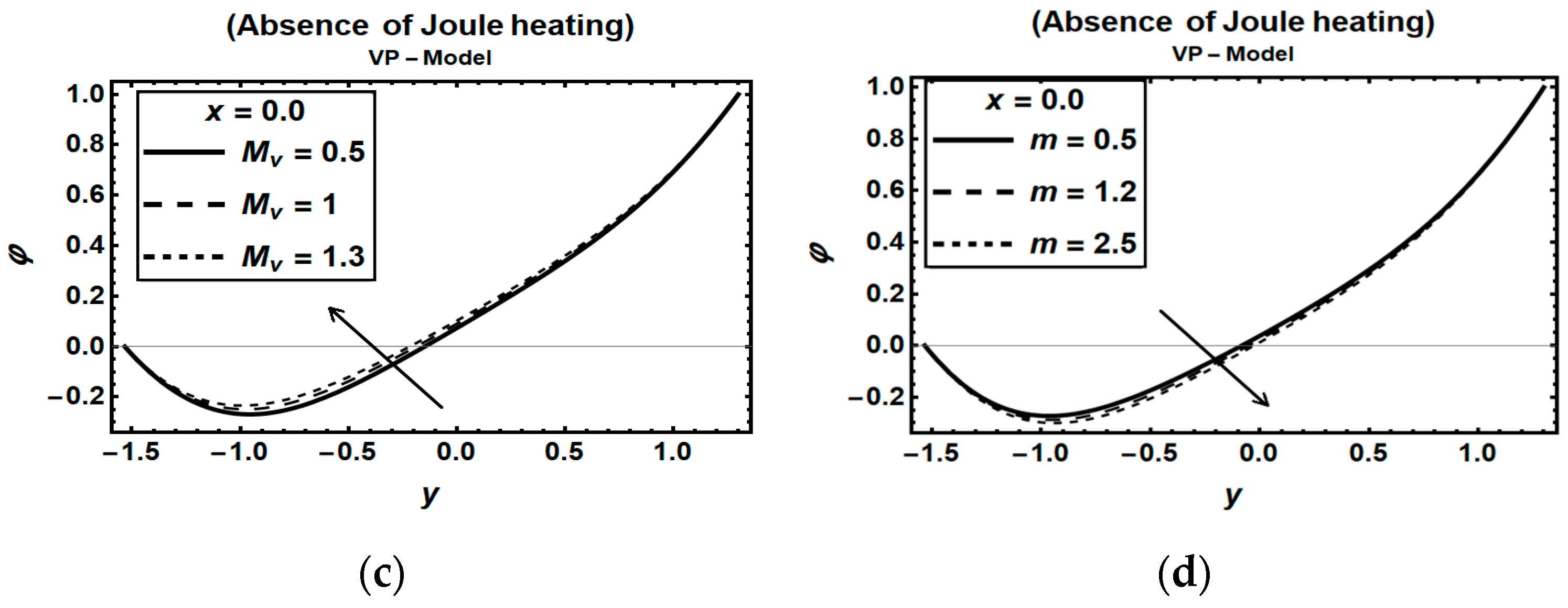
3.3. Magnetic Field Parameters and Joule Heating Effects

During Joule heating, electric currents pass through the electrically conducting fluid, and the resistance it enforces results in heat generation within the flow. It is worth mentioning that ignoring the effects of such a phenomenon during the study of electrically conducting liquids stressed by magnetic fields may lead to significant errors in the obtained results.
In the current investigation, we were eager to examine the above notice for the VP-Model case. Hence we analyzed the impacts of the Hartman number M v and the Hall parameter m in the presence/absence of the Joule heating effect in the energy equation in two different cases. In the first case, we prepared Figure 4a–i (First Case (Presence of Joule Heating)) to see the variation in the temperature and nanoparticle concentration for several Hall parameter values and the Hartmann number considering the Joule heating effect. Figure 4a,b llustrate that by increasing the Hartmann number, the temperature increases, while the nanoparticle concentration decreases. The results displayed in Figure 4c,d indicate that when the Hall parameter values increase, the nanoparticle concentration increases, whereas a decrease in the temperature is noticed. In the second case, we have omitted the Joule effect term from the heat equation, then recalculated the effects of the Hartmann number and the Hall parameter on the temperature and concentration profiles. In this case, the results, as displayed in Figure 5a–d (Second Case (Absence of Joule Heating)), have shown the opposite trend in considering the Joule heating effect.
Figure 4e–h were made to analyze the effects of the Hartman number M v   and the Hall parameter m on the longitudinal pressure gradient   d p / d x   and the microorganism density profile   Ω . Figure 4e,f exhibit that when M v   increases, the pressure gradient decreases in the broader part of the channel, whereas a slight increase in the pressure gradient is realized in its narrow part. The influence of increasing the Hall parameter on the pressure gradient d p / d x shows quite the opposite behavior to that of Hartmann number   M v . From Figure 4g,h it can be seen that larger values of the Hartmann number M v   magnify the microorganism density. This is due to the dominance of the Lorentz forces in reducing the blood flow. The Hall parameter’s increasing values show decreased microorganism density (see Figure 4h). Physically, this is for the reason that an increase in m will result in reducing the electrical blood conductivity through the term ( σ / ( 1   +   m 2 ) ) .   This generates a magnetic damping force, which enhances the blood velocity. The comparison of Figure 4g with Figure 4i shows another unrealistic observation for the case of the CP-Model.

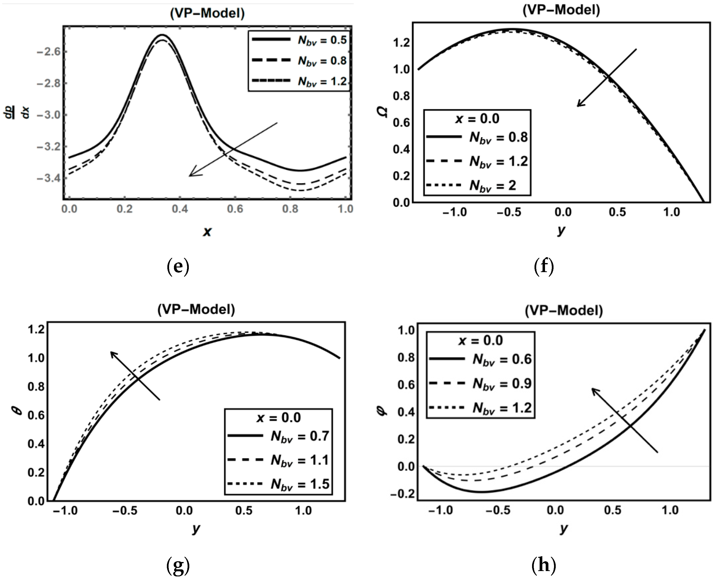
3.4. Role of Nanoparticles Parameters

We have plotted Figure 6a–h to visualize the effects of the Brownian motion parameter N b v and the thermophoresis parameter N t v   on the longitudinal pressure gradient   d p / d x , temperature θ, nanoparticle concentration   φ , and microorganism density   Ω . Figure 6a–c display that the larger values of N t v   show an enhancement in d p / d x   , θ ,   and   Ω . It is clear from Figure 6d that the nanoparticle concentration decreases with an increase in N t v . The magnitude of d p / d x   and Ω   decreased by increasing   N b v ,   as shown in Figure 6e,h. It is clear from Figure 6g,h that θ and φ boost by an increase in   N b v . Generally, a continuous increase in random collisions between the molecules and particles of bulk fluid enhances the fluid’s thermal conductivity. That is why the temperature and nanoparticle concentration profiles increase when increasing the Brownian motion parameter.

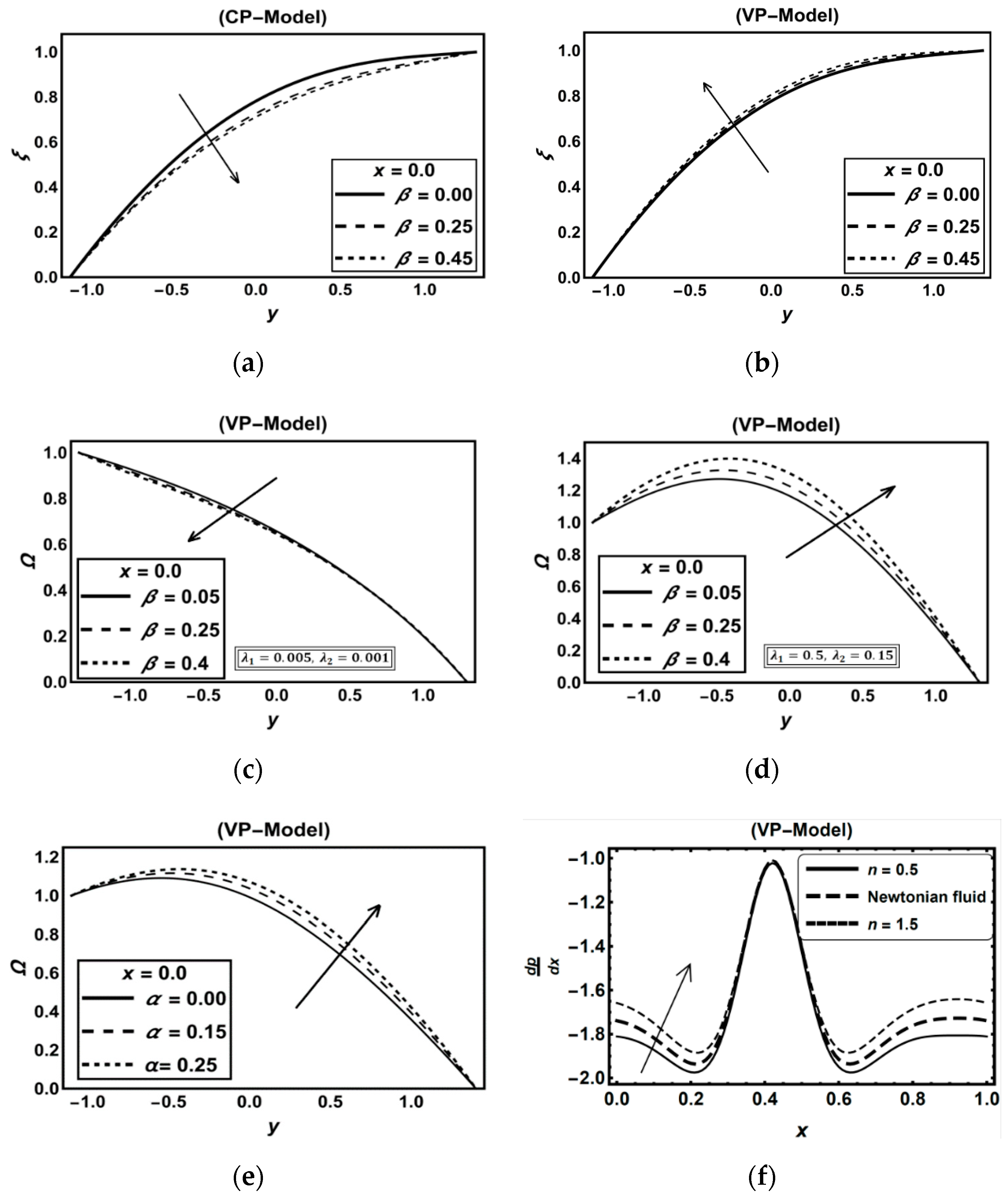
3.5. Role of Carreau–Yasuda Fluid Parameters

In this section, we intend to elaborate on the Carreau−Yasuda fluid parameters’ roles, namely the viscosity-variation parameter with temperature   β ,   the viscosity-variation parameter with nanoparticles volume fraction α , the Weissenberg number W e ,   the power low index n   and the Carreau—Yasuda exponent a . For this purpose, Figure 7a–j were prepared. In Figure 7a,b, a comparison between the VP-Model and the CP-Model was performed to investigate the oxygen concentration profile ξ for various values of   β . Figure 7a indicates that an increase in β   results in a decrease in ξ for the case of the CP-Model. Whereas, an increase in β   marks an increasing behavior in ξ for the VP-Model, as illustrated in Figure 7b. The last observation for the VP-Model was investigated by Marini et al. [59] They concluded that an increase in blood viscosity could alter and compromise cellular oxygen transfer. In another attempt, Most et al. [60] reached experimentally the conclusion that a reduction in blood viscosity could exert a favorable influence on maximal oxygen delivery. Inspired by this information, a reduction in blood viscosity will improve the oxygen-carrying capacity in hypoxic regions. Consequently, the oxygen-repellent microorganisms that could encapsulate drugs will be directed to spread over the tumor tissues’ targeted cells. Indeed, the comparisons made between the CP-Model and the VP-Model in Section 3.1 and in this Section 3.5 strengthen our assumptions on the variable-parameters case discussed formerly in Section 2.5. In Figure 7c, it is quite noticeable that the microorganism density profile   Ω decreases when increasing β (i.e., Ω   decreases by a decrease in the blood viscosity). However, and under the same circumstances considered in Figure 7c, when boosting the oxygen concentrations within the streamflow, Ω is increased and directed to hypoxic regions (see Figure 7d). That tells us that, regardless of the increase in β values, sufficient gains in the oxygen concentrations in the tumor vasculature will dominate the decrease in the blood viscosity and directed the oxygen-repellent microorganisms towards the hypoxic tumor cells. In Figure 7e, the effect of the viscosity-variation parameter with nanoparticle volume fraction on   Ω is displayed. We notice from this figure that increasing α   results in an increase in Ω . The effects of the Weissenberg number W e ,   the power low index n   and the Carreau–Yasuda exponent a on the axial velocity u are computed in Figure 7f–j. It is clear from Figure 7f that the case of blood shear thickening ( n > 1 ) has a higher value of pressure gradient at the broader part of the blood-vessel x [ 0 ,   1 ]   [ 0.55 ,   1 ] when compared with the shear thinning case ( n < 1 ) , while there are no noticeable differences at the narrow part of the blood-vessel   x [ 0.35 ,   0.5 ] . Figure 7g,h were prepared to depict the influence of W e   on axial velocity u   for both shear thinning and shear thickening. Figure 7g shows that an increase in W e   for shear thinning blood results in a decrease in the axial velocity at the right half of the channel, whereas it increases at the left part of the channel. On the other hand, the longitudinal velocity has the opposite behavior for shear thickening blood, as illustrated in Figure 7h. Interestingly, Figure 7i presents the variation of pressure gradient over one wavelength for various values of   a . It is clear that with an increase in the value of a   from a = 1 to a = 2 ,   the pressure gradient increases significantly at the broader part of the blood vessel, while little change was observed at the narrow part of the blood vessel. Upon a further increase in a upon substituting positive constitutive integer values ( a = 3 ,   a = 4 ), the pressure gradient starts showing an alternating increase/decrease behavior in the blood vessel broader part. In contrast, no noticeable change is regarded in the narrower part. The maximum pressure gradient occurs in the case of the Carreau fluid   ( a = 2 ). We have also plotted the effect of varying   a   on the longitudinal velocity u ,   as shown in Figure 7j. This figure reflects that the velocity   u goes faster near the right microvessel wall in response to increasing values of a   whereas a decline in u near the left microvessel is evident.

3.6. Role of Thermal Radiation, Buoyancy, Chemical Reaction and Flow Rate Effects

This section exhibits graphical depictions that feature effects of the thermal radiation parameter   R n v , the mass Grashof number   G c v , the temperature Grashof number   G t v ,   the chemical reaction parameter, and the dimensionless flow rate parameter   q . The role of the thermal radiation parameter   R n v   on nanoparticle concentration and temperature profiles are demonstrated in Figure 8a,b. Clearly, for a higher estimation of   R n v values, the nanoparticle concentration increases while the temperature lessens. This is because an increase in the   R n v parameter corresponds to a decrease in the mean absorption coefficient   k * and hence, temperature decreases. Figure 8c,d are plotted to realize the characteristics of generative ( ϵ v < 0 ) / destructive ( ϵ v > 0 ) chemical reaction parameter ϵ v on temperature θ and nanoparticle concentration φ   distributions. Figure 8c shows a decrease in φ   because of a destructive (bond breaking) chemical reaction. However, an enhancement in φ   is seen in the case of a generative chemical reaction (bond making). Figure 8d portrayed that the temperature distribution rises for a generative chemical reaction and retards for a destructive chemical reaction. As a matter of fact, bond breaking is an endothermic reaction (i.e., it requires energy for the reaction to occur fully). Hence, the reaction proceeds with the net absorption of heat from the surrounding medium, and thus temperature decreases. On the other hand, by applying the law of mass—energy conservation, losing energy from the system to the surroundings (as in exothermic reaction) will be compensated by gaining extra mass by the reacting system. For the case of bond destructing (endothermic reaction), energy is absorbed by the system from the surrounding medium, and consequently, a decrease in the concentration is noticed. Figure 8e announces that there is an increase in the longitudinal pressure gradient   d p / d x when G t v is increased. The effect of G c v   on d p / d x is opposite to the impact of G t v   (see Figure 8f). Figure 8g shows that the microorganism density profile increases in a generative reaction rather than a destructive reaction. Figure 8h characterizes the influence of the rate of flow parameter q on the longitudinal pressure gradient   d p / d x . This figure elucidates that for higher q   rates it is noticed that d p / d x   decreases. This last observation is consistent with the outcomes of Asha and Sunitha [61].

3.7. Streamlines and Trapping

The trapping phenomenon is an interesting topic to any peristaltic flow in which closed streamlines formulate an internally circulating bolus. This trapped bolus moves forward along with the peristaltic wave. This mechanism has a great significance in physiology, as this mechanism is favorable for the formation of thrombus in the blood, pathological movement of bacteria, etc. This phenomenon is analyzed in Figure 9a–c. It is recorded from Figure 9a that, as the viscosity variation parameter with temperature β increases, the streamline circulations get stronger. Subsequently, the size and number of trapping bolus rise, revealing that the viscosity-dependent on temperature plays an essential role compared with the constant viscosity. The effect of the viscosity variation parameter with nanoparticle concentration α on trapping can be seen in Figure 9b. From this figure, it is observed that, by raising the values of α , a vice versa of the β effect occurs, i.e., the number of trapping bolus decreases, and their sizes become smaller. Figure 9c represents that when the Hartmann number M v increases, the circulation and size of the trapping bolus gradually decreases, and that the fluid moves as a bulk for higher values of M v . Thus, formations of circulating bolus can be controlled using an adjustable magnetic field force.

4. Conclusions

We have developed a novel mathematical model simulating microvascular blood flow with oxygen-repellent microorganisms and nanoparticles in the presence of a magnetic environment. The blood viscosity is considered to vary with temperature, nanoparticle concentration, and shear strain. The microorganisms’ diffusivity is assumed to change inverse to viscosity. Effects of Hall current, Joule heating, thermophoresis, Brownian motion, thermal radiation, viscous dissipations, and 1st order chemical reactions were taken into account. The coupled non-linear differential equations governing the problem were set in a dimensional form, simplified under long-wavelength assumptions and low Reynold’s numbers. Then these equations are labeled as the CP-Model. However, it seems more realistic to consider all non-dimensional parameters in the CP-Model defined in terms of viscosity to be variables. Accordingly, we obtained a new system of equations that we labeled as a VP-Model. Solutions for the VP-Model have been obtained and are displayed through plots via the software program Mathematica 11.3 by implementing the built-in command “ParametricNDSolve”. Comparisons between the CP-Model and the VP-model were carried out. Lastly, we discussed the effects of various parameters, and the significant findings are summarized as follows:
(1)
We have confirmed the VP-Model’s reliability over the CP-Model by referring to physical phenomena and past experimental results.
(2)
Disregarding the Joule heating effects in modeling MHD flow problems in the presence of heat and mass transfer will result in unrealistic outcomes.
(3)
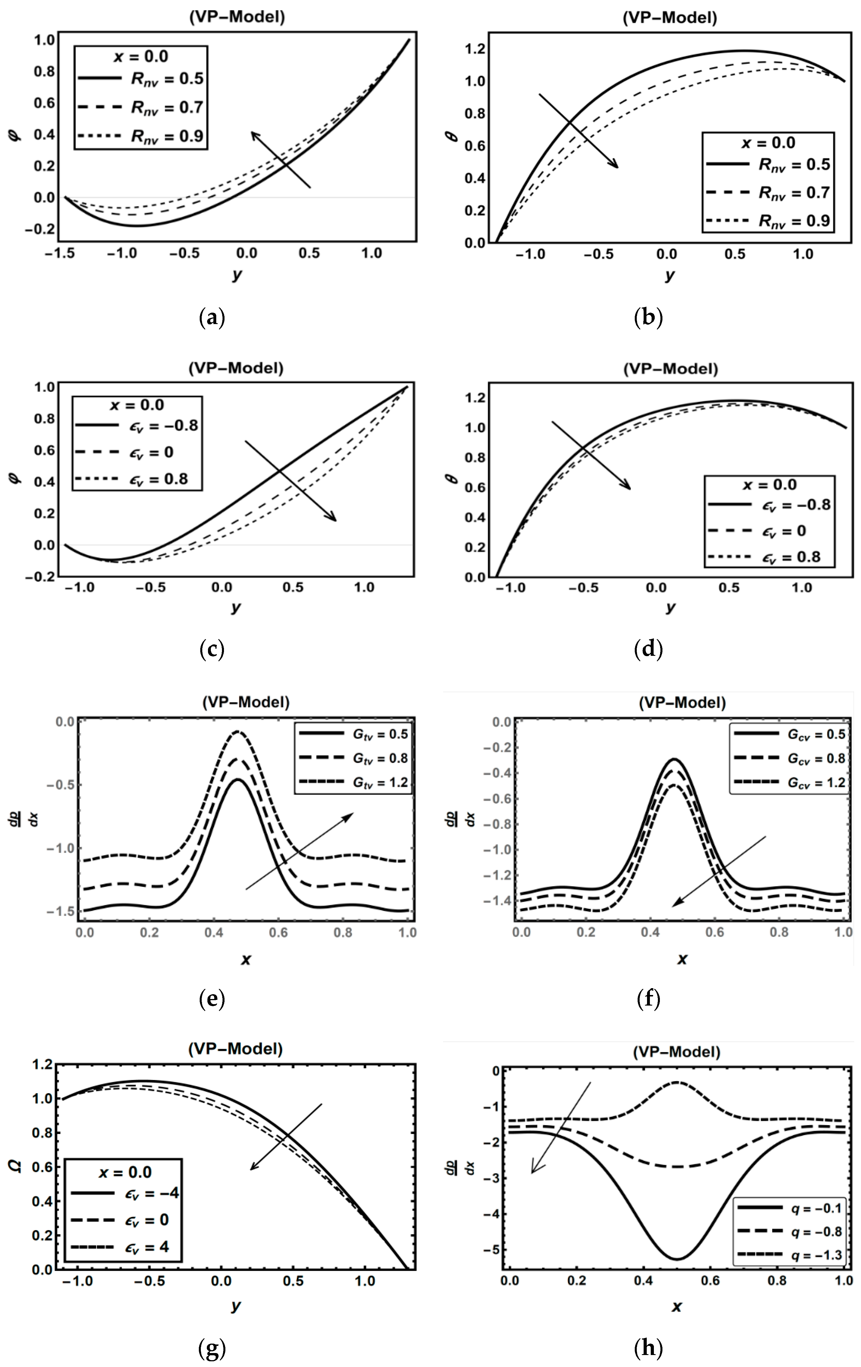
Microorganism density is an increasing function of   N t v   ,     α ,   σ 1 , ρ e v ,   λ 1   and   M v , whereas it decreases with increasing   λ 2 ,     N b v and   m .
(4)
Rising in oxygen concentrations causes the microorganism density to increase in the direction towards the hypoxic tumor regions; even a reduction in blood viscosity is regarded.
(5)
The impacts of   N t v   on the temperature and nanoparticle volume fraction profiles are quite the opposite. On the other hand, the influences of N b v   on the nanoparticle volume fraction and temperature profiles are similar.
(6)
In the presence of a generative chemical reaction, the temperature, nanoparticle concentration, and microorganism density profiles are boosted, but the opposite trend occurred for a destructive chemical reaction.
(7)
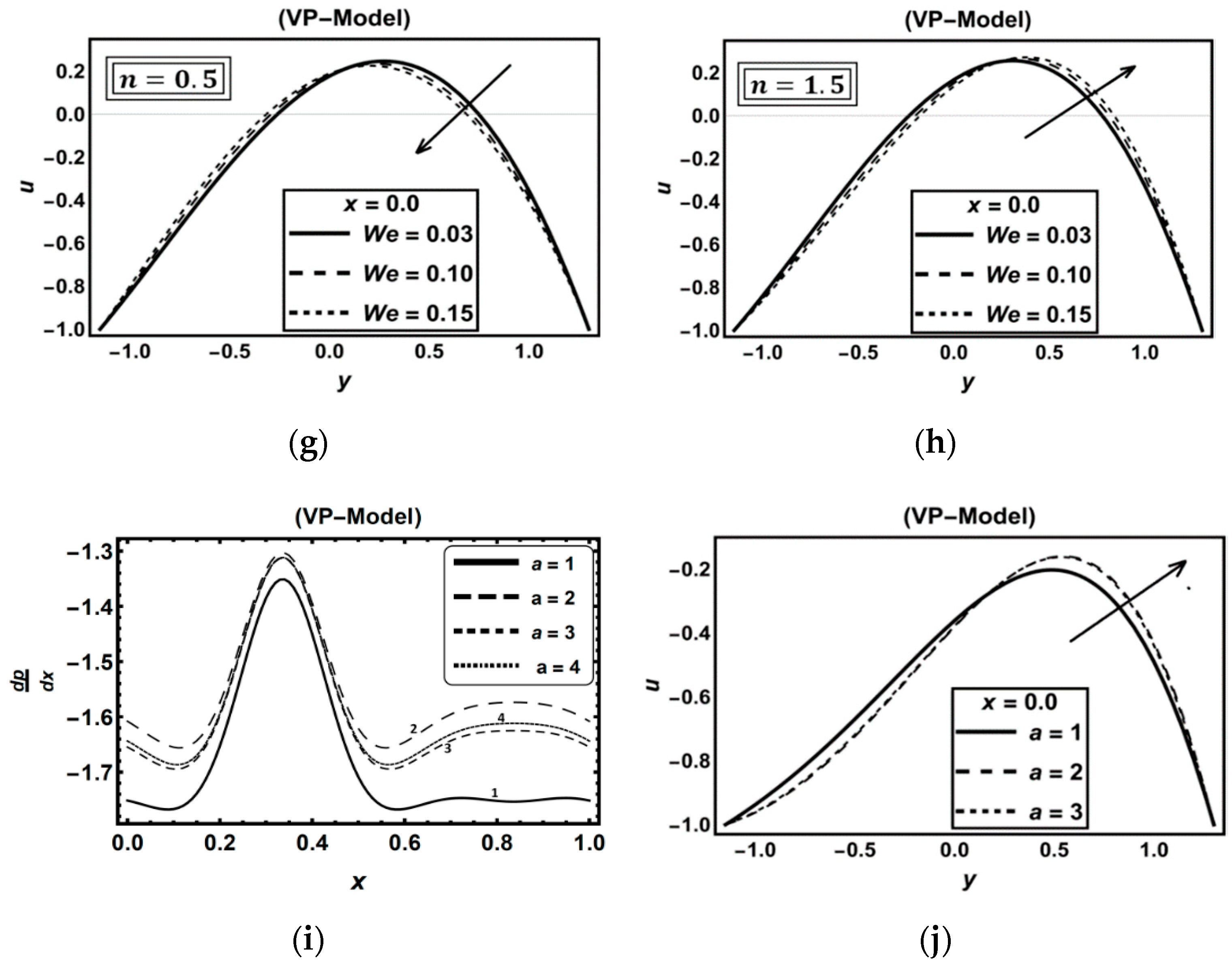
It is remarkable to observe that the impact of We on velocity in blood shear-thinning is quite the opposite of the case of blood shear-thickening.
(8)
Surprisingly, it is noticed that the pressure gradient starts showing an alternating increase/decrease behavior upon substituting positive constitutive integer values for the Carreau–Yasuda index parameter   a   ( a = 1 , 2 , 3 , ) . The maximum pressure gradient occurs for the case of the Carreau fluid   ( a = 2 ).
(9)
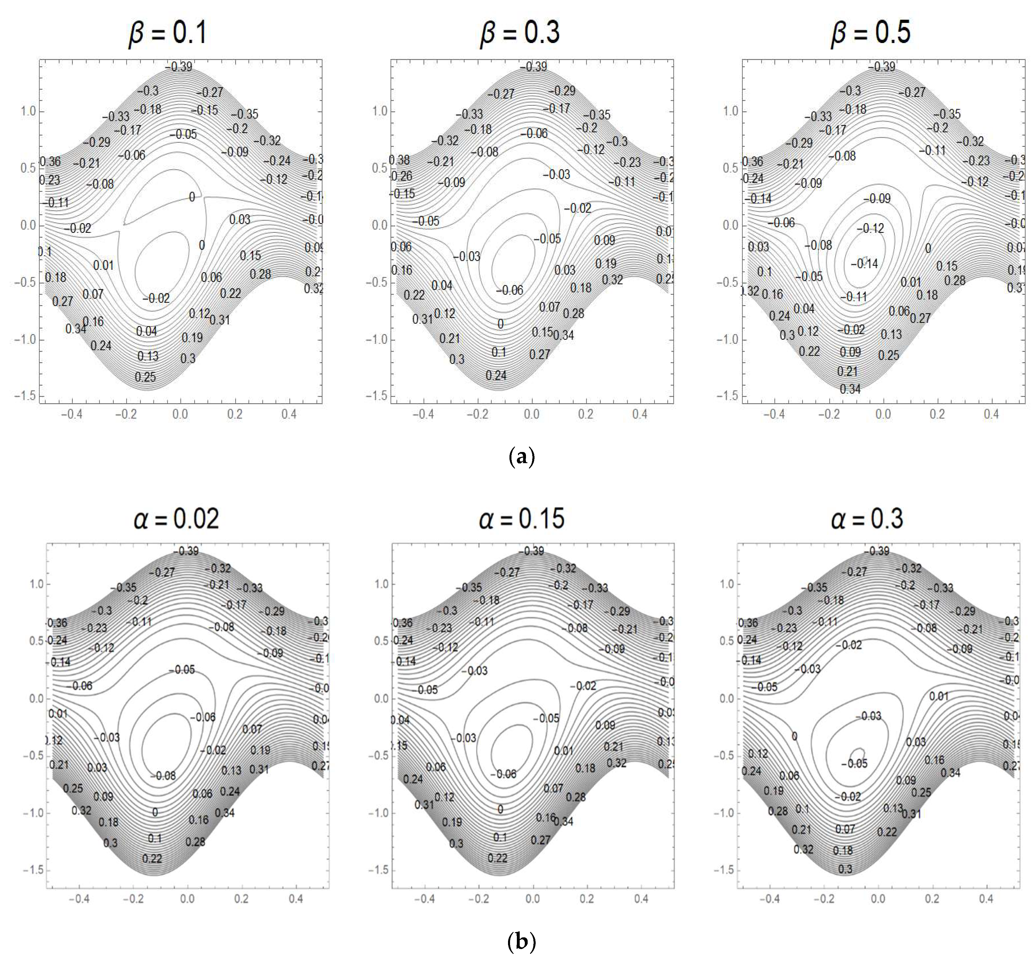
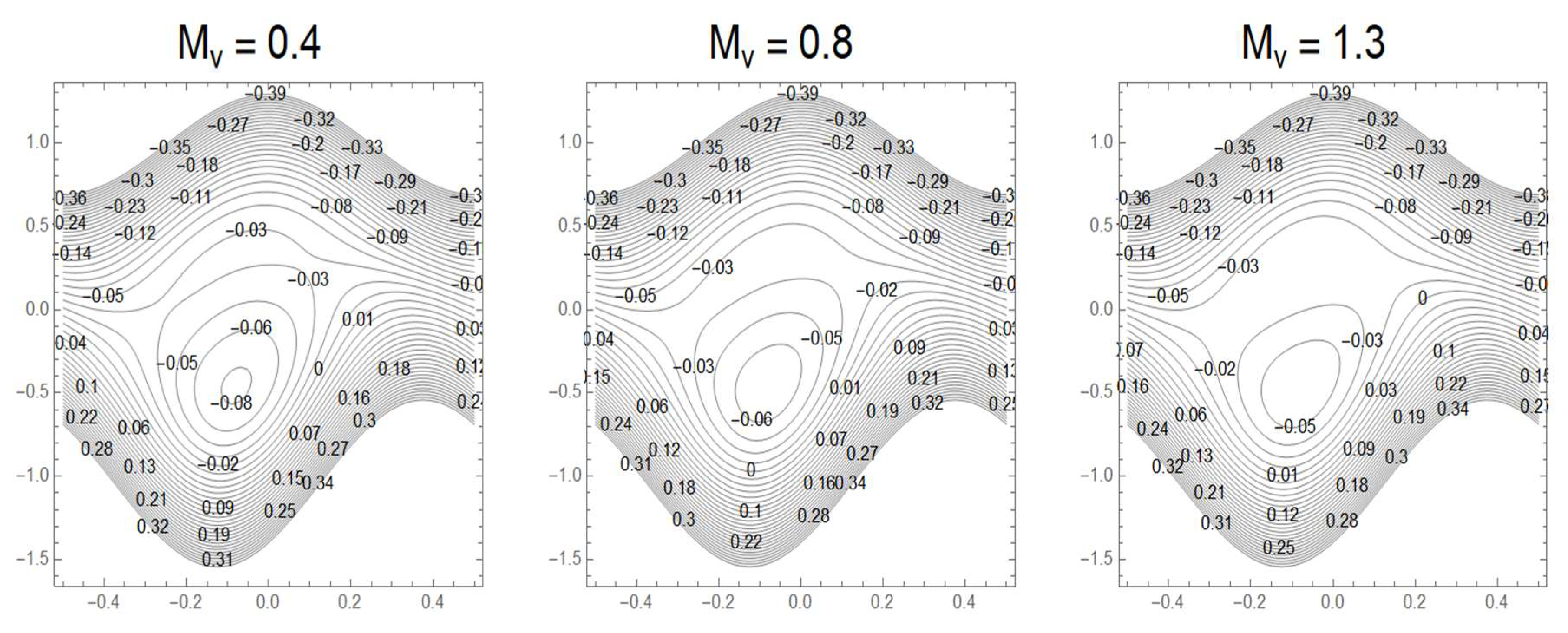
The number and size of the trapped bolus decreases with an increase in α and M v , while increasing with an increase of β .
In this study, we have adjusted a set of governing equations in physically sensible parameters. The work simulates how blood containing nanoparticles flow in microvessels in the presence of heat and mass transfer coupled with progressive patterns of microorganisms. The results delivered here are of fundamental interest in providing a theoretical basis to help improving human malignancy treatments by targeting anticancer drugs to the specific site of the tumor.

Author Contributions

Conceptualization, M.A.E. and K.S.M., methodology, M.A.E., software, M.A.E., validation, M.A.E. and K.S.M., formal analysis, M.A.E. and K.S.M., investigation, M.A.E. and K.S.M., writing—original draft preparation, M.A.E. and K.S.M., writing—review and editing, M.A.E. and K.S.M. All authors have read and agreed to the published version of the manuscript.

Funding

This research received no external funding.

Conflicts of Interest

The authors declare no conflict of interest.

References

  1. Nakhchi, M.E.; Hatami, M.; Rahmati, M. A numerical study on the effects of nanoparticles and their fins on performance improvement of phase change thermal energy storage. Energy 2021, 215, 119112. [Google Scholar]
  2. Nakhchi, M.E.; Esfahani, J.A. CFD approach for two-phase CuO nanofluid flow through heat exchangers enhanced by double perforated louvered strip insert. Powder Technol. 2020, 367, 877–888. [Google Scholar] [CrossRef]
  3. Nakhchi, M.E.; Rahmati, M.T. Entropy generation of turbulent Cu-water nanofluid flows inside thermal systems equipped with transverse-cut twisted turbulators. J. Therm. Anal. Calorim. 2019, 138, 1423–1436. [Google Scholar] [CrossRef]
  4. Ostwald, W. Ueber die rechnerische Darstellung des Strukturgebietes der Viskositat. Kolloid Z. 1929, 47, 176–187. [Google Scholar] [CrossRef]
  5. Carreau, P.J. Rheological equations from molecular network theories. Trans. Soc. Rheol. 1972, 16, 99–127. [Google Scholar] [CrossRef]
  6. Yasuda, K. Investigation of the Analogies between Viscometric and Linear Viscoelastic Properties of Polystyrene Fluids. Ph.D. Thesis, Massachusetts Institute of Technology, Cambridge, MA, USA, 1979. [Google Scholar]
  7. Nitesh, K.; Abdul-Khader, S.M.; Pai, B.R.; Kyriacou, P.A.; Khan, S.H.; Prakashinic, K. Computational fluid dynamic study on effect of Carreau-Yasuda and Newtonian blood viscosity models on hemodynamic parameters. J. Comput. Methods Sci. Eng. 2019, 19, 465–477. [Google Scholar]
  8. Gijsen, F.H.; van de Vosse, F.N.; Janssen, J.D. Wall shear stress in backward-facing step flow of a red blood cell suspension. Biorheology 1998, 35, 263–279. [Google Scholar]
  9. Alshare, A.; Tashtoush, B.; El-Khalil, H.H. Computational modeling of non-Newtonian blood flow through stenosed arteries in the presence of magnetic field. J. Biomech. Eng. 2011, 135, 114503. [Google Scholar] [CrossRef]
  10. Hong, H.; Song, J.M.; Yeom, E. Variations in pulsatile flow around stenosed microchannel depending on viscosity. PLoS ONE 2019, 14, e0210993. [Google Scholar] [CrossRef] [Green Version]
  11. Bernsdorf, J.; Wang, D. Non-Newtonian blood flow simulation in cerebral aneurysms. Comput. Math. Appl. 2009, 58, 1024–1029. [Google Scholar] [CrossRef] [Green Version]
  12. Hayat, T.; Abbasi, M.F.; Alsaedi, A.; Alsaedi, F. Hall and ohmic heating effects on the peristaltic transport of a carreau-yasuda fluid in an asymmetric channel. Z. Naturforsch. 2014, 69, 43–51. [Google Scholar] [CrossRef]
  13. Hayat, T.; Shafiquea, M.; Tanveera, A.; Alsaedi, A. Hall and ion slip effects on peristaltic flow of Jeffrey nanofluid with Joule heating. J. Magn. Magn. Mater. 2016, 407, 51–59. [Google Scholar] [CrossRef]
  14. Ramesh, K. Influence of heat and mass transfer on peristaltic flow of couple stress fluid through porous medium in the presence of inclined magnetic field in an asymmetric channel. J. Mol. Liq. 2016, 219, 256–271. [Google Scholar]
  15. Abbasi, F.M.; Hayat, T.; Alsaedi, A. Numerical analysis for MHD peristaltic transport of Carreau-Yasuda fluid in a curved channel with hall effects. J. Mol. Liq. 2015, 382, 104–110. [Google Scholar] [CrossRef]
  16. Eldabe, N.T.; Elogail, M.A.; Elshaboury, S.M.; Hasan, A.A. Hall effects on the peristaltic transport of Williamson fluid through a porous medium with heat and mass transfer. Appl. Math. Mod. 2016, 40, 315–328. [Google Scholar] [CrossRef]
  17. Hayat, T.; Farooq, S.; Alsaedi, A.; Ahmed, B. Hall and radial magnetic effects on radiative peristaltic flow of Carreau-Yasuda fluid in a channel with convective heat and mass transfer. J. Magn. Magn. Mater. 2016, 412, 207–216. [Google Scholar] [CrossRef]
  18. Bhatti, M.M.; Rashidi, M.M. Study of heat and mass transfer with Joule heating on magnetohydrodynamic (MHD) peristaltic blood flow under the influence of Hall effect. Propuls. Power Res. 2017, 6, 177–185. [Google Scholar] [CrossRef]
  19. Hayat, T.; Naseema, A.; Rafiq, M.; Alsaadi, F.E. Hall and Joule heating effects on peristaltic flow of Powell–Eyring liquid in an inclined symmetric channel. Results Phys. 2017, 7, 518–528. [Google Scholar]
  20. Ramesh, K.; Tripathi, D.; Beg, O.A.; Kadir, A. Slip and hall current effects on Jeffrey fluid suspension flow in a peristaltic hydromagnetic blood micropump. Iran. J. Sci. Technol. Trans. Mech. Eng. 2019, 43, 675–692. [Google Scholar] [CrossRef]
  21. Rafiq, M.; Yasmin, H.; Hayat, T.; Alsaadi, F. Effect of hall and ion-slip on the peristaltic transport of a nanofluid: A biomedical application. Chin. J. Phys. 2019, 60, 208–227. [Google Scholar] [CrossRef]
  22. Abdelsalam, S.I.; Bhatti, M.M. New insight into AuNP applications in Tumour treatment and cosmetics through wavy annuli at the nanoscale. Sci. Rep. 2019, 9, 260. [Google Scholar] [CrossRef] [PubMed]
  23. Hayat, T.; Abbasi, F.M.; Ahmed, B.; Alsaedi, A. Mhd mixed convection peristaltic flow with variable viscosity and thermal conductivity. Sains Malays. 2014, 43, 1583–1590. [Google Scholar]
  24. Hussain, Q.; Hayat, T.; Ashgar, S.; Ahmed, B.; Alsaadi, F. Heat and mass transfer analysis in variable viscosity peristaltic flow with hall current and ion-slip. J. Mech. Med. Biol. 2016, 16, 1650047. [Google Scholar]
  25. Alvi, N.; Latif, T.; Hussain, Q.; Asghar, S. Peristalsis of nonconstant viscosity Jeffrey fluid with nanoparticles. Results Phys. 2016, 6, 1109–1125. [Google Scholar] [CrossRef] [Green Version]
  26. Abbasi, F.M.; Hayat, T.; Ahmad, B. Hydromagnetic peristaltic transport of variable viscosity fluid with heat transfer and porous medium. Appl. Math. Inf. Sci. 2016, 10, 2173–2181. [Google Scholar] [CrossRef]
  27. Hayat, T.; Riaz, A.; Tanveer, A.; Alsaedi, A. Peristaltic transport of tangent hyperbolic fluid with variable viscosity. Therm. Sci. Eng. Prog. 2018, 6, 217–225. [Google Scholar] [CrossRef]
  28. Elogail, M.A.; Elshekhipy, A.A. Approximate analytical solutions to non-linear peristaltic flow with temperature-dependent viscosity parameters: Application of multi-step differential transform method (MsDTM). Can. J. Phys. 2018, 96, 287–299. [Google Scholar] [CrossRef]
  29. Ordal, G.W.; Goldman, D.J. Chemotactic repellents of Bacillus subtilis. J. Mol. Biol. 1976, 100, 103–108. [Google Scholar]
  30. Zhulin, I.B.; Bespalov, V.A.; Johnson, M.S.; Taylor, B.L. Oxygen taxis and proton motive force in Azospirillum brasilense. J. Bacteriol. 1996, 178, 5199–5204. [Google Scholar] [CrossRef] [Green Version]
  31. Shioi, J.; Dang, C.V.; Taylor, B.L. Oxygen attractant and repellent in Bacterial chemotaxis. J. Bacteriol. 1987, 169, 3118–3123. [Google Scholar] [CrossRef] [PubMed] [Green Version]
  32. Zhang, Z.; Li, Z.; Yu, W.; Li, K.; Xie, Z.; Shi, Z. Propulsion of liposomes using bacterial motors. Nanotechnology 2013, 24, 185103. [Google Scholar] [CrossRef] [PubMed] [Green Version]
  33. Martel, S. Swimming microorganisms acting as nanorobots versus artificial nanorobotic agents: A perspective view from an historical retrospective on the future of medical nanorobotics in the largest known three-dimensional biomicrofluidic networks. Biomicrofluidics 2016, 10, 021301. [Google Scholar] [CrossRef] [PubMed]
  34. Dogra, N.; Izadi, H.; Vanderlick, T. Micro-motors: A motile bacteria based system for liposome cargo transport. Sci. Rep. 2016, 6, 29369. [Google Scholar] [CrossRef] [PubMed] [Green Version]
  35. Felfoul, O.; Mohammadi, M.; Taherkhani, S.; Lanauze, D.; Zhong, X.Y.; Loghin, D.; Essa, S.; Jancik, S.; Houle, D.; Lafleur, M.; et al. Magneto-aerotactic bacteria deliver drug-containing nanoliposomes to tumour hypoxic regions. Nat. Nanotechnol. 2016, 11, 941–947. [Google Scholar] [CrossRef]
  36. Taktikos, J. Modeling the Random Walk and Chemotaxis of Bacteria: Aspects of Biofilm Formation. Doctoral Thesis, Technische Universität Berlin, Berlin, Germany, 2013. [Google Scholar]
  37. Charteris, N.; Khain, E. Modeling chemotaxis of adhesive cells: Stochastic lattice approach and continuum description. New. J. Phys. 2014, 16, 025002. [Google Scholar] [CrossRef] [Green Version]
  38. Hillen, T.; Painter, K.J. A user’s guide to PDE models for chemotaxis. J. Math. Biol. 2008, 58, 183–217. [Google Scholar] [CrossRef]
  39. Kuznetsov, A.V. Non-oscillatory and oscillatory nanofluid bio-thermal convection in a horizontal layer finite depth. Eur. J. Mech. B/Fluids 2011, 30, 156–165. [Google Scholar] [CrossRef]
  40. Amirsom, N.A.; Uddin, M.J.; Basir, M.F.; Kadir, A.; Bég, O.A.; Ismail, A.I. Computation of melting dissipative magnetohydrodynamic nanofluid bioconvection with second-order slip and variable thermophysical properties. Appl. Sci. 2019, 9, 2493. [Google Scholar] [CrossRef] [Green Version]
  41. Kim, Y.-C. Diffusivity of bacteria. Korean J. Chem. Eng. 1996, 13, 282–287. [Google Scholar]
  42. Hayat, T.; Aslam, N.; Khan, M.I.; Alsaedi, A. Mixed convective peristaltic flow of Carreau-Yasuda fluid in an inclined symmetric channel. Microsyst. Technol. 2019, 25, 609–620. [Google Scholar] [CrossRef]
  43. Eldabe, N.T.; Abo-Seida, O.M.; Abo-Seliem, A.A.; Elshekhipy, A.A.; Hegazy, N. Magnetohydrodynamic peristaltic flow of Williamson nanofluid with heat and mass transfer through a non-Darcy porous medium. Microsyst. Technol. 2018, 24, 3751–3776. [Google Scholar] [CrossRef]
  44. Eldabe, N.T.; Gabr, M.E.; Zaher, S.A. Two dimensional boundary layer flow with heat and mass transfer of magneto hydrodynamic non-Newtonian nanofluid through porous medium over a semi-infinite moving plate. Microsyst. Technol. 2018, 24, 2919–2928. [Google Scholar] [CrossRef]
  45. Mekheimer, Kh.S.; Zaher, A.Z.; Hasona, W.M. Entropy of AC electro-kinetics for blood mediated gold or copper nanoparticles as a drug agent for thermotherapy of oncology. Chin. J. Phys. 2020, 65, 123–138. [Google Scholar] [CrossRef]
  46. Kim, N.; Reddy, J.N. 3-D least-squares finite element analysis of flows of generalized Newtonian fluids. J. Nonnewton Fluid Mech. 2019, 266, 143–159. [Google Scholar] [CrossRef]
  47. Morrison, F.A. Understanding Rheology; Oxford University Press: New York, NY, USA, 2001; pp. 225–256. [Google Scholar]
  48. Miao, L.; Massoudi, M. Effects of shear dependent viscosity and variable thermal conductivity on the flow and heat transfer in a slurry. Energies 2015, 8, 11546–11574. [Google Scholar] [CrossRef] [Green Version]
  49. Elogail, M.A. Comments on “ ’combined effects of magnetohydrodynamic and temperature-dependent viscosity on peristaltic flow of Jeffrey nanofluid through a porous medium: Application to oil refinement’ by W.M. Hasona, A.A. El-Shekhipy and M.G. Ibrahim, International Journal of Heat and Mass Transfer, 2018, 126: 700–714”. Int. J. Heat Mass Transf. 2019, 128, 976–979. [Google Scholar]
  50. Mekheimer, Kh.S.; El-Kot, M.A. Influence of magnetic field and Hall currents on blood flow through a stenotic artery. Appl. Math. Mech. 2008, 29, 1093–1104. [Google Scholar] [CrossRef]
  51. Hayat, T.; Iqbal, R.; Tanveer, A.; Alsaedi, A. Mixed convective peristaltic transport of Carreau-Yasuda fluid in a tapered asymmetric channel. J. Mol. Liq. 2016, 223, 1100–1113. [Google Scholar] [CrossRef]
  52. Hayat, T.; Bilal, A.; Alsaedi, A.; Abbasi, F.M. Numerical study for peristalsis of Carreau-Yasuda nanomaterial with convective and zero mass flux condition. Results Phys. 2018, 8, 1168–1177. [Google Scholar]
  53. Khan, W.A.; Makinde, O.D. MHD nanofluid bioconvection due to gyrotactic microorganisms over a convectively heat stretching sheet. Int. J. Therm. Sci. 2014, 81, 118–124. [Google Scholar] [CrossRef]
  54. Kuznetsov, A.V. Nanofluid bioconvection in water-based suspensions containing nanoparticles and oxytactic microorganisms: Oscillatory instability. Nanoscale Res. Lett. 2011, 6, 100. [Google Scholar] [CrossRef] [PubMed] [Green Version]
  55. Buongiorno, J. Convective transport in nanofluids. J. Heat Trans. 2006, 128, 240–250. [Google Scholar] [CrossRef]
  56. Abd-elmaboud, Y.; Mekheimer, Kh.S.; Abdellateef, A.I. Thermal properties of couple-stress fluid flow in an asymmetric channel with peristalsis. J. Heat Trans. 2013, 135, 044502. [Google Scholar] [CrossRef]
  57. Demirel, Y. Nonequilibrium Thermodynamics, 3rd ed.; Elsevier: Amsterdam, The Netherlands, 2014; p. 82. [Google Scholar]
  58. Cengel, Y.A.; Cimbala, J.M.; Turner, R.H. Fundamentals of Thermal-Fluid Sciences, 5th ed.; Mc Graw Hill: New York, NY, USA, 2008; p. 428. [Google Scholar]
  59. Marini, C.P.; Russo, G.C.; Nathan, I.M.; Jurkiewicz, A.; McNiels, J. Effect of hematocrit on regional oxygen delivery and extraction in an adult respiratory distress syndrome animal model. Am. J. Surg. 2000, 180, 108–114. [Google Scholar] [CrossRef]
  60. Most, A.S.; Ruocco, N.A.; Gewirtz, H. Effect of a reduction in blood viscosity on maximal myocardial oxygen delivery distal to a moderate coronary stenosis. Circulation 1986, 74, 1085–1092. [Google Scholar] [CrossRef] [PubMed] [Green Version]
  61. Asha, S.K.; Sunitha, G. Effect of joule heating and MHD on peristaltic blood flow of Eyring–Powell nanofluid in a non-uniform channel. J. Taibah Univ. Sci. 2018, 13, 155–168. [Google Scholar] [CrossRef] [Green Version]
Figure 1. A schematic representation of blood in a microvessel containing microorganisms and nanoparticles.
Symmetry 12 02114 g001
Figure 2. ( a ) Influence of β on θ . ( b ) Influence of β on θ . ( c ) Influence of β on φ . ( d ) Influence of β on φ .
Symmetry 12 02114 g002
Figure 3. ( a ) Influence of ρ e v on Ω . ( b ) Influence of σ 1   on Ω . ( c ) Influence of λ 1 on Ω . ( d ) Influence of λ 1 on Ω . ( e ) Influence of λ 2 on Ω . ( f ) Influence of λ 2 on Ω . ( g ) Influence of R b v on θ . ( h ) Influence of   R b v on u .
Symmetry 12 02114 g003
Figure 4. ( a ) Influence of M v on θ . ( b ) Influence of M v on φ . ( c ) Influence of m on θ . ( d ) Influence of m   on φ . ( e ) Influence of M v on d p d x . ( f ) Influence of m on d p d x . ( g ) Influence of M v on Ω . ( h ) Influence of m on Ω . ( i ) Influence of M 0 on Ω .
Symmetry 12 02114 g004aSymmetry 12 02114 g004b
Figure 5. (a) Influence of M v on θ . (b) Influence of m on φ . (c) Influence of M v   on θ . (d) Influence of m on φ .
Symmetry 12 02114 g005aSymmetry 12 02114 g005b
Figure 6. ( a ) Influence of N t v on d p d x . ( b ) Influence of N t v on θ . ( c ) Influence of N t v on Ω . ( d ) Influence of N t v   on φ . ( e ) Influence of N b v on d p d x . ( f ) Influence of   N b v on Ω . ( g ) Influence of N b v on θ . (h) Influence of N b v on φ .
Symmetry 12 02114 g006aSymmetry 12 02114 g006b
Figure 7. ( a ) Influence of β on ξ . ( b ) Influence of β on ξ . ( c ) Influence of β on Ω . ( d ) Influence of β on φ . ( e ) Influence of α on Ω . ( f ) Influence of n on d p d x . ( g ) Influence of W e on u . ( h ) Influence of W e on u . ( i ) Influence of a on d p d x . ( j ) Influence of a on u .
Symmetry 12 02114 g007aSymmetry 12 02114 g007b
Figure 8. ( a ) Influence of   R n v on φ . (b) Influence of   R n v on θ . ( c ) Influence of   ϵ v   on φ . ( d ) Influence of ϵ v   on θ . ( e ) Influence of   G t v on   d p d x . ( f ) Influence of     G c v on d p d x . ( g ) Influence of   ϵ v on Ω . ( h ) Influence of   q on d p d x .
Symmetry 12 02114 g008
Figure 9. Streamline patterns for different values of   ( a )   β . ( b ) α . ( c ) M v .
Symmetry 12 02114 g009aSymmetry 12 02114 g009b
Table 1. The values of the embedded parameters for the CP-Model.
FigureDimensionless Constant Parameters
c b d ϕ   M 0 β ρ e 0 N b 0     N t 0   G c 0 G t 0 σ 1   R n 0 R b 0 E c   m α       a q P r 0     W e λ 1 λ 2 n   ϵ 0
Figure 2a0.30.51.1 π / 2 0.9-0.81.10.90.50.70.80.530.250.60.151 0.1 40.10.50.150.50.5
Figure 2c0.30.51.1 π / 2 0.9-0.81.10.90.50.60.60.510.250.60.251 0 40.150.30.10.50.2
Figure 4i0.30.51.1 π / 4 -0.350.81.20.50.50.50.70.520.250.50.251 0.1 30.150.50.150.50.8
Figure 7a0.30.51.1 π / 2 0.7-0.850.80.80.60.60.80.510.250.70.251 0 30.150.50.10.50.4
Table 2. The values of the embedded parameters for the VP-Model.
FigureDimensionless Variable Parameters
c b d ϕ   M v β ρ e v N b v     N t v   G c v G t v σ 1   R n v R b v E c   m α       a q P r v     W e λ 1 λ 2 n   ϵ v
Figure 2b0.30.51.1 π 2 0.9-0.81.10.90.50.70.80.530.250.60.151 0.1 40.10.50.150.50.5
Figure 2d0.30.51.1 π 2 0.9-0.81.10.90.50.60.60.510.250.60.251010.10.30.10.50.2
Figure 3a0.30.51.0 π 2 0.80.15-1.20.80.90.70.70.520.250.60.21 0.1 30.10.50.150.50.4
Figure 3b0.40.51.0   π 6 0.80.20.71.20.70.50.6-0.510.250.60.151 0.1 30.10.50.150.50.8
Figure 3c0.30.51.1   π 3 0.90.20.71.30.80.60.60.80.510.250.70.151 0.1 30.15-0.150.50.4
Figure 3d0.30.51.1   π 3 0.90.20.71.30.80.60.60.80.510.250.70.151 0.1 30.15-0.150.50.4
Figure 3e0.30.51.1       π 2 0.90.20.71.30.80.60.60.80.510.250.70.151   0.1 . 30.150.5-0.50.4
Figure 3f0.30.51.1 π 2 0.90.2071.30.80.60.60.80.510.250.70.151 0.1 30.150.5-0.50.4
Figure 3g0.30.51.1 π 3 0.80.40.71.20.90.70.70.50.5-0.250.60.151 0.1 40.150.50.150.50.8
Figure 3h0.30.51.1 π 2 0.80.30.91.20.60.70.80.60.5-0.250.70.151 0.1 30.150.50.150.50.4
Figure 4a0.30.51.1 π 2 -0.250.91.10.70.60.60.80.510.250.70.21 0.1 30.150.50.150.50.5
Figure 4b0.40.51.1 π 2 -0.250.91.10.70.60.60.80.510.250.70.21 0.1 30.150.50.150.50.2
Figure 4c0.30.51.1 π 2 0.90.250.91.10.70.60.60.80.510.25-0.21 0.1 30.150.50.150.50.2
Figure 4d0.40.51.1 π 2 0.90.250.91.10.70.60.60.80.510.25-0.21   0.1 . 30.150.50.150.50.2
Figure 4e0.40.71.1       π 6 -0.30.71.20.70.70.80.70.510.250.90.251 1.3 30.150.50.120.50.5
Figure 4f0.40.71.1       π 6 0.60.30.71.20.80.70.80.70.530.25-0.251 1.3 30.150.50.150.50.5
Figure 4g0.30.51.1       π 4 -0.350.81.20.50.50.50.70.520.250.50.251   0.1   40.150.50.150.50.8
Figure 4h0.40.51.1 π 4 0.90.350.81.20.50.60.50.70.520.25-0.251 π 6 40.150.50.150.50.8
Figure 5a0.30.51.1 π 6 -0.40.61.41.10.90.50.70.540.2510.21 0.1 50.150.50.150.50.2
Figure 5b0.30.51.1 π 6 1.10.450.61.40.90.81.40.70.540.25-0.21 0.1 50.150.50.150.50.2
Figure 5c0.30.51.1 π 6 -0.40.51.40.90.81.10.60.540.30.60.21     0.1 50.150.50.150.50.2
Figure 5d0.30.41.1       π 2 1.30.30.60.90.80.81.40.60.510.3-0.21   0.1 50.10.50.150.50.2
Figure 6a0.30.51       π 12 0.80.30.71.2-0.70.50.70.540.250.70.251 1.3 40.150.50.10.50.2
Figure 6b0.30.41.1       π 4           0.90.40.71.4-0.50.50.70.510.250.70.251 0.1 30.150.40.10.50.5
Figure 6c0.40.51.1       π 2           0.90.350.81.1-0.60.60.70.510.250.70.251 0.1 30.150.50.150.50.4
Figure 6d0.40.51.1       π 3           0.90.40.71.3-0.50.50.70.510.250.70.251 0.1 30.150.40.120.50.5
Figure 6e0.30.51     π 2 0.80.30.7-0.70.80.50.80.540.250.70.251 1.3 40.150.50.150.50.5
Figure 6f0.30.50.9     π 6 0.60.40.8-10.80.70.70.510.250.60.251 0.1 30.150.50.150.50.4
Figure 6g0.30.51.1     π 2 0.90.350.8-10.80.60.60.510.250.50.251 0.1 30.150.50.150.50.4
Figure 6h0.30.50.9     π 3 0.70.30.7-0.60.50.50.70.510.250.80.251 0.1 30.150.40.120.50.5
Figure 7b0.30.41.1     π 2   0.7-0.851.30.80.60.60.80.510.250.70.251030.150.50.10.50.4
Figure 7c0.30.51.1     π 3 0.9-0.81.30.70.70.90.80.520.250.60.21 0.1   40.15--0.50.5
Figure 7d0.30.51.1     π 3 0.9-0.81.30.70.70.90.80.520.250.60.21 0.1   40.15--0.50.5
Figure 7e0.40.61.1     π 2   0.80.2511.20.70.60.70.50.520.250.6-1 0.1   40.10.50.10.50.25
Figure 7f0.30.50.9 π 4   0.80.40.71.30.60.70.80.50.510.250.60.21 1.1   40.150.50.15-0.4
Figure 7g0.30.50.9 π 3   0.70.30.71.10.70.60.80.70.530.250.80.21 0.5   3-0.50.15-0.4
Figure 7h0.30.50.9 π 3   0.70.30.71.10.70.60.80.70.530.250.60.21 0.5   3-0.50.15-0.4
Figure 7i0.30.51 π 2   0.90.30.71.30.80.71.20.70.520.250.70.2- 1.2 40.30.50.120.50.5
Figure 7j0.30.50.9 π 3   0.80.411.10.70.60.80.70.540.2510.25- 1.3 30.10.50.150.50.6
Figure 8a0.30.51.1 π 4   0.80.30.81.10.80.60.70.7-30.250.70.21 0.1 30.150.50.150.50.4
Figure 8b0.30.50.9 π 4   0.80.40.81.10.70.60.70.7-30.250.70.251 0.1 30.10.50.150.50.4
Figure 8c0.30.51.1         π 2   0.80.250.71.20.70.80.80.70.510.250.60.151 0.1 30.150.50.120.5-
Figure 8d0.30.51.1         π 2   0.80.250.71.20.70.80.80.80.510.250.60.151 0.1 30.150.50.120.5-
Figure 8e0.30.51.1       π 12 0.80.40.81.20.60.7-0.70.510.20.60.251 1.3 30.150.50.150.50.5
Figure 8f0.30.51.1       π 12 0.80.40.81.10.6-0.70.70.510.250.60.251 1.3 30.10.50.150.50.5
Figure 8g0.30.51.1       π 2 0.50.60.610.90.60.70.90.550.250.60.151 0.2 40.150.50.150.5-
Figure 8h0.30.51.100.80.40.810.60.50.70.70.510.250.60.251-40.10.50.150.50.5
Figure 9a0.40.51.1     π 4 0.8-0.810.50.80.80.70.510.250.70.151 0.2 40.150.50.150.5-
Figure 9b0.30.51.1     π 4 0.80.30.81.20.50.80.80.70.510.250.7-1 0.2 40.150.50.150.50.5
Figure 9c0.30.51.1     π 4 -0.30.81.20.50.80.80.70.510.250.70.151 0.2 40.150.50.150.50.5
Publisher’s Note: MDPI stays neutral with regard to jurisdictional claims in published maps and institutional affiliations.

