Extending the Fully Bayesian Unfolding with Regularization Using a Combined Sampling Method


Joint Laboratory of Optics of Palacký University and Institute of Physics AS CR, Faculty of Science, Palacký University, 17. listopadu 12, 771 46 Olomouc, Czech Republic
*
Author to whom correspondence should be addressed.
†
These authors contributed equally to this work.
Symmetry 2020, 12(12), 2100; https://doi.org/10.3390/sym12122100
Submission received: 13 November 2020
/
Revised: 11 December 2020
/
Accepted: 15 December 2020
/
Published: 17 December 2020
(This article belongs to the Special Issue Particle Physics and Symmetry)
Abstract
:Regularization extensions to the Fully Bayesian Unfolding are implemented and studied with an algorithm of combined sampling to find, in a reasonable computational time, an optimal value of the regularization strength parameter in order to obtain an unfolded result of a desired property, like smoothness. Three regularization conditions using the curvature, entropy and derivatives are applied, as a model example, to several simulated spectra of top-pair quark pairs that are produced in high energy collisions. The existence of a minimum of a between the unfolded and particle-level spectra is discussed, with recommendations on the checks and validity of the usage of the regularization feature in Fully Bayesian Unfolding (FBU).
1. Introduction
This study is motivated by unstable results of unfolding in the case of spectra with a large number of bins or with a poorly diagonal migration matrix. In order to obtain the expected smooth results, a bias is carefully introduced via a regularization function. We focused on the Fully Bayesian Unfolding (FBU) method [1].
Other unfolding methods than FBU have already been introduced, including regularization features. Because FBU has the ability to provide the full probability posterior of the result and thus stands out from other methods, it is interesting to also provide FBU with the regularization option.
This study uses several over-binned spectra, so the unfolding without regularization results in fluctuating, high-variance unfolded spectra. These were constructed by fine binning, so that the migration matrix is under-represented on diagonal. Five typical spectra considering the production of top quark pairs in collisions were chosen, namely the pseudorapidity and transverse momentum of the hadronicaly decaying top quark, and pseudorapidity , transverse momentum , and mass of the system.
The regularization feature was introduced as a prior in the likelihood. However, the problem which remains is how strongly should user apply the regularization to get the optimal unfolded spectrum, which should be close to the particle spectrum, but, at the same time, respects the desired regularization property, e.g., low curvature. The power of regularization is governed by the regularization strength parameter . The higher the , the stronger the regularization.
An algorithm for finding the optimal value of in a reasonable time via a combined sampling is given so that the best unfolding result is achieved, representing the main message of this paper.
2. Unfolding
The unfolding procedure corrects measured spectra for the resolution, efficiency, and acceptance effects of the detector usually to the particle level. The principles of the Fully Bayesian Unfolding method are based on the Bayes theorem
where the conditional probability reads the probability of A, given as B. Fully Bayesian Unfolding provides the full probability posterior of the result, which gives extra information when compared to other unfolding methods [2]. Rewriting Equation (1), the probability of the truth spectrum , given the data , is
where the is a normalization factor, is the likelihood function, and is a prior probability density for . In the case of the algorithm is non-regularized. By inserting an arbitrary regularization function instead of , one can intentionally bias the final result towards a suitable property, e.g., to be smooth, and unfolding is then called regularized. The convenient way is to use an exponential function with regularization strength parameter and an inner function
If the parameter , the prior , and no regularization is applied; on the other hand, the higher value of , the more dominant the regularization term.
2.1. Simulated Spectra
The input pseudo-data spectrum is simulated for the process at while using MadGraph5 [3] software, Pythia8 generator [4], and Delphes [5] detector simulation with an ATLAS card while using basic kinematics cuts in order to obtain a realistic sample of top quark pairs decaying in a semi-leptonic way , with more details being described in [6].
2.2. Defining Equations of Unfolding
The necessary ingredients for unfolding are the data spectrum and the migration matrix M, which is normalized, so that it maps the probability of an event at the truth (particle) level bin i to be reconstructed (measured) at the detector level bin j.
The schematic formula describing unfolding for the case of a simple migration matrix inversion is
In this paper, the background spectrum is not taken into account. The efficiency and acceptance corrections are derived from projections of the migration matrix M divided by the simulated particle level or data spectrum , as
Because our data are simulated we set = and Equation (4) becomes
The production of spectra was divided into two statistically independent sets A and B, where set A is used for unfolding components and set B is taken as pseudo data input to unfolding
The result of unfolding is compared to the corresponding particle level spectrum (green line in Figure 1a). The test between the unfolded and particle spectrum divided by the number of degrees of freedom (number of the bins), , is calculated in the standard way, as follows
The input components that are needed for the unfolding process are visualized for the case of the spectrum presented in Figure 1.
In essence, the FBU unfolding technique exploits the response matrix to fold a probe truth-level spectrum, obtaining the detector-level spectrum, and computing a likelihood between such folded spectrum and the actual data. This elegantly avoids issues of singularities in explicit matrix inversion or their regularization, as e.g., in the SVD technique [7]. The tricky part of the FBU is how to effectively sample the truth space in the region giving large likelihood values.
2.3. Likelihood Function
The likelihood function is given by the product of Poisson distributions in case of counts as
where
and
After unfolding, the probability is divided by the efficiency correction . The acceptance correction that is shown in Figure 1b takes on values [0,1] and, thus, the factorial is computed using the Gamma function as
In the simplified case of no background (), pseudo data , and introducing the natural logarithm, since the sampling of the functions is more numerically stable, Equation (9) becomes
which can be rewritten as
This expression has the advantage of allowing one to find the maximum of by sampling the log-likelihood function and the regularization function separately and tune the regularization parameter , so that the optimal can be found in a much shorter time than sampling the full likelihood for every possible value of .
In this study, both of the approaches were used: the one when sampling was applied to the function as a whole, denoted as full sampling, and the one when sampling of the two components and is performed separately, denoted as combined (fast) sampling. These methods will be described in detail in Section 2.6.
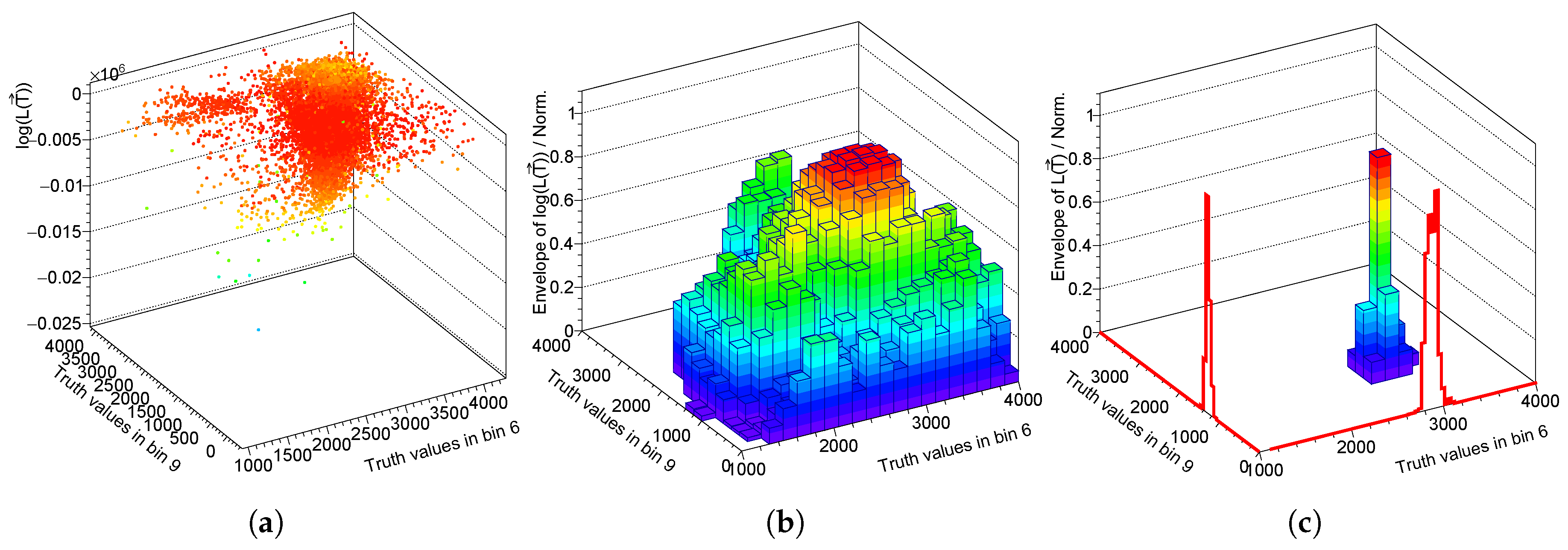
Figure 2a shows an example of the log-likelihood, sampling of the function for the spectrum and its projection to the and bin . Figure 2b is created while using the highest points of the and, thus, represents an envelope of the , while Figure 2c represents the exponential of the envelope of the original , with the posteriors plotted along the x and y axes (red lines), which are the marginalized binned probability densities that are analytically given as
The mean and standard deviation of the posteriors are taken as the unfolded result in each bin in this study in order to construct the unfolded spectrum and its statistical uncertainty. Another approach is to fit the posteriors and use parameters from the fit, see Figure 3, but this method is not used in this paper, since the regularization can change the shape of the posterior to non-Gaussian.
The advantage of the FBU in comparison to other unfolding methods is in providing the whole probability distribution. Marginalizing this probability to one-dimensional posteriors the user gains the probability distribution of the unfolded result for each bin and it can decide a custom statistical property to define the unfolding result and its uncertainty in the particular bin while other methods usually provide only a single number with some uncertainty. Thus, FBU provides more user control over the unfolded output interpretation. Furthermore, marginalizing the whole probability into two dimensions enables one to study cross-bin correlations, accessible only via dedicated pseudo experiments in other methods. Another advantage is the possibility of a natural inclusion of systematic uncertainties variation by introducing prior distributions for corresponding nuisance parameters directly into the likelihood function and performing a simultaneous fit, which is a procedure known as profiling.
2.4. Motivation for the Regularization
Figure 4 illustrates the unfolding process and proceeds from the (blue) pseudo data line to the (red) unfolded line in Figure 4a, which fluctuates due to low occupied diagonal of the migration matrix M (Figure 1c). One can improve the variance of the result by introducing a regularization term aiming to diminish the curvature of the unfolding result (Figure 4b) with the optimal strength parameter derived using the full sampling algorithm discussed in Section 2.3 (Figure 5), so that the resulting between particle and unfolded spectra is minimal.
On the other hand, if one sets the strength of regularization to a very large number, e.g., , the corresponding is high and the unfolded result departs from the particle level spectrum, see Figure 4c.
This implies that may have a minimum as function of (see Figure 5) and the aim of this study is to provide a way to find such a minimum in a reasonable computational time. In the next section, we describe three regularization functions used in this study.
2.5. Regularization Functions
While the regularization function can be taken as any arbitrary function, we motivate several choices [1]. The aim of the negative entropy, curvature and derivatives is to smoothen the unfolded spectra.
- Entropy regularization
- Curvature regularizationwhere
- First derivative regularizationwhereand N is the number of bins, is the width of tth bin, and is the bin center of the tth bin.
Each of the regularization functions has a different effect on the full likelihood, see Figure 6. While sampling the likelihood according to gradient of , i.e., leaving for the moment, the values of are stored.
2.6. Sampling the Likelihood Function
Effective sampling plays a crucial role in finding extremes of the likelihood function. In this paper, a private implementation of the Markov chain Hamiltonian Monte Carlo [8] method is used when each point of a function is derived from the previous point, thus forming a chain. The problem of finding the maximum of the likelihood function is transformed to generate a sample via the study of motion of a virtual particle in the potential represented by the likelihood function in an N-dimensional space.
The Hamiltonian of a particle with momentum in potential , depending on position vector , can be reformulated from the classical expression
to the studied problem, where the position vector is substituted by the vector of particle-level truth values and the potential by the negative log-likelihood function , so that
The first Hamiltonian equation of motion
becomes in the space of truth values and momentum
and numerically
where is the time interval. Each point in momentum space is updated as
Similarly, the second equation of motion
becomes
so the truth (position) value is updated in time, according to
and the momentum as
Equations (26), (29) and (30) provide one and two-step updates for and , respectively. The time interval is adapted in first few steps and it then stays constant for the rest of the sampling. The initial momentum is chosen randomly according to normal distribution and the initial truth vector is randomly chosen while using uniform distribution within limits set by user or using a default expected range in i-th bin . These limits create a hyper-cube, in which the sampling is performed. The algorithm details are described in [8].
The introduction of the canonical momentum and shifting the N dimensional problem to dimensions is one of the key features of the Hamiltonian MC chain generator. Classical mechanics Hamiltonian equations of motions are then employed, with the negative likelihood playing the role of a potential for a particle moving in the generalized phase-space, under the conservation of the total energy. The invariance of the system w.r.t. time translations is the motivation for exploring the trajectory of such a particle for different initial conditions, which leads to effectively sampling a larger phase space and more of the classical trajectories, thus increasing the probability of reaching the global minimum of the potential, i.e., the likelihood maximum.
3. Regularization
This section provides an overview of unfolding characteristics as function of the regularization strength parameter . Throughout this paper, the original parameter is normalized while using the number of bins N and the curvature, entropy, or derivatives of the particle spectrum that are generally symbolized by as
and, in the dependence, figures are used, so different spectra and regularization functions acquire similar values of , which are then more comparable.
3.1. Evolution of Posteriors with
Two effects come into shaping the posteriors with stronger regularization applied. First is the shifting of the peak, which is welcome in obtaining the expected modified unfolded spectrum. The second effect decreases the posteriors width and this effect decreases the uncertainty in the mean for each bin sometimes down to an artificially infinitesimal small width with extremely high and, thus, undesirably somewhat increases the when comparing unfolded and truth spectra.
Because these are two competing effects, a minimum of the may or may not appear. Figure 7 shows the posterior in the 15th bin of the spectrum for three scenarios. First, when no regularization is applied, so , then with regularization with optimal , so the final is the smallest, and finally with an extremely high when the posterior becomes almost a Dirac -function.
3.2. Evolution of Curvature, Entropy, and Derivatives with
One of the first checks whether the regularization works properly is to study the curvature, entropy and derivatives of the unfolded spectra with respect to the increasing regularization strength . The expected result is that, with higher , the curvature decreases and the unfolded spectrum is smoother. The same characteristics also holds for entropy and derivatives. Figure 8 shows the decrease of curvature, entropy, and derivatives with increasing , as expected.
3.3. Evolution of Bin Cross-Correlations with
Using the likelihood projection to two different bins, the cross-bin correlations can be derived. Figure 9 shows the overall matrix built from these correlation factors. While, in case of (a) (), the bin correlations are minimal, the progressing trend in case (b) (), and finally (c) () is evident. Thus, the stronger regularization is the more bins of the unfolded spectrum are correlated between each other.
In order to quantify the increase of correlations, the averaged sum of off-diagonal elements of bin correlation matrix A is shown for various , given by
and also its absolute value version to study the sum of correlations and anti-correlations
These bin-averaged cross correlations and are shown in Figure 10, and the increasing trend proves that, the stronger regularization, the more correlated the unfolding result over bins.
3.4. Evolution of and Bin Uncertainties with
The is calculated as
where each for one particular bin is taken as the mean of the posterior and the uncertainty as the standard deviation of the posterior. Because the width of the posterior is observed to decrease with rising , the also has to rise. In order to naively separate effects of spectra smoothing and posteriors narrowing, two variables and were studied, being defined as
and shown in Figure 11 and Figure 12.
If the effects of shifting and narrowing the posterior are independent then and ratio should be comparable
which can be seen in Figure 13.
The problem of finding the optimal by finding the minimal is the time that is needed to create such a graph as in Figure 13, while each point of the graph is obtained by running the full unfolding. In the next section, an algorithm is described, which enables one to estimate the minimum of in a much faster way.
4. Combined Sampling as a Faster Algorithm
In order to speed up the algorithm which estimates the minimum value, the algorithm of combined sampling is proposed. The main idea is to sample separately the function and the regularization function and then vary the parameter to obtain the overall likelihood
A problem arises with sampling the regularization function since this function is not smooth and sampling algorithm can end up mapping only the local minima. To avoid this is, an auxiliary function
is sampled, where so the global minimum is dominated by . The function stands in sampling only for the purpose of providing a correct gradient, while values of and are stored separately, so post-unfolding these values can be used to compute in a fast way the full desired posterior of
for any .
This faster combined sampling approach is shown in blue in Figure 14, while the red points stand for the full sampling, where, for each point in , a new sampling had to be performed. Figure 14 shows a very good agreement between combined and full sampling methods in terms of their minima. In the case of derivative regularization in Figure 14c the full sampling method (red) does not cover the highest values of in the range of approximately [, ]. The reason is that the regularization function of derivatives, as compared to the curvature and entropy, is very narrow, approaching for high almost a -function, see Figure 6c and, thus, the sampling either takes infinite time to find such a peak in the wide domain of the function or is stopped by reaching the maximum number of iterations and the resulting is very high as the global maximum is not found.
5. Accidental Minima of
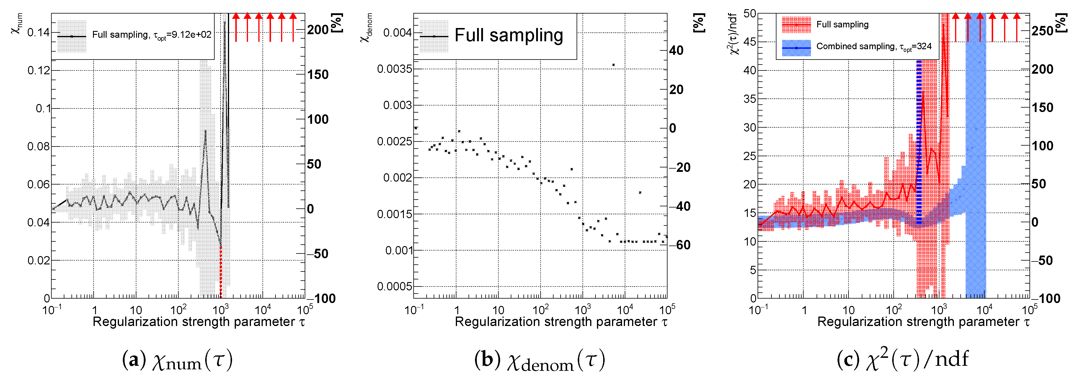
In the case of unfolding without regularization being effective enough so no smoothing is actually needed, the narrowing of posteriors can cause an accidental minimum in the function. The example of the spectrum shows the variable as a flat function with increasing tail in high values, see Figure 15a. At the same time, the decreases rapidly and the ratio of these components as well as exhibit a minimum at solely due to the narrowing of posteriors.
This accidental minimum does not improve the smoothness of the spectrum, as illustrated in Figure 16. The unfolded spectrum while using regularization in Figure 16b only decreases the uncertainties (red line) when compared to Figure 16a while not providing a smoother spectrum, as can be seen in the ratio and only a minor decrease of .
The regularization is not effective due to the fact that the tail of the spectrum has lower number of events compared to the first half of the spectrum. The contribution to the curvature is thus small in the tail. The solution would be to switch on the regularization only for the second half of the spectrum as shown in Figure 16c where computed in the tail region of the spectrum decreases when compared to Figure 16a,b, also affecting the full via a change of the global maximum of the full likelihood.
6. Hidden Minima of
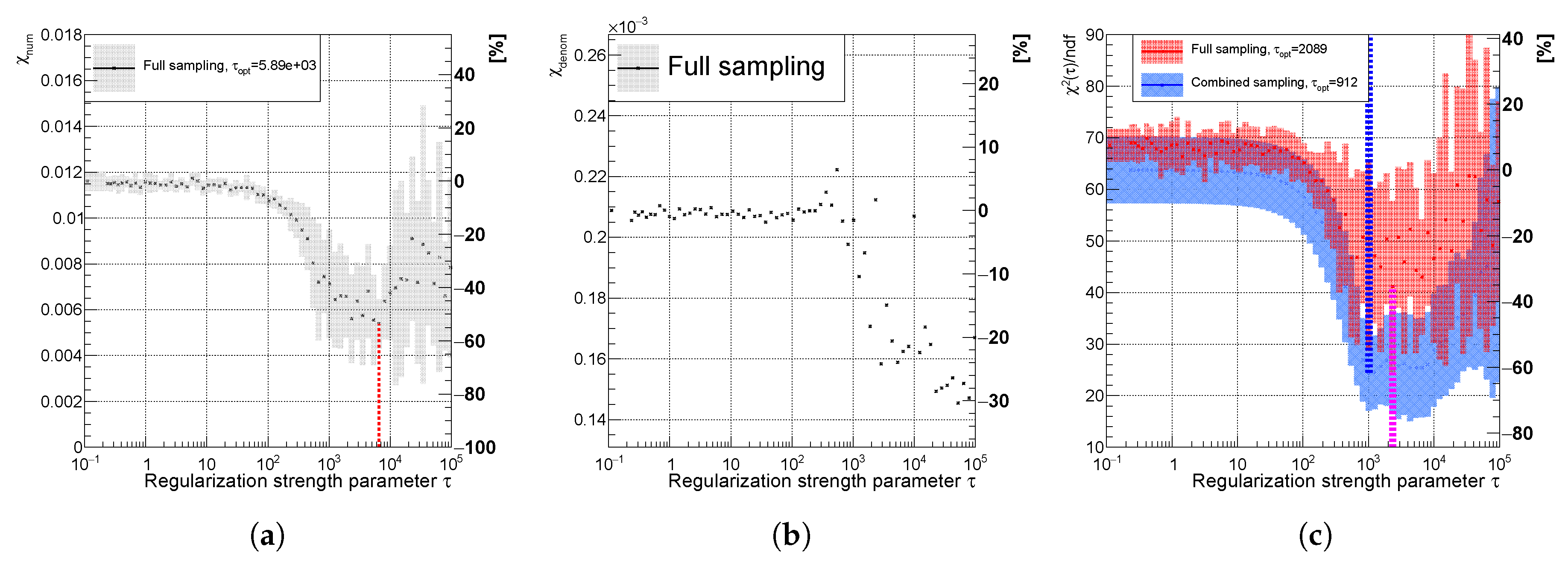
If the smoothing effect that is expressed by in Figure 17a has a minimum and if the narrowing effect described by in Figure 17b starts to decrease with a similar or sharper slope than (), then the real minimum in in Figure 17c vanishes and flattens, so finding the optimal for the spectrum in Figure 18 cannot be identified by minimizing as a function of . Figure 18b shows the improved unfolded spectrum that was obtained while using the minimum of . However, due to the narrowing of posteriors, the increases as compared to Figure 18a (no regularization).
7. Real Minima of
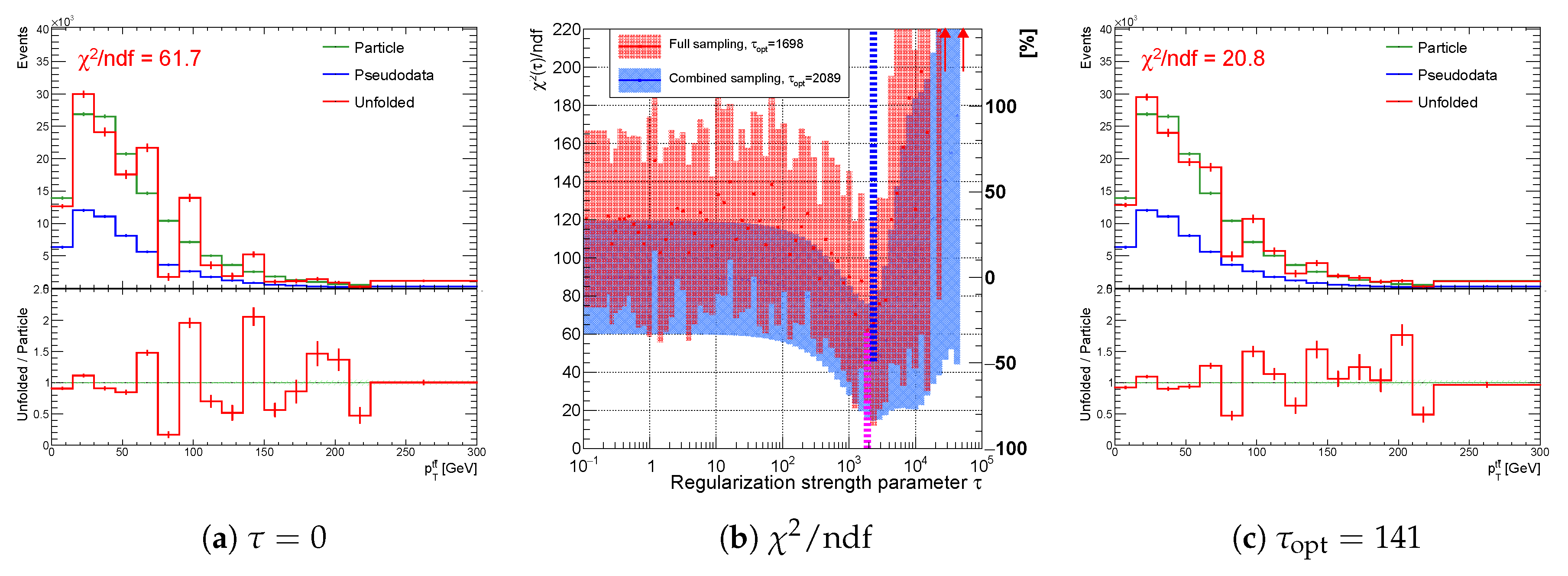
If the smoothing effect expressed by in Figure 19a has a global minimum and, if the narrowing effect described by in Figure 19b starts to decrease around the same region of values as (), then a real minimum in in Figure 19c is observed and it helps to improve the desired property the unfolded spectrum, as shown for the spectrum of in Figure 20.
8. Results
The results for the spectra of , and were already shown in Figure 16, Figure 18 and Figure 20. In this section, remaining two studied spectra and are shown in Figure 21 and Figure 22, where, for , the regularization is unnecessary.
The results of all five spectra and their characteristics are summarized in Table 1, Table 2 and Table 3 in order to attempt finding a common feature that could predict the existence of real minima. Firstly, a characteristic of the migration matrix M was studied defined as
where has the meaning of averaged diagonal elements. As a second characteristic, the correlation factor is computed while using the ROOT’s TH2D class and the GetCorrelationFactor() method [9].
Another characteristic that is shown in the Table 2 corresponds to the shape of the unfolded spectra. The curvature , entropy and derivatives of unfolded spectra without regularization are given relative to the curvature , entropy , and derivatives of the truth particle spectra.
9. Discussion
We studied a method of finding an optimal regularization strength parameter and developed an independent implementation of two methods of adding regularization terms to the Fully Bayesian Unfolding and proposing a fast combined sampling method for finding an optimal value of the regularization strength parameter . The C++ version of the Fully Bayesian Unfolding was implemented into a private modification to RooUnfold [10], which is a widely used unfolding package in HEP.
The recommended option for the user is to use the combined sampling algorithm, which returns the curve in a shorter time than the regular full sampling method, see Table 3.
The time that is needed to produce curve while using the full sampling depends on the number of points in the user wishes to obtain (here, 67 points × three methods), while, using the combined method, the sampling algorithm is only run four times: first, to sample the log-likelihood function without the regularization part and afterwords three times for each of the regularization functions (curvature, entropy, and derivative), which roughly explains the time-saving ratio 4:(3×67) .
While no clear relation between the spectra characteristics in Table 1 and Table 2 and real minima of was observed, the user is encouraged to evaluate , , and him/herself in order to convince oneself of the validity and usefulness of the regularization.
While we provided an example for the spectra of reconstructed top quarks that are produced in collisions, the applicability of the method is not at all unique to spectra in high energy physics. Any inverse problem with finite migrations and a large number of bins is a potential candidate for benefitting from the fast sampling regularization that is introduced for the FBU method.
Author Contributions
Both authors contributed equally to this work. Both authors have read and agreed to the published version of the manuscript.
Funding
This research received no external funding.
Acknowledgments
The authors gratefully acknowledge the support from the project of the Czech Science Foundation project GAČR 19-21484S as well as the support from the project IGA_PrF_2020_007 of the Palacky University.
Conflicts of Interest
The authors declare no conflict of interest.
References
- Choudalakis, G. Fully Bayesian Unfolding. arXiv 2012, arXiv:1201.4612. [Google Scholar]
- Prosper, H.B.; Lyons, L. PHYSTAT 2011 Workshop on Statistical Issues Related to Discovery Claims in Search Experiments and Unfolding; CERN: Geneva, Switzerland, 2011. [Google Scholar] [CrossRef]
- Alwall, J.; Frederix, R.; Frixione, S.; Hirschi, V.; Maltoni, F.; Mattelaer, O.; Shao, H.S.; Stelzer, T.; Torrielli, P.; Zaro, M. The automated computation of tree-level and next-to-leading order differential cross-sections, and their matching to parton shower simulations. J. High Energy Phys. 2014, 2014, 79. [Google Scholar] [CrossRef] [Green Version]
- Sjöstrand, T.; Ask, S.; Christiansen, J.R.; Corke, R.; Desai, N.; Ilten, P.; Mrenna, S.; Prestel, S.; Rasmussen, C.O.; Skands, P.Z. An Introduction to PYTHIA 8.2. Comput. Phys. Commun. 2015, 191, 159–177. [Google Scholar] [CrossRef] [Green Version]
- De Favereau, J.; Delaere, C.; Demin, P.; Giammanco, A.; Lemaitre, V.; Mertens, A.; Selvaggi, M.; DELPHES 3 Collaboration. DELPHES 3: A modular framework for fast simulation of a generic collider experiment. J. High Energy Phys. 2014, 2014, 57. [Google Scholar] [CrossRef] [Green Version]
- Kvita, J. Study of methods of resolved top quark reconstruction in semileptonic decay. Nucl. Instrum. Methods Phys. Res. Sect. A 2018, 900, 84–100. [Google Scholar] [CrossRef] [Green Version]
- Hoecker, A.; Kartvelishvili, V. SVD approach to data unfolding. Nucl. Instrum. Methods Phys. Res. Sect. A 1996, 372, 469–481. [Google Scholar] [CrossRef] [Green Version]
- Matthew, D. Hoffman and Andrew Gelman, The No-U-Turn Sampler: Adaptively Setting Path Lengths in Hamiltonian Monte Carlo. J. Mach. Learn. Res. 2014, 15, 1593–1623. Available online: http://jmlr.org/papers/v15/hoffman14a.html (accessed on 13 November 2020).
- Brun, R.; Rademakers, F. ROOT—An Object Oriented Data Analysis Framework. Nucl. Instrum. Methods Phys. Res. Sect. A 1997, 389, 81–86. Available online: http://root.cern.ch/ (accessed on 13 November 2020). [CrossRef]
- Adye, T. CERN-2011-006. In PHYSTAT 2011 Workshop on Statistical Issues Related to Discovery Claims in Search Experiments and Unfolding; Prosper, H.B., Lyons, L., Eds.; CERN: Geneva, Switzerland, 2011; pp. 313–318. [Google Scholar]
Figure 1.
Unfolding components of the spectrum : (a) particle spectra (green), pseudo data (blue), unfolding result (red), (b) efficiency and acceptance corrections of statistically independent sets A and B, and (c) normalized migration matrix .
Figure 1.
Unfolding components of the spectrum : (a) particle spectra (green), pseudo data (blue), unfolding result (red), (b) efficiency and acceptance corrections of statistically independent sets A and B, and (c) normalized migration matrix .
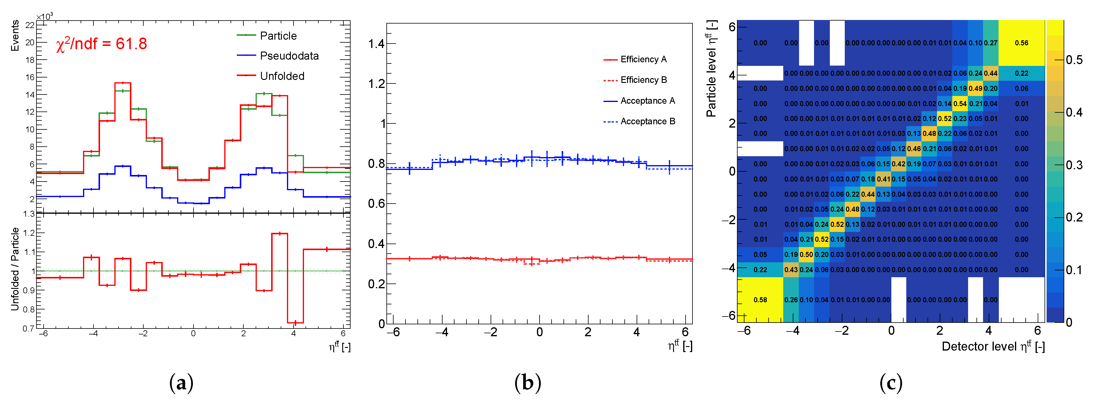
Figure 2.
(a) View of a part of the 16-dimensional log-likelihood function as function of the 6th and 9th bin (b) normalized maximal values of , and (c) normalized maximal values of .
Figure 2.
(a) View of a part of the 16-dimensional log-likelihood function as function of the 6th and 9th bin (b) normalized maximal values of , and (c) normalized maximal values of .

Figure 3.
Marginalized 1D posteriors in the 6th (a) and 9th (b) bin of the spectrum without regularization applied.
Figure 3.
Marginalized 1D posteriors in the 6th (a) and 9th (b) bin of the spectrum without regularization applied.
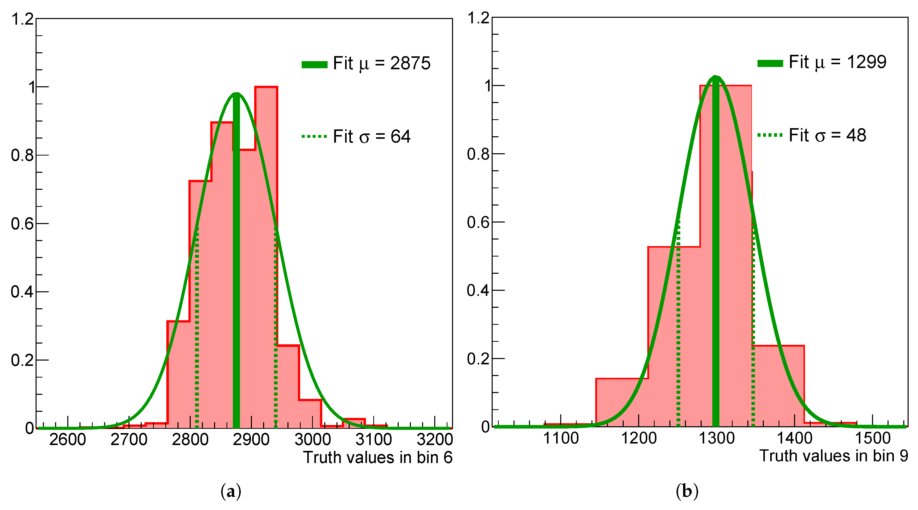
Figure 4.
Unfolding the double-peaked over-binned spectrum for different values of the regularization strength parameter . The parameter is normalized, such that , see Section 3.
Figure 4.
Unfolding the double-peaked over-binned spectrum for different values of the regularization strength parameter . The parameter is normalized, such that , see Section 3.

Figure 5.
Relative as function of the regularization strength parameter and its minimum at . The parameter is normalized, such that , see Section 3. The vertical line represents the minimum of .
Figure 5.
Relative as function of the regularization strength parameter and its minimum at . The parameter is normalized, such that , see Section 3. The vertical line represents the minimum of .

Figure 6.
The envelope of normalized regularization functions in the 6th and 9th bin. For sampling purposes, the gradient of was used.
Figure 6.
The envelope of normalized regularization functions in the 6th and 9th bin. For sampling purposes, the gradient of was used.

Figure 7.
Posterior shifting and narrowing with increasing the regularization strength parameter in a selected single bin: (a) no regularization applied (b) (c) .
Figure 7.
Posterior shifting and narrowing with increasing the regularization strength parameter in a selected single bin: (a) no regularization applied (b) (c) .

Figure 8.
Mostly decreasing (a) curvature, (b) entropy, and (c) derivatives of the unfolded spectrum with respect to . The uncertainty band is evaluated as a standard deviation over 20 independent unfolding runs initiated with different random seeds.
Figure 8.
Mostly decreasing (a) curvature, (b) entropy, and (c) derivatives of the unfolded spectrum with respect to . The uncertainty band is evaluated as a standard deviation over 20 independent unfolding runs initiated with different random seeds.
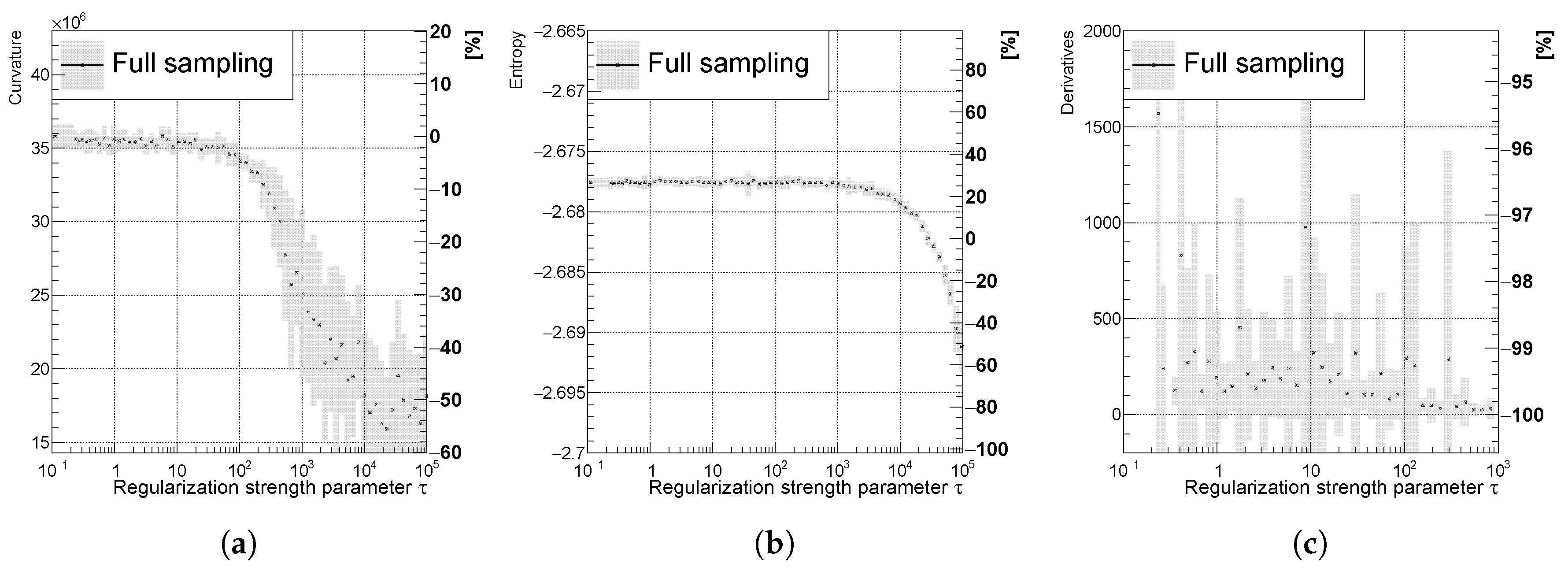
Figure 9.
Cross-bin correlation matrix built from the correlation factor of likelihood, while using the curvature regularization for three different values of .
Figure 9.
Cross-bin correlation matrix built from the correlation factor of likelihood, while using the curvature regularization for three different values of .
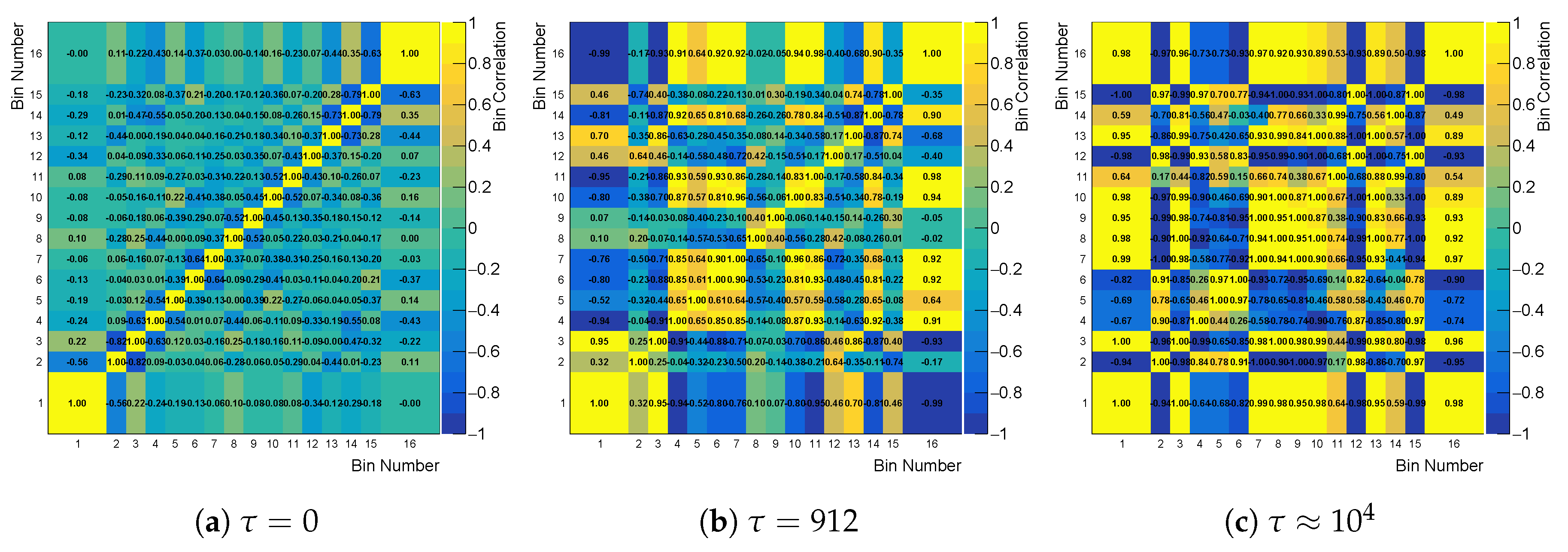
Figure 10.
The averaged cross bin correlations (black) and (pink) using (a) curvature, (b) entropy, and (c) derivative regularization for the spectrum. The uncertainty band is evaluated as a standard deviation over 20 independent unfolding runs initiated with different random seeds.
Figure 10.
The averaged cross bin correlations (black) and (pink) using (a) curvature, (b) entropy, and (c) derivative regularization for the spectrum. The uncertainty band is evaluated as a standard deviation over 20 independent unfolding runs initiated with different random seeds.

Figure 11.
Variable of the spectrum using (a) curvature (b) entropy and (c) derivative regularization illustrating the effect of spectra smoothing. The uncertainty band is evaluated as a standard deviation over 20 independent unfolding runs initiated with different random seeds. The red line indicates the minimal value of the .
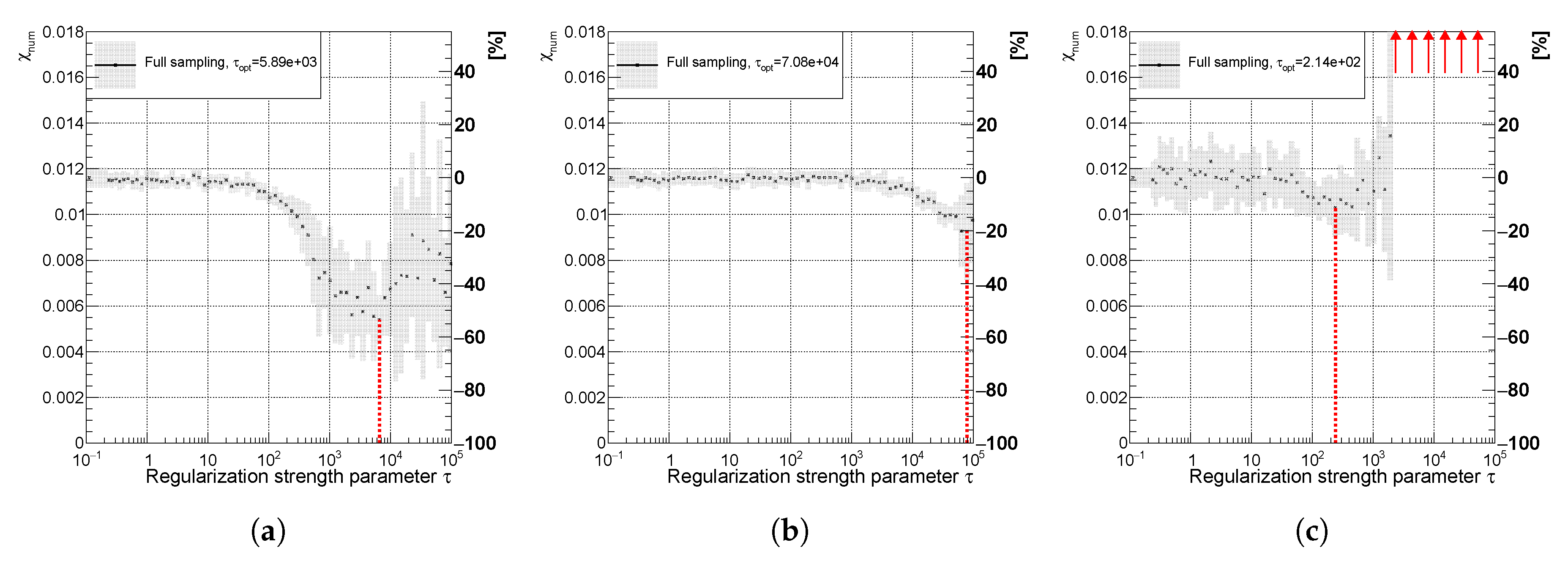
Figure 12.
Variable of the spectrum using (a) curvature, (b) entropy, and (c) derivative regularization illustrating the effect of narrowing the posteriors and decreasing the uncertainty. The uncertainty band is evaluated as a standard deviation over 20 independent unfolding runs initiated with different random seeds.

Figure 13.
Variables and of the spectrum using (a) curvature, (b) entropy, and (c) derivative regularization showing good correspondence. The uncertainty band is evaluated as a standard deviation over 20 independent unfolding runs initiated with different random seeds.
Figure 13.
Variables and of the spectrum using (a) curvature, (b) entropy, and (c) derivative regularization showing good correspondence. The uncertainty band is evaluated as a standard deviation over 20 independent unfolding runs initiated with different random seeds.
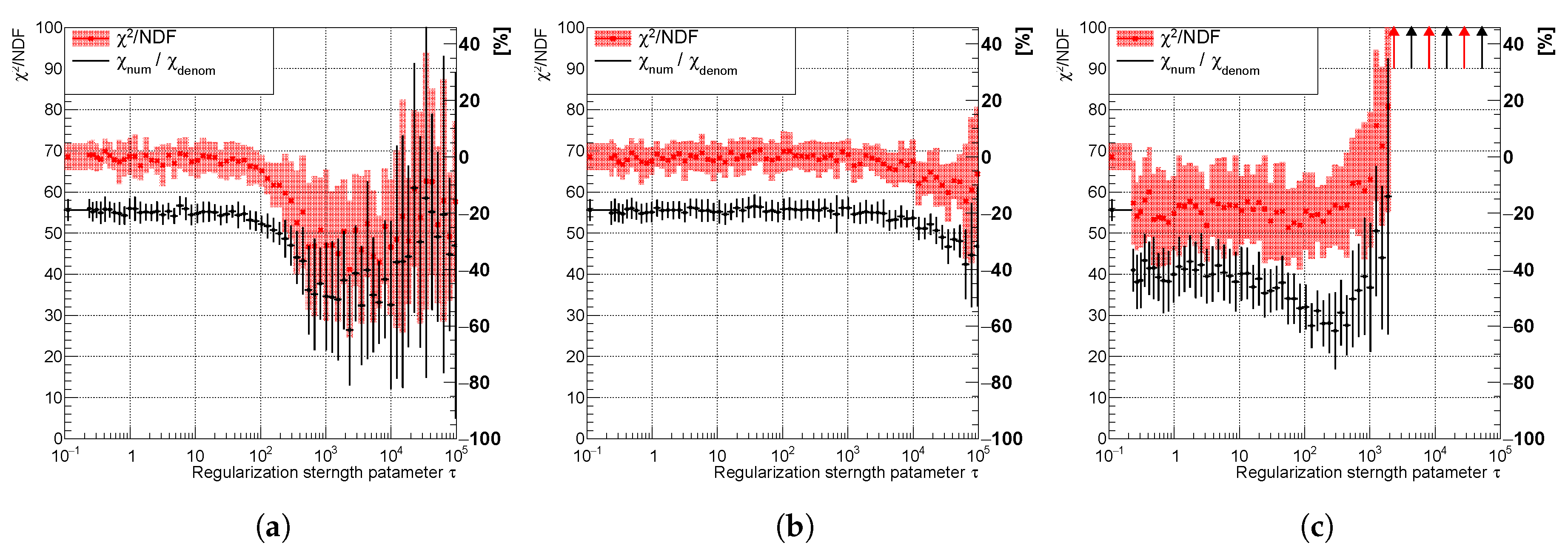
Figure 14.
Variable of the spectrum using (a) curvature, (b) entropy, and (c) derivative regularization comparing combined (faster) sampling (blue) and full sampling (red). The uncertainty band is evaluated as a standard deviation over 20 independent unfolding runs initiated with different random seeds. The vertical dotted lines indicate positions of minima for each sampling case.
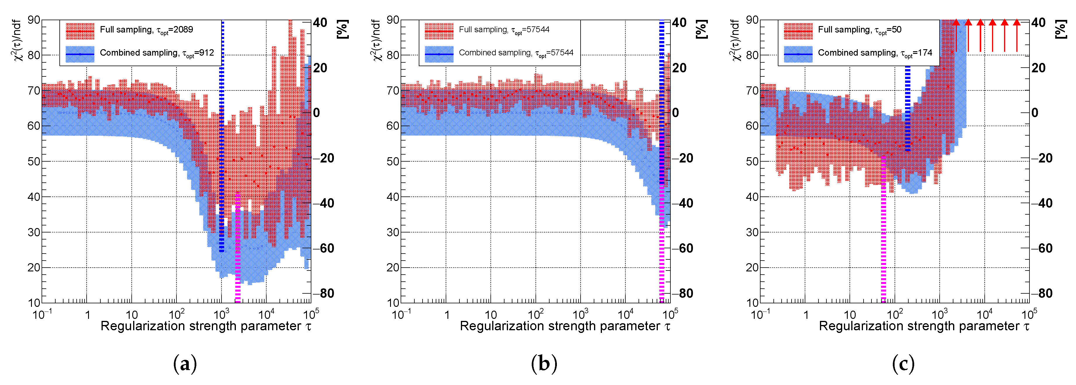
Figure 15.
Variables (a) , (b) for the full sampling method; and (c) using full (red) and combined (blue) sampling of the spectrum with an accidental minimum at (curvature regularization). The vertical dotted lines indicate positions of minima for each sampling case.
Figure 15.
Variables (a) , (b) for the full sampling method; and (c) using full (red) and combined (blue) sampling of the spectrum with an accidental minimum at (curvature regularization). The vertical dotted lines indicate positions of minima for each sampling case.

Figure 16.
The result of unfolding (a) without regularization (b) with regularization and (c) with regularization applied only at second half of the spectrum while using the curvature in the case of a accidental minimum in for one representative random seed.
Figure 16.
The result of unfolding (a) without regularization (b) with regularization and (c) with regularization applied only at second half of the spectrum while using the curvature in the case of a accidental minimum in for one representative random seed.
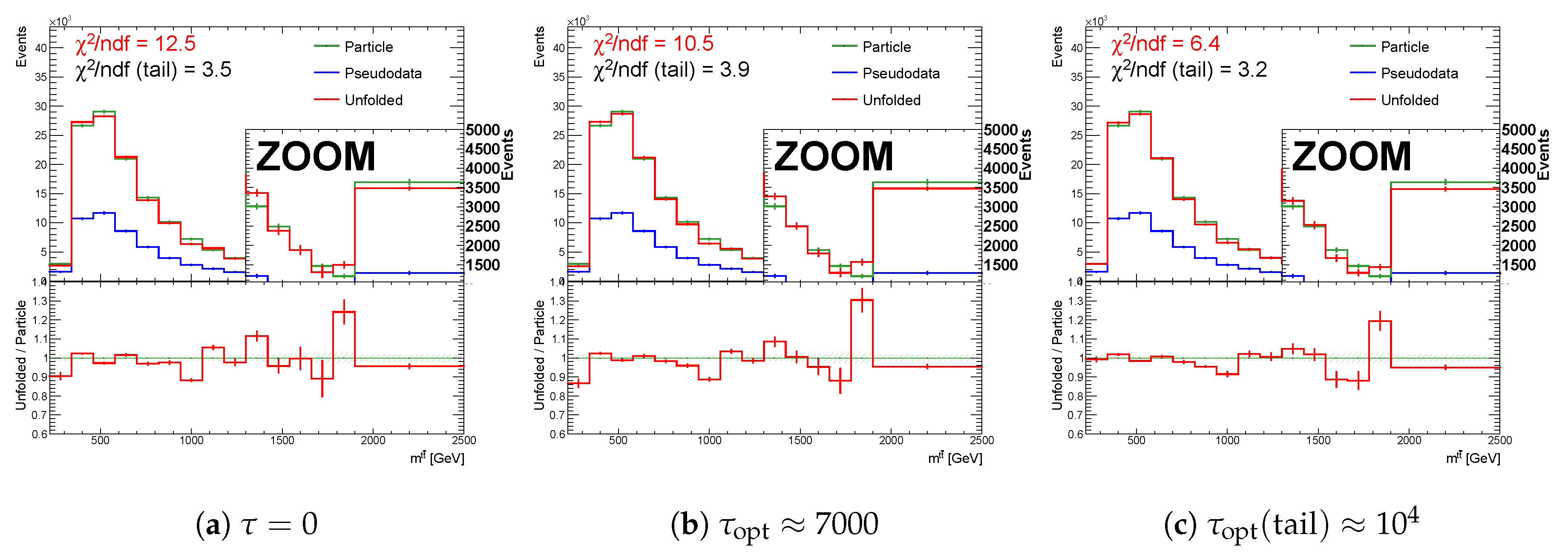
Figure 17.
Variables (a) , (b) for the full sampling method; and, (c) using full (red) and combined (blue) sampling of the spectrum with a vanishing minimum (derivative regularization). The vertical dotted lines indicate positions of minima for each sampling case.
Figure 17.
Variables (a) , (b) for the full sampling method; and, (c) using full (red) and combined (blue) sampling of the spectrum with a vanishing minimum (derivative regularization). The vertical dotted lines indicate positions of minima for each sampling case.

Figure 18.
Result of unfolding (a) without regularization and (b) with regularization of the spectrum using the derivatives in case of a hidden minimum in for one representative random seed. Spectrum becomes smoother, but does not improve due to the narrowing of posteriors.
Figure 18.
Result of unfolding (a) without regularization and (b) with regularization of the spectrum using the derivatives in case of a hidden minimum in for one representative random seed. Spectrum becomes smoother, but does not improve due to the narrowing of posteriors.
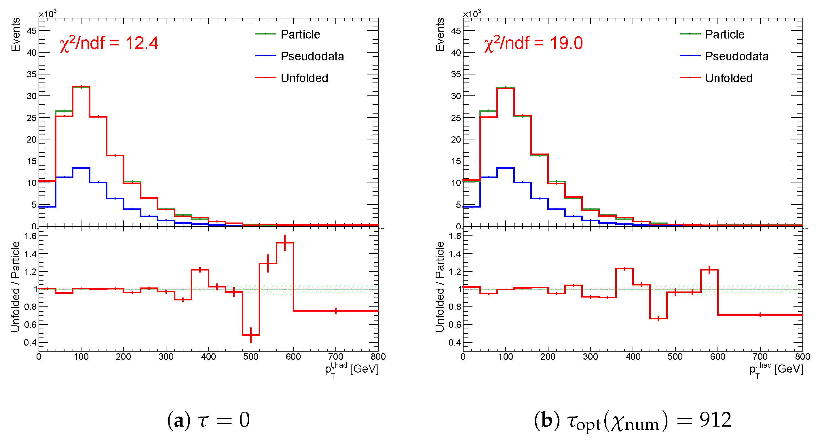
Figure 19.
Variables (a) , (b) for the full sampling method; and (c) using full (red) and combined (blue) sampling of the spectrum with the real minimum at (curvature regularization). The vertical dotted lines indicate positions of minima for each sampling case.
Figure 19.
Variables (a) , (b) for the full sampling method; and (c) using full (red) and combined (blue) sampling of the spectrum with the real minimum at (curvature regularization). The vertical dotted lines indicate positions of minima for each sampling case.

Figure 20.
The result of unfolding (a) without regularization and (b) with regularization of the spectrum while using the curvature in case of a real minimum in for one representative random seed.
Figure 20.
The result of unfolding (a) without regularization and (b) with regularization of the spectrum while using the curvature in case of a real minimum in for one representative random seed.
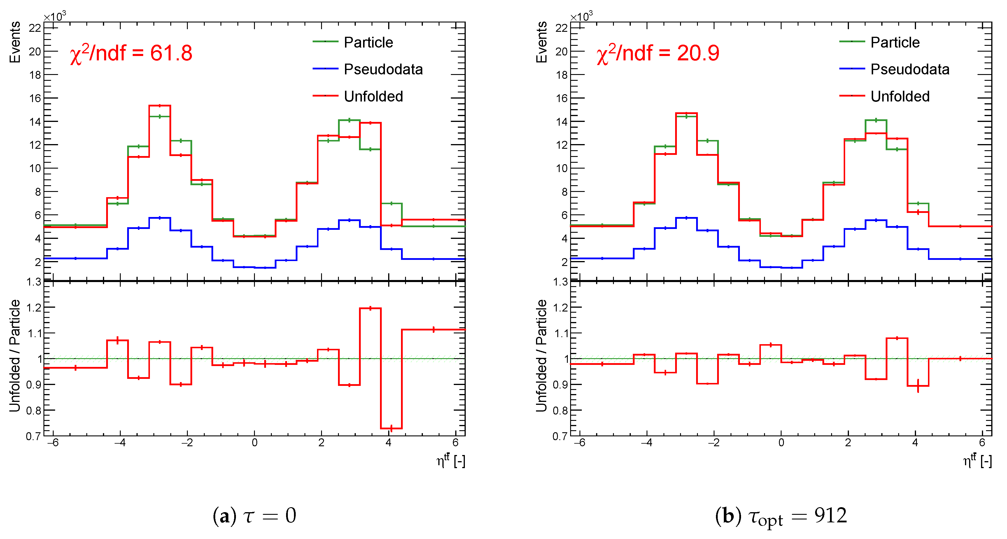
Figure 21.
Result of unfolding (a) without regularization and (c) with regularization of the spectrum using the curvature regularization for one representative random seed. Variable (b) while using full (red) and combined (blue) sampling of the spectrum with minimum at (curvature regularization). In this case, the regularization is not needed. The vertical dotted lines indicate positions of minima for each sampling case.

Figure 22.
Result of unfolding (a) without regularization and (c) with regularization of the spectrum using entropy regularization for one representative random seed. Variable (b) using full (red) and combined (blue) sampling of the spectrum with minimum at (entropy regularization). The vertical dotted lines indicate the positions of minima for each sampling case.

Table 1.
Results of minima type and basic characteristics of the migration matrix M: averaged on-diagonal factor and correlation matrix .
Table 1.
Results of minima type and basic characteristics of the migration matrix M: averaged on-diagonal factor and correlation matrix .
| Spectrum | Type | Minimum | Method | ||
|---|---|---|---|---|---|
| falling | Accidental | Curvature | 0.51 | 0.92 | |
| falling | Hidden | Derivative | 0.48 | 0.86 | |
| double-peaked | Real | Curvature | 0.75 | 0.93 | |
| double-peaked | Real | Curvature | 0.49 | 0.94 | |
| falling | Real | Entropy | 0.29 | 0.86 |
Table 2.
Relative curvature, entropy and derivatives of the unfolded spectra () with respect to the curvature, entropy, and derivatives of the particle level spectra.
Table 2.
Relative curvature, entropy and derivatives of the unfolded spectra () with respect to the curvature, entropy, and derivatives of the particle level spectra.
| Spectrum | Minimum | |||
|---|---|---|---|---|
| Accidental | 1.1 | 1.0 | 2.7 | |
| Hidden | 0.98 | 1.0 | 11 | |
| Real | 1.1 | 1.0 | 0.96 | |
| Real | 3.7 | 1.0 | 3.5 | |
| Real | 14 | 0.97 | 11 |
Table 3.
Time needed to produce curve using combined sampling and full sampling for 68 points of in the region [0; ]. Time in seconds is rounded to hundreds.
Table 3.
Time needed to produce curve using combined sampling and full sampling for 68 points of in the region [0; ]. Time in seconds is rounded to hundreds.
| Spectrum | Minimum | [s] | [s] | |
|---|---|---|---|---|
| Accidental | 900 | 30,700 | 0.029 | |
| Hidden | 1200 | 41,300 | 0.030 | |
| Real | 600 | 14,500 | 0.039 | |
| Real | 1000 | 33,700 | 0.029 | |
| Real | 1300 | 44,700 | 0.030 |
Publisher’s Note: MDPI stays neutral with regard to jurisdictional claims in published maps and institutional affiliations. |
© 2020 by the authors. Licensee MDPI, Basel, Switzerland. This article is an open access article distributed under the terms and conditions of the Creative Commons Attribution (CC BY) license (http://creativecommons.org/licenses/by/4.0/).
Share and Cite
MDPI and ACS Style
Baroň, P.; Kvita, J. Extending the Fully Bayesian Unfolding with Regularization Using a Combined Sampling Method. Symmetry 2020, 12, 2100. https://doi.org/10.3390/sym12122100
AMA Style
Baroň P, Kvita J. Extending the Fully Bayesian Unfolding with Regularization Using a Combined Sampling Method. Symmetry. 2020; 12(12):2100. https://doi.org/10.3390/sym12122100
Chicago/Turabian StyleBaroň, Petr, and Jiří Kvita. 2020. "Extending the Fully Bayesian Unfolding with Regularization Using a Combined Sampling Method" Symmetry 12, no. 12: 2100. https://doi.org/10.3390/sym12122100
Note that from the first issue of 2016, this journal uses article numbers instead of page numbers. See further details here.