Hybrid Cuckoo Search for the Capacitated Vehicle Routing Problem

 ,
,  ,
,
Abstract
1. Introduction
- Adopting a suitable multiple neighborhood structure strategy to improve CS exploration and to help the algorithm to escape from local optima by observe the behaviors of a random sequence of 12 neighborhood structures and then select the most dominant ones to form the best sequence.
- Adopting a suitable selection strategy for exploring the search space to find new solutions and enhance CS exploitation by investigating three selection strategies, namely tournament, rank and disruptive, to find the best-performing one.
- Combining the advantages of CS with those of SA to improve their ability to cooperatively explore the search space and quickly find good solutions within a small region of the search space and also to prevent deterioration.
- Lastly, evaluate the proposed hybrid CS with SA against other state-of-art methods based on average, standard deviation and computational time. The algorithm is furthermore evaluated using Freidman, Holm and Hochberg test, to identify whether there was a significant difference between the proposed algorithm and the best methods in the literature.
2. Related Work
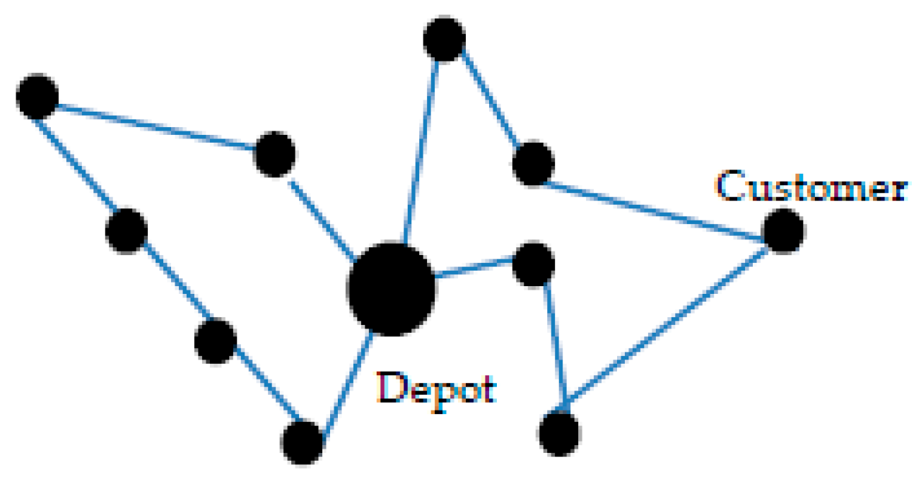
2.1. CVRP Description
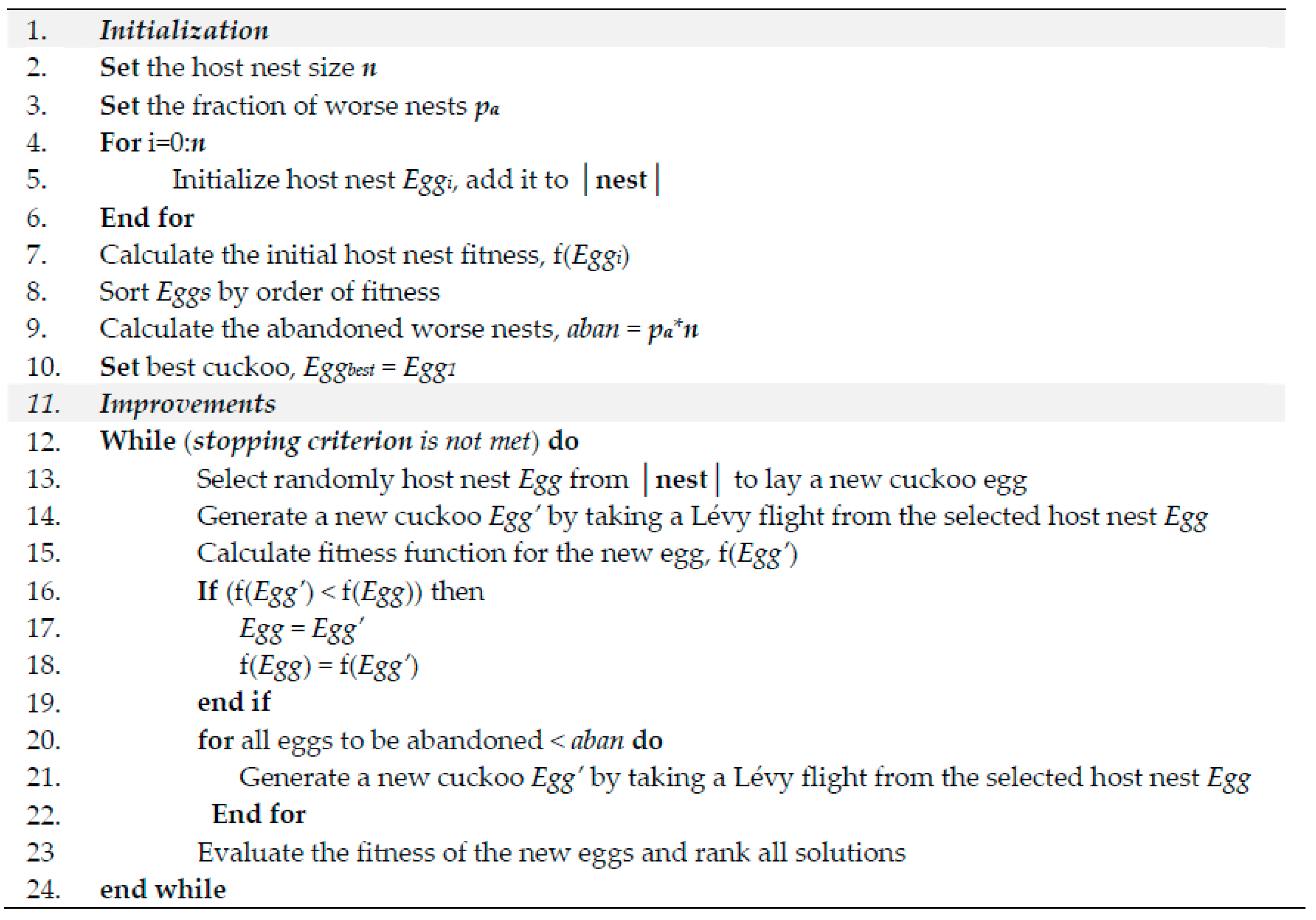
2.2. Standard Cuckoo Search
3. Proposed Method
3.1. Cuckoo Search for CVRP
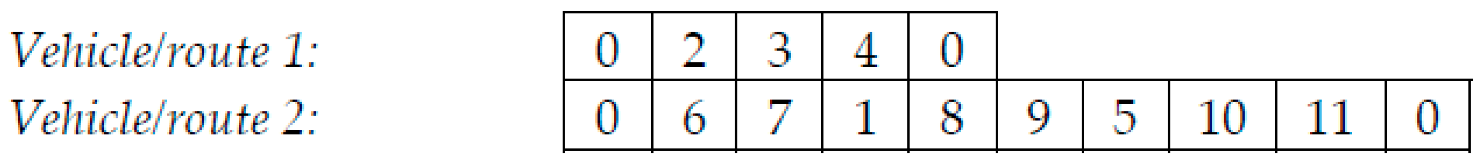
3.1.1. The Egg
3.1.2. The Nest
3.1.3. The Search Space
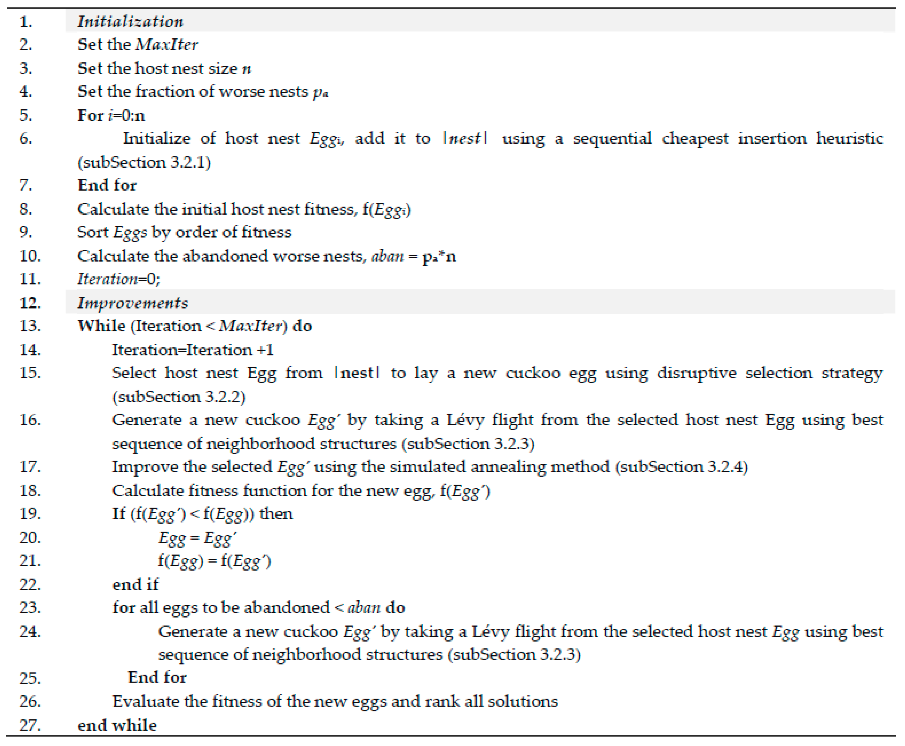
3.2. Propose Discrete Hybrid Cuckoo Search
3.2.1. Initialization of Host Nest Using Sequential Cheapest Insertion Heuristic
3.2.2. Selection of Host Nest Egg to Lay a New Cuckoo Egg
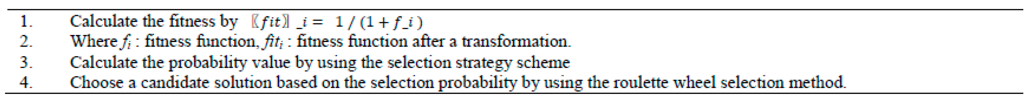
Tournament Selection
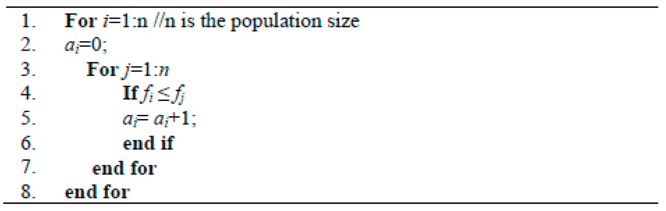
Rank Selection
Disruptive Selection
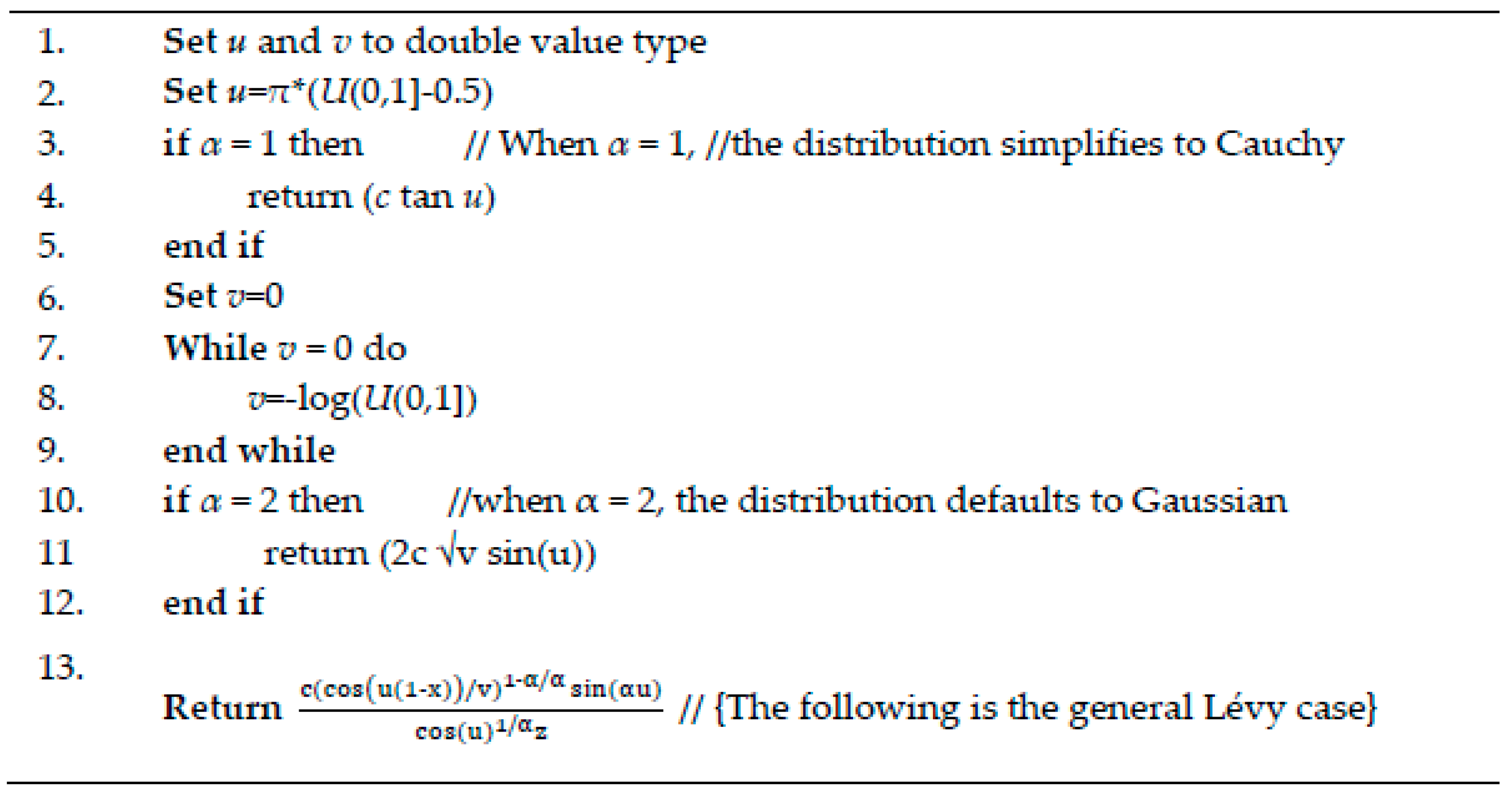
3.2.3. Best Sequence of Neighborhood Structure and Lévy Flight
- [0, i], one step of a small neighborhood structure is performed.
- [(k−1) × i, k × i], one step of a medium neighborhood structure is performed.
- [k × i, 1], a big neighborhood step is performed.
3.2.4. Improve the Egg by Simulated Annealing as a Local Search
4. Experiment Design
- Number of vehicles and customers (column 2 and 3)
- The capacity of each vehicle (column 4)
- Tightness of each problem instance (column 5), which is computed by
- Best-known solution (BKS) of each instance (column 6).
- Experiment 1: First, we investigated the performance of the 12 neighborhood structures to identify the best set of neighborhoods among them and then we formed a sequence based on the knowledge obtained. Second, we investigated which of two acceptance criteria (best, first) was the most suitable for improving the solution. All the neighborhood is evaluated and the best neighborhood is chosen. We were then able to create a neighborhood-enhanced CS (NE-CS) whose performance we compared with that of the basic CS.
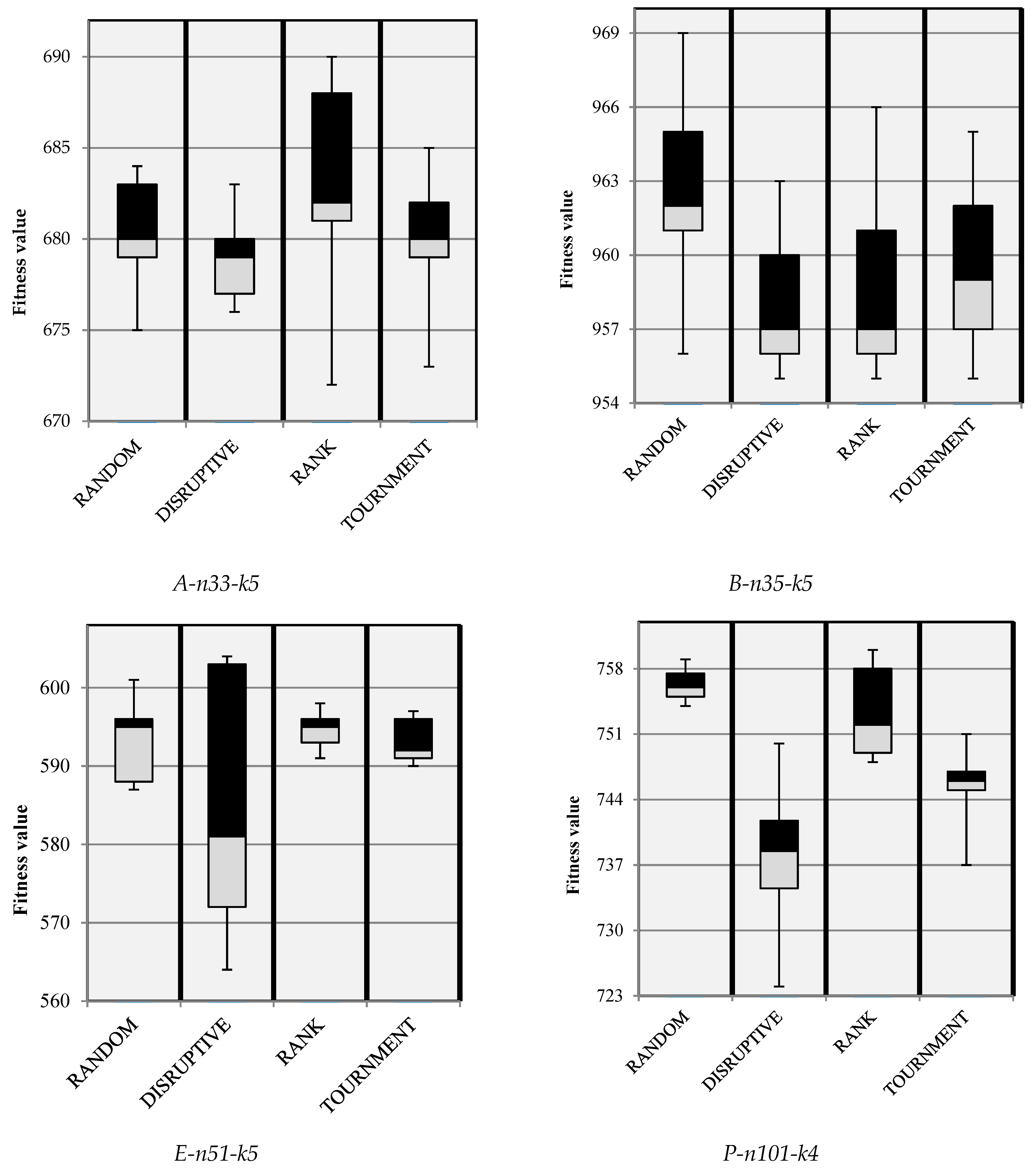
- Experiment 2: We investigated three selection strategies and combined the best-performing one (which we named Discrete Cuckoo Search or Dis-CS) with NE-CS and compared its performance with the output from the first experiment.
- Experiment 3: We hybridized CS with SA (which we named HCS-SA) and compared its performance with the output from the second experiment.
5. Experiment Result
5.1. Results of Comparison of Neighborhood Structures
5.2. Results of Comparison of Accepting Criteria
5.3. Result of Comparison of NE-CS with Basic CS
5.4. Result of Comparison of Selection Strategies
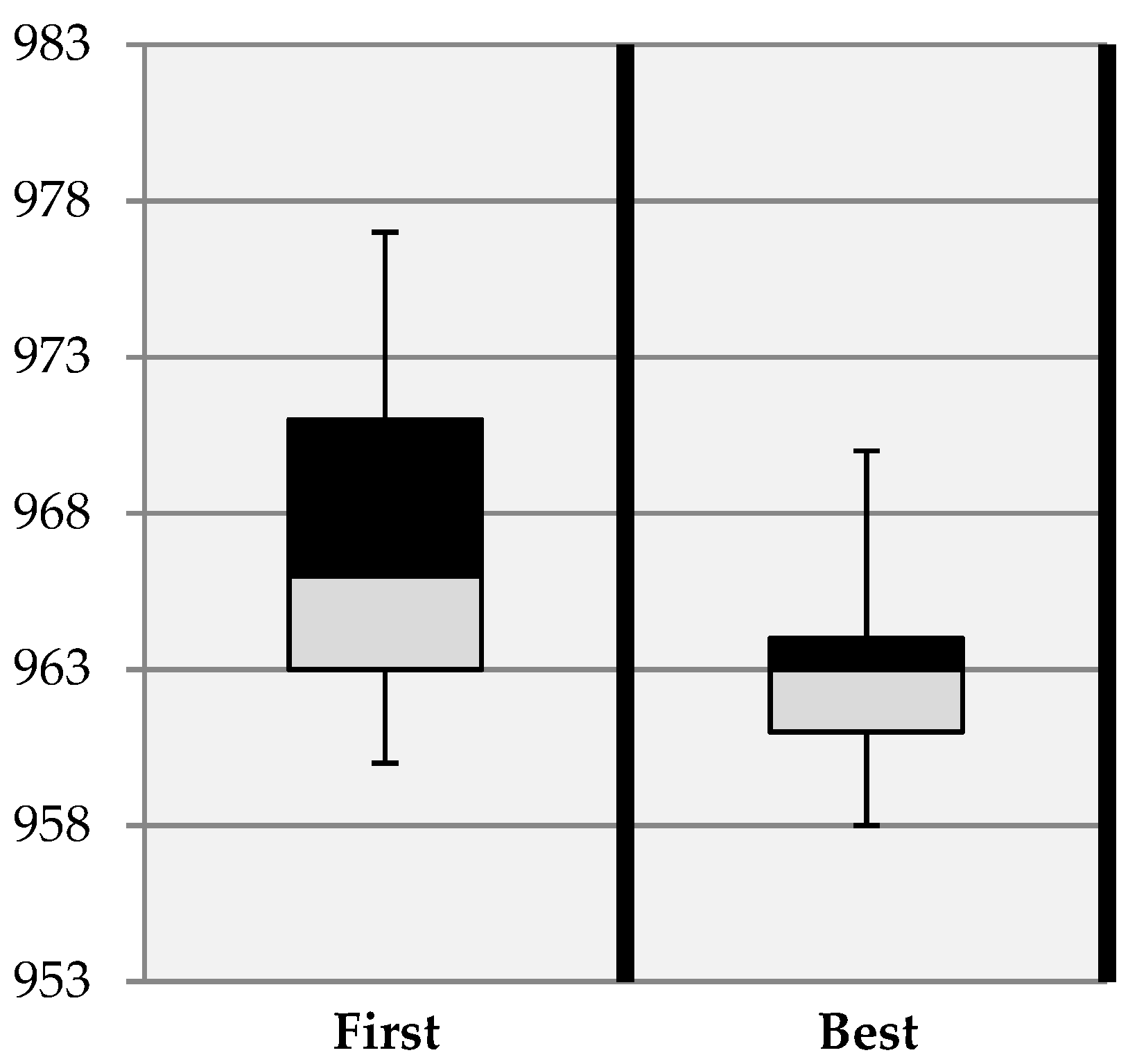
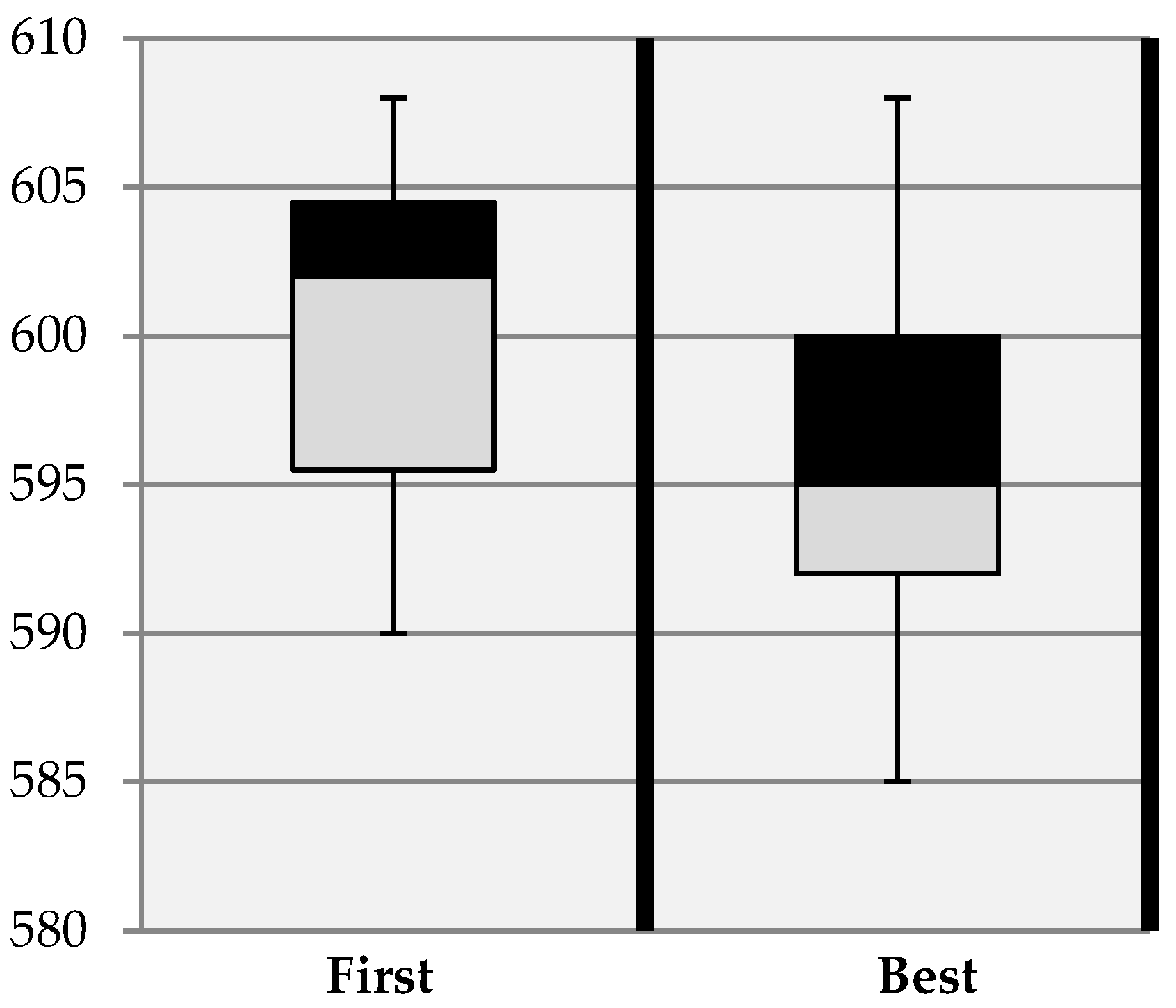
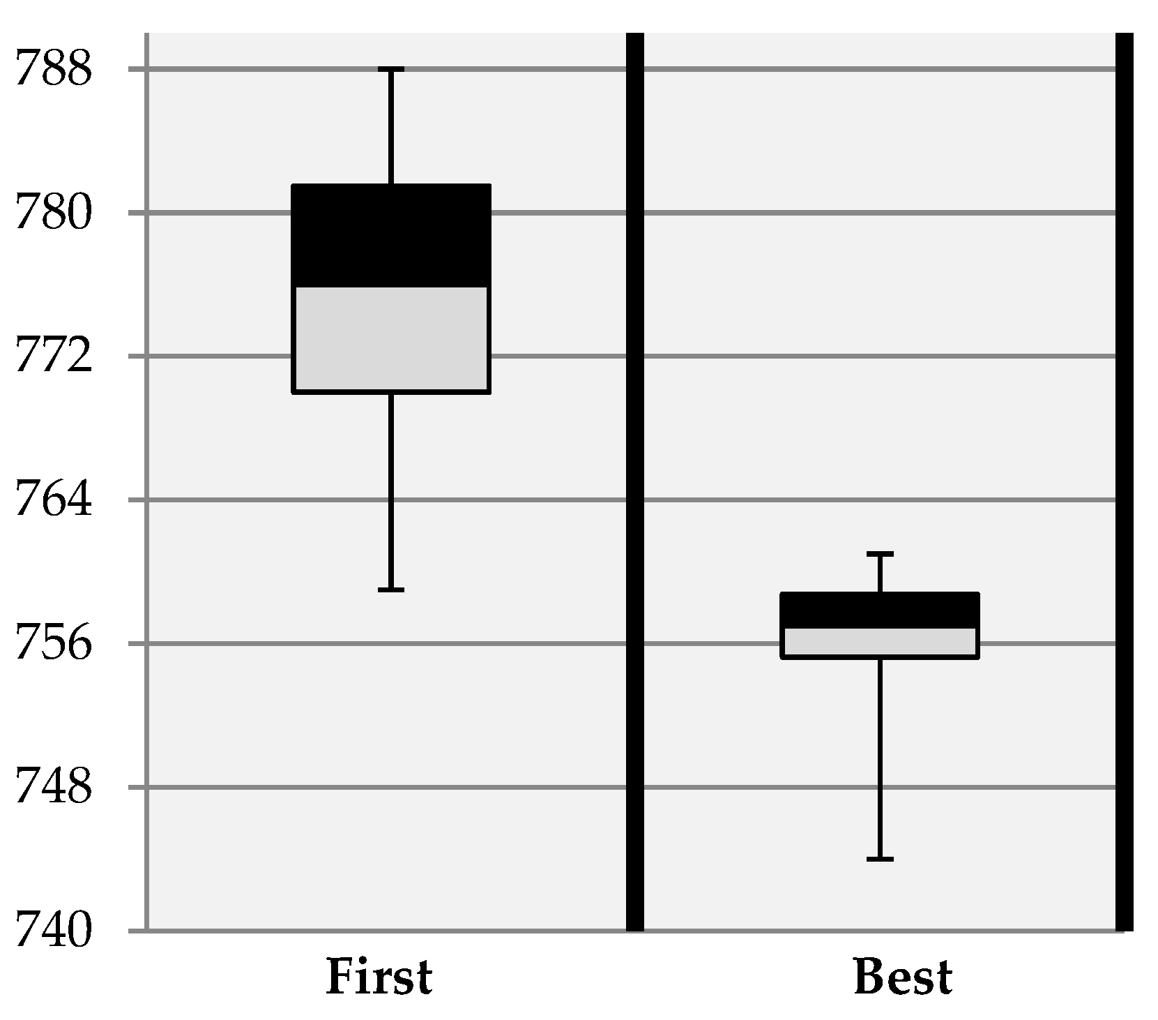
5.5. Result of Comparison of HCS-SA with Dis-CS
5.6. Result of Comparison of HCS-SA with State-of-the-Art Methods
6. Discussion
7. Conclusions
Author Contributions
Funding
Acknowledgments
Conflicts of Interest
References
- Altabeeb, A.M.; Mohsen, A.M.; Ghallab, A. An improved hybrid firefly algorithm for capacitated vehicle routing problem. Appl. Soft Comput. 2019, 84, 105728. [Google Scholar] [CrossRef]
- Alssager, M.; Othman, Z.A. Taguchi-based Parameter Setting of Cuckoo Search Algorithm for Capacitated Vehicle Routing Problem. In Lecture Notes in Electrical Engineering; Springer: Berlin/Heidelberg, Germany, 2016; Volume 387, pp. 71–79. [Google Scholar]
- Kesavan, V.; Kamalakannan, R.; Sudhakarapandian, R.; Sivakumar, P. Heuristic and meta-heuristic algorithms for solving medium and large scale sized cellular manufacturing system NP-hard problems: A comprehensive review. Mater. Today Proc. 2020, 21, 66–72. [Google Scholar] [CrossRef]
- Li, G.; Li, J. An Improved Tabu Search Algorithm for the Stochastic Vehicle Routing Problem with Soft Time Windows. IEEE Access 2020, 8, 158115–158124. [Google Scholar] [CrossRef]
- Yu, V.F.; Redi, A.A.N.P.; Hidayat, Y.A.; Wibowo, O.J. A simulated annealing heuristic for the hybrid vehicle routing problem. Appl. Soft Comput. 2017, 53, 119–132. [Google Scholar] [CrossRef]
- Costa, P.R.D.O.D.; Mauceri, S.; Carroll, P.; Pallonetto, F. A Genetic Algorithm for a Green Vehicle Routing Problem. Electron. Notes Discret. Math. 2018, 64, 65–74. [Google Scholar] [CrossRef]
- Kim, B.-I.; Son, S.-J. A probability matrix based particle swarm optimization for the capacitated vehicle routing problem. J. Intell. Manuf. 2012, 23, 1119–1126. [Google Scholar] [CrossRef]
- Ai, T.J.; Kachitvichyanukul, V. Particle swarm optimization and two solution representations for solving the capacitated vehicle routing problem. Comput. Ind. Eng. 2009, 56, 380–387. [Google Scholar] [CrossRef]
- Chen, A.-L.; Yang, G.-K.; Wu, Z.-M. Hybrid discrete particle swarm optimization algorithm for capacitated vehicle routing problem. J. Zhejiang Univ. A 2006, 7, 607–614. [Google Scholar] [CrossRef]
- Hannan, M.; Akhtar, M.; Begum, R.A.; Basri, H.; Hussain, A.; Scavino, E. Capacitated vehicle-routing problem model for scheduled solid waste collection and route optimization using PSO algorithm. Waste Manag. 2018, 71, 31–41. [Google Scholar] [CrossRef]
- Zainudin, S.; Kerwad, M.M.; Othman, Z.A. A water flow-like algorithm for capacitated vehicle routing problem. J. Theor. Appl. Inf. Technol. 2015, 77, 125–135. [Google Scholar]
- Kerwad, M.M.; Othman, Z.A.; Zainudin, S. Improved water flow-like algorithm for capacitated vehicle routing problem. J. Theor. Appl. Inf. Technol. 2018, 96, 4836–4853. [Google Scholar]
- Niu, Y.; Wang, S.; He, J.; Xiao, J. A novel membrane algorithm for capacitated vehicle routing problem. Soft Comput. 2015, 19, 471–482. [Google Scholar] [CrossRef]
- Faiz, A.; Subiyanto, S.; Arief, U.M. An efficient meta-heuristic algorithm for solving capacitated vehicle routing problem. Int. J. Adv. Intell. Inf. 2018, 4, 212–225. [Google Scholar] [CrossRef]
- Ghodrati, A.; Lotfi, S. A Hybrid CS/PSO Algorithm for Global Optimization. In Proceedings of the Asian Conference on Intelligent Information and Database Systems; Springer: Berlin/Heidelberg, Germany, 2012; Volume 7198, pp. 89–98. [Google Scholar]
- Yang, X.-S.; Deb, S. Cuckoo Search via Lévy flights. In Proceedings of the 2009 World Congress on Nature & Biologically Inspired Computing (NaBIC), Coimbatore, India, 9–11 December 2009; pp. 210–214. [Google Scholar]
- Mohamed, N.S.; Zainudin, S.; Othman, Z.A. Metaheuristic approach for an enhanced mRMR filter method for classification using drug response microarray data. Expert Syst. Appl. 2017, 90, 224–231. [Google Scholar] [CrossRef]
- Usman, A.M.; Yusof, U.K.; Naim, S. Cuckoo inspired algorithms for feature selection in heart disease prediction. Int. J. Adv. Intell. Inf. 2018, 4, 95–106. [Google Scholar] [CrossRef]
- Ouaarab, A.; Ahiod, B.; Yang, X.-S. Improved and Discrete Cuckoo Search for Solving the Travelling Salesman Problem. In Decision Diagrams for Optimization; Springer: Berlin/Heidelberg, Germany, 2013; Volume 516, pp. 63–84. [Google Scholar]
- Iglesias, A.; Gálvez, A.; Suarez, P.; Shinya, M.; Yoshida, N.; Otero, C.; Manchado, C.; Gomez-Jauregui, V. Cuckoo Search Algorithm with Lévy Flights for Global-Support Parametric Surface Approximation in Reverse Engineering. Symmetry 2018, 10, 58. [Google Scholar] [CrossRef]
- Meryem, B.; Abdelmadjid, B. Resolving a vehicle routing problem with heterogeneous fleet, mixed backhauls and time windows using cuckoo behaviour approach. Int. J. Oper. Res. 2015, 24, 132. [Google Scholar] [CrossRef]
- Santillan, J.H.; Tapucar, S.; Manliguez, C.; Calag, V. Cuckoo search via Lévy flights for the capacitated vehicle routing problem. J. Ind. Eng. Int. 2017, 14, 293–304. [Google Scholar] [CrossRef]
- Xiao, L.; Dridi, M.; El Hassani, A.H.; Fei, H.; Lin, W. An Improved Cuckoo Search for a Patient Transportation Problem with Consideration of Reducing Transport Emissions. Sustainability 2018, 10, 793. [Google Scholar] [CrossRef]
- Cordeau, J.-F.; Gendreau, M.; Laporte, G.; Potvin, J.-Y.; Semet, F. A guide to vehicle routing heuristics. J. Oper. Res. Soc. 2002, 53, 512–522. [Google Scholar] [CrossRef]
- Yang, X.S.; Deb, S. Engineering optimisation by cuckoo search. Int. J. Math. Model. Numer. Optim. 2010, 1, 330. [Google Scholar] [CrossRef]
- Xie, J.; Zhou, Y.Q.; Chen, H. A Novel Bat Algorithm Based on Differential Operator and Lévy Flights Trajectory. Comput. Intell. Neurosci. 2013, 2013, 1–13. [Google Scholar] [CrossRef] [PubMed]
- Pavlyukevich, I. Lévy flights, non-local search and simulated annealing. J. Comput. Phys. 2007, 226, 1830–1844. [Google Scholar] [CrossRef]
- Gutowski, M. Lévy flights as an underlying mechanism for global optimization algorithms. arXiv 2001, arXiv:math-ph/0106003. [Google Scholar]
- Wang, G.; Guo, L.; Gandomi, A.H.; Cao, L.; Alavi, A.H.; Duan, H.; Li, J. Lévy-Flight Krill Herd Algorithm. Math. Probl. Eng. 2013, 2013, 1–14. [Google Scholar] [CrossRef]
- Yang, X.-S.; Deb, S. Eagle Strategy Using Lévy Walk and Firefly Algorithms for Stochastic Optimization. In Recent Advances in Computational Optimization; Springer: Berlin/Heidelberg, Germany, 2010; pp. 101–111. [Google Scholar]
- Gandomi, A.H.; Yang, X.-S.; Alavi, A.H. Erratum to: Cuckoo search algorithm: A metaheuristic approach to solve structural optimization problems. Eng. Comput. 2013, 29, 245. [Google Scholar] [CrossRef]
- Akhtar, M.; Hannan, M.; Begum, R.A.; Basri, H.; Scavino, E. Backtracking search algorithm in CVRP models for efficient solid waste collection and route optimization. Waste Manag. 2017, 61, 117–128. [Google Scholar] [CrossRef]
- Bulatović, R.R.; Đorđević, S.R.; Đorđević, V.S. Cuckoo Search algorithm: A metaheuristic approach to solving the problem of optimum synthesis of a six-bar double dwell linkage. Mech. Mach. Theory 2013, 61, 1–13. [Google Scholar] [CrossRef]
- Bhargava, V.; Fateen, S.-E.K.; Bonilla-Petriciolet, A. Cuckoo Search: A new nature-inspired optimization method for phase equilibrium calculations. Fluid Phase Equilibria 2013, 337, 191–200. [Google Scholar] [CrossRef]
- Salomie, I.; Chifu, V.R.; Pop, C.B. Hybridization of Cuckoo Search and Firefly Algorithms for Selecting the Optimal Solution in Semantic Web Service Composition. In Decision Diagrams for Optimization; Springer: Berlin/Heidelberg, Germany, 2013; Volume 516, pp. 217–243. [Google Scholar]
- Laha, D.; Gupta, J.N. An improved cuckoo search algorithm for scheduling jobs on identical parallel machines. Comput. Ind. Eng. 2018, 126, 348–360. [Google Scholar] [CrossRef]
- Yasin, Z.M.; Aziz, N.F.A.; Salim, N.A.; Wahab, N.A.; Rahmat, N.A. Optimal Economic Load Dispatch using Multiobjective Cuckoo Search Algorithm. Indones. J. Electr. Eng. Comput. Sci. 2018, 12, 168. [Google Scholar] [CrossRef]
- Marichelvam, M.K.; Prabaharan, T.; Yang, X. Improved cuckoo search algorithm for hybrid flow shop scheduling problems to minimize makespan. Appl. Soft Comput. 2014, 19, 93–101. [Google Scholar] [CrossRef]
- Ouaarab, A.; Ahiod, B.; Yang, X.-S. Random-key cuckoo search for the travelling salesman problem. Soft Comput. 2015, 19, 1099–1106. [Google Scholar] [CrossRef]
- Lin, J.H.; Lee, I.H. Emotional chaotic cuckoo search for the reconstruction of chaotic dynamics. In Proceedings of the 11th WSEAS International Conference on Mathematical Methods, Computational Techniques and Intelligent Systems and Cybernetics (CIMMACS’12), Singapore, 11–13 May 2012; pp. 123–128. [Google Scholar]
- Walton, S.; Hassan, O.; Morgan, K.; Brown, M. Modified cuckoo search: A new gradient free optimisation algorithm. Chaos Solitons Fractals 2011, 44, 710–718. [Google Scholar] [CrossRef]
- Soneji, H.; Sanghvi, R.C. Towards the improvement of Cuckoo search algorithm. In Proceedings of the 2012 World Congress on Information and Communication Technologies, Trivandrum, India, 30 October–2 November 2012; Institute of Electrical and Electronics Engineers (IEEE): Piscataway, NJ, USA, 2012; pp. 878–883. [Google Scholar]
- Joshi, A.; Kulkarni, O.; Kakandikar, G.; Nandedkar, V. Cuckoo Search Optimization—A Review. Mater. Today Proc. 2017, 4, 7262–7269. [Google Scholar] [CrossRef]
- Shehab, M.; Khader, A.T.; Al-Betar, M.A. A survey on applications and variants of the cuckoo search algorithm. Appl. Soft Comput. 2017, 61, 1041–1059. [Google Scholar] [CrossRef]
- Fister, I.; Yang, X.-S.; Fister, D. Cuckoo Search: A Brief Literature Review. In Recent Advances in Computational Optimization; Springer: Berlin/Heidelberg, Germany, 2013; pp. 49–62. [Google Scholar]
- Yang, X.-S.; Deb, S. Cuckoo search: Recent advances and applications. Neural Comput. Appl. 2014, 24, 169–174. [Google Scholar] [CrossRef]
- Hansen, P.; Mladenović, N. Variable neighborhood search: Principles and applications. Eur. J. Oper. Res. 2001, 130, 449–467. [Google Scholar] [CrossRef]
- Abdullah, S.; Turabieh, H. On the use of multi neighbourhood structures within a Tabu-based memetic approach to university timetabling problems. Inf. Sci. 2012, 191, 146–168. [Google Scholar] [CrossRef]
- Gendreau, M.; Hertz, A.; Laporte, G. New Insertion and Postoptimization Procedures for the Traveling Salesman Problem. Oper. Res. 1992, 40, 1086–1094. [Google Scholar] [CrossRef]
- Hoos, H.H.; Stützle, T. Stochastic Local Search: Foundations & Applications; Stoch. Local Search; Morgan Kaufmann: Burlington, MA, USA, 2005; pp. 61–112. [Google Scholar]
- Goli, A.; Aazami, A.; Jabbarzadeh, A. Accelerated Cuckoo Optimization Algorithm for Capacitated Vehicle Routing Problem in Competitive Conditions. Int. J. Artif. Intell. 2018, 16, 88–112. [Google Scholar]
- Alzaqebah, M.; Abdullah, S. Hybrid Artificial Bee Colony Search Algorithm Based on Disruptive Selection for Examination Timetabling Problems. In Proceedings of the International Conference on Combinatorial Optimization and Applications; Springer: Berlin/Heidelberg, Germany, 2011; pp. 31–45. [Google Scholar]
- Lozano, M.; Cordon, O. Hybrid metaheuristics with evolutionary algorithms specializing in intensification and diversification: Overview and progress report. Comput. Oper. Res. 2010, 37, 481–497. [Google Scholar] [CrossRef]
- Yang, X.-S. Firefly Algorithm, Lévy Flights and Global Optimization. In Research and Development in Intelligent Systems XXVI; Springer: Berlin/Heidelberg, Germany, 2010; pp. 209–218. [Google Scholar]
- Teymourian, E.; Kayvanfar, V.; Komaki, G.; Zandieh, M. Enhanced intelligent water drops and cuckoo search algorithms for solving the capacitated vehicle routing problem. Inf. Sci. 2016, 334, 354–378. [Google Scholar] [CrossRef]
- Jaddi, N.S.; Abdullah, S.; Malek, M.A. Master-Leader-Slave Cuckoo Search with Parameter Control for ANN Optimization and Its Real-World Application to Water Quality Prediction. PLoS ONE 2017, 12, e0170372. [Google Scholar] [CrossRef]
- Ilunga-Mbuyamba, E.; Cruz-Duarte, J.M.; Avina-Cervantes, J.G.; Correa-Cely, C.R.; Lindner, D.; Chalopin, C. Active contours driven by Cuckoo Search strategy for brain tumour images segmentation. Expert Syst. Appl. 2016, 56, 59–68. [Google Scholar] [CrossRef]
- Viswanathan, G.M.; Afanasyev, V.; Buldyrev, S.V.; Murphy, E.J.; Prince, P.A.; Stanley, H. Lévy flight search patterns of wandering albatrosses. Nat. Cell Biol. 1996, 381, 413–415. [Google Scholar] [CrossRef]
- Amirsadri, S.; Mousavirad, S.J.; Ebrahimpour-Komleh, H. A Levy flight-based grey wolf optimizer combined with back-propagation algorithm for neural network training. Neural Comput. Appl. 2017, 30, 3707–3720. [Google Scholar] [CrossRef]
- Hakli, H.; Uğuz, H. A novel particle swarm optimization algorithm with Levy flight. Appl. Soft Comput. 2014, 23, 333–345. [Google Scholar] [CrossRef]
- Sharma, H.; Bansal, J.C.; Arya, K.V.; Yang, X.-S. Lévy flight artificial bee colony algorithm. Int. J. Syst. Sci. 2016, 47, 2652–2670. [Google Scholar] [CrossRef]
- Alssager, M.; Othman, Z.A. Cuckoo search algorithm for capacitated vehicle routing problem. J. Theor. Appl. Inf. Technol. 2016, 88, 11–19. [Google Scholar]
- Sterling, K.B. Cuckoo: Cheating by nature. Choice Rev. Online 2015, 53, 53. [Google Scholar] [CrossRef]
- Blickle, T.; Thiele, L. A mathematical analysis of tournament selection. In Proceedings of the 6th International Conference on Genetic Algorithms; Morgan Kaufmann Publishers Inc.: San Francisco, CA, USA, 1995; pp. 9–16. ISBN 1558603700. [Google Scholar]
- Bao, L.; Zeng, J.-C. Comparison and Analysis of the Selection Mechanism in the Artificial Bee Colony Algorithm. In Proceedings of the 2009 Ninth International Conference on Hybrid Intelligent Systems, Shenyang, China, 12–14 August 2009; Institute of Electrical and Electronics Engineers (IEEE): Piscataway, NJ, USA, 2009; Volume 1, pp. 411–416. [Google Scholar]
- Song, A.; Lu, J. Ranking based adaptive evolutionary operator genetic algorithm. Tien Tzu Hsueh Pao 1999, 27, 85–88. [Google Scholar]
- Osman, I.H. Metastrategy simulated annealing and tabu search algorithms for the vehicle routing problem. Ann. Oper. Res. 1993, 41, 421–451. [Google Scholar] [CrossRef]
- Husselmann, A.V.; Hawick, K.A. Levy flights for particle swarm optimisation algorithms on graphical processing units. Parallel Cloud Comput. 2013, 2, 32–40. [Google Scholar]
- Ouaarab, A.; Ahiod, B.; Yang, X.-S. Discrete cuckoo search algorithm for the travelling salesman problem. Neural Comput. Appl. 2014, 24, 1659–1669. [Google Scholar] [CrossRef]
- Burke, E.K.; Kendall, G. Search Methodologies; Springer: Berlin/Heidelberg, Germany, 2005. [Google Scholar]
- Kao, Y.; Chen, M.-H.; Huang, Y.-T. A Hybrid Algorithm Based on ACO and PSO for Capacitated Vehicle Routing Problems. Math. Probl. Eng. 2012, 2012, 1–17. [Google Scholar] [CrossRef]
- Cui, L.; Wang, L.; Deng, J.; Zhang, J. A New Improved Quantum Evolution Algorithm with Local Search Procedure for Capacitated Vehicle Routing Problem. Math. Probl. Eng. 2013, 2013, 1–17. [Google Scholar] [CrossRef]
- Ammi, M.; Chikhi, S. An island model based genetic algorithm for solving the capacitated vehicle routing problem. In Proceedings of the 6th International Conference of Soft Computing and Pattern Recognition (SoCPaR), Tunis, Tunisia, 11–14 August 2014; Institute of Electrical and Electronics Engineers (IEEE): Piscataway, NJ, USA, 2014; pp. 342–347. [Google Scholar]
- Ruttanateerawichien, K.; Kurutach, W.; Pichpibul, T. An Improved Golden Ball Algorithm for the Capacitated Vehicle Routing Problem. In Cyberspace Data and Intelligence, and Cyber-Living, Syndrome, and Health; Springer Science and Business Media LLC: Berlin/Heidelberg, Germany, 2014; Volume 472, pp. 341–356. [Google Scholar]
- Wedyan, A.; Narayanan, A. Solving capacitated vehicle routing problem using intelligent water drops algorithm. In Proceedings of the 10th International Conference on Natural Computation (ICNC), Xiamen, China, 19–21 August 2014; Institute of Electrical and Electronics Engineers (IEEE): Piscataway, NJ, USA, 2014; pp. 469–474. [Google Scholar]
- Rizkallah, L.W.; Ahmed, M.F.; Darwish, N.M. SMT-LH: A New Satisfiability Modulo Theory-Based Technique for Solving Vehicle Routing Problem with Time Window Constraints. Comput. J. 2019. [Google Scholar] [CrossRef]
- Wang, J.; Ren, W.; Zhang, Z.; Huang, H.; Zhou, Y. A Hybrid Multiobjective Memetic Algorithm for Multiobjective Periodic Vehicle Routing Problem with Time Windows. IEEE Trans. Syst. Man Cybern. Syst. 2020, 50, 4732–4745. [Google Scholar] [CrossRef]
- Khoo, T.-S.; Mohammad, B.B.; Wong, V.-H.; Tay, Y.-H.; Nair, M.B. A Two-Phase Distributed Ruin-and-Recreate Genetic Algorithm for Solving the Vehicle Routing Problem with Time Windows. IEEE Access 2020, 8, 169851–169871. [Google Scholar] [CrossRef]
- Zhao, L.; Cao, N. Fuzzy Random Chance-Constrained Programming Model for the Vehicle Routing Problem of Hazardous Materials Transportation. Symmetry 2020, 12, 1208. [Google Scholar] [CrossRef]
- Kucharska, E. Dynamic Vehicle Routing Problem—Predictive and Unexpected Customer Availability. Symmetry 2019, 11, 546. [Google Scholar] [CrossRef]
- Wang, X.; Shao, S.; Tang, J. Iterative Local-Search Heuristic for Weighted Vehicle Routing Problem. IEEE Trans. Intell. Transp. Syst. 2020, 1–11. [Google Scholar] [CrossRef]
- Mehlawat, M.K.; Gupta, P.; Khaitan, A.; Pedrycz, W. A Hybrid Intelligent Approach to Integrated Fuzzy Multiple Depot Capacitated Green Vehicle Routing Problem with Split Delivery and Vehicle Selection. IEEE Trans. Fuzzy Syst. 2020, 28, 1155–1166. [Google Scholar] [CrossRef]
- Zhang, Z.; Qin, H.; Li, Y. Multi-Objective Optimization for the Vehicle Routing Problem with Outsourcing and Profit Balancing. IEEE Trans. Intell. Transp. Syst. 2020, 21, 1987–2001. [Google Scholar] [CrossRef]


| Natural Cuckoo Bird Behavior | Cuckoo Search Algorithm |
|---|---|
| Host nest | Solution container (new/old solution) |
| Host nest egg | Old solution |
| Cuckoo bird egg | New solution |
| Abandoned nest/egg | Worst solution |
| Name | Category | Details |
|---|---|---|
| SHIFT-1-0 | Inter-route | One customer is transferred from one route to another route. |
| SWAP-1-1 | Inter-route | Swap one customer from one route with one customer from another route. |
| SHIFT-2-0 | Inter-route | Move two adjacent customers from one route to another route. |
| SWAP-2-1 | Inter-route | Swap two adjacent customers from one route with one customer from another route. |
| SWAP-2-2 | Inter-route | Swap two adjacent customers from one route with two adjacent customers from another route. |
| CROSS | Inter-route | The arc between two adjacent customers i and j belonging to a route one and the arc between two adjacent customers i′ and j′ belonging to route two are both removed. Next an arc is inserted connecting i and j′ and another is inserted linking i′ and j. |
| K-SHIFT | Inter-route | A subset of consecutive customers is transferred from a route one to the end of a route two. |
| REINSERTION | Intra-route | One customer is removed and later inserted into other position of the route. |
| OR-OPT2 | Intra-route | Two adjacent customers are removed and later inserted into other position of the route. |
| OR-OPT3 | Intra-route | Three adjacent customers are removed and later inserted into other position of the route. |
| TWO-OPT | Intra-route | Two nonadjacent arcs are deleted and later other two are added in such a way that a new route is generated. |
| EXCHANGE | Intra-route | Permutation of two customers being swapped. |
| Step Length Generated by Lévy Flight | Neighborhood Structures Used | |
|---|---|---|
| 1 | {0, i} = (0, 0.07) | SHIFT-1-0 |
| 2 | {i, i × 2} = (0.07, 0.14) | SWAP-1-1 |
| 3 | {i × 2, i × 3} = (0.14, 0.21) | SHIFT-2-0 |
| 4 | {i × 3, i × 4} = (0.21, 0.28) | REINSERTION |
| 5 | {i × 4, i × 5} = (0.28, 0.35) | OR-OPT2 |
| 6 | {i × 5, i × 6} = (0.35, 0.42) | OR-OPT3 |
| 7 | {i × 6, i × 7} = (0.42, 0.49) | TWO-OPT |
| 8 | {i × 7, i × 8} = (0.49, 0.56) | EXCHANGE |
| 9 | {i × 8, i × 9} = (0.56, 0.63) | SWAP-2-1 |
| 10 | {i × 9, i × 10} = (0.63, 0.7) | SWAP-2-2 |
| 11 | {i × 10, i × 11} = (0.7, 0.77) | CROSS |
| 12 | {i × 11, 1} = (0.77, 1) | K-SHIFT |
| Instance | V | Cs | Ca | Ti | BKS |
|---|---|---|---|---|---|
| A-n33-k5 | 5 | 32 | 100 | 0.82 | 661 |
| A-n46-k7 | 7 | 45 | 100 | 0.86 | 914 |
| A-n60-k9 | 9 | 59 | 100 | 0.92 | 1354 |
| B-n35-k5 | 5 | 34 | 100 | 0.87 | 955 |
| B-n45-k5 | 5 | 44 | 100 | 0.97 | 751 |
| B-n68-k9 | 9 | 67 | 100 | 0.93 | 1272 |
| B-n78-k10 | 10 | 77 | 100 | 0.94 | 1221 |
| E-n30-k3 | 3 | 29 | 4500 | 0.94 | 534 |
| E-n51-k5 | 5 | 50 | 160 | 0.97 | 521 |
| E-n76-k7 | 7 | 75 | 220 | 0.89 | 682 |
| F-n72-k4 | 4 | 71 | 30,000 | 0.96 | 237 |
| F-n135-k7 | 7 | 134 | 2210 | 0.95 | 1162 |
| M-n101-k10 | 10 | 100 | 200 | 0.91 | 820 |
| M-n121-k7 | 7 | 120 | 200 | 0.98 | 1034 |
| P-n76-k4 | 4 | 75 | 350 | 0.97 | 593 |
| P-n101-k4 | 4 | 100 | 400 | 0.91 | 681 |
| Parameter | Value |
|---|---|
| Initial temperature | 100 set in the preliminary experiment as in Table 6 |
| Final temperature | 0.5 as suggested by Reference [70] |
| Cooling schedule | 0.99 as suggested by Reference [70] |
| Instance | Initial Temperatures | ||
|---|---|---|---|
| 50 | 100 | 200 | |
| A-n33-k5 | 671 | 661 | 669 |
| B-n35-k5 | 966 | 965 | 960 |
| E-n51-k5 | 559 | 542 | 568 |
| P-n101-k4 | 715 | 720 | 716 |
| Neigh | ANF | AAI | SPR | RK | |
|---|---|---|---|---|---|
| 1. | SHIFT-1-0 | 16.8 | 15.9 | 94.8 | 5 |
| 2. | SHIFT-2-0 | 16.1 | 9.4 | 58.5 | 11 |
| 3. | SWAP-1-1 | 16.2 | 13.2 | 81.2 | 7 |
| 4. | SWAP-1-2 | 17.5 | 13.7 | 78.3 | 8 |
| 5. | SWAP-2-2 | 16.1 | 10.1 | 62.3 | 10 |
| 6. | CROSS | 16.9 | 12.0 | 70.8 | 9 |
| 7. | K-SHIFT | 16.1 | 7.1 | 43.9 | 12 |
| 8. | REINSERTION | 16.4 | 16.4 | 99.9 | 1 |
| 9. | OR-OPT2 | 16.9 | 16.5 | 97.3 | 4 |
| 10. | OR-OPT3 | 16.6 | 15.8 | 94.7 | 6 |
| 11. | TWO-OPT | 16.1 | 16.1 | 99.5 | 2 |
| 12. | EXCHANGE | 17.1 | 17.0 | 99 | 3 |
| Average | 16.6 | 13.6 | |||
| Total frequency | 199 | 163 | |||
| Instance | BKS | CS | NE-CS | Computational Time (s) | |||||||
|---|---|---|---|---|---|---|---|---|---|---|---|
| Min. | Avg. | Std. | Max. | Min. | Avg. | Std. | Max. | CS | NE-CS | ||
| A-n33-k5 | 661 | 688 | 692.0 | 16.67 | 723 | 678 | 684.8 | 4.56 | 694 | 11.49 | 3.391 |
| A-n46-k7 | 914 | 973 | 994.76 | 8.05 | 1011 | 966 | 975.45 | 6.05 | 985 | 12.15 | 8.782 |
| A-n60-k9 | 1354 | 1414 | 1413.49 | 11.16 | 1436 | 1401 | 1412.6 | 9.24 | 1431 | 17.89 | 12.72 |
| B-n35-k5 | 955 | 962 | 966.37 | 24.87 | 973 | 955 | 961.54 | 4.84 | 970 | 22.42 | 5.31 |
| B-n45-k5 | 751 | 770 | 794.88 | 10.45 | 793 | 769 | 785.90 | 8.16 | 796 | 12.91 | 5.62 |
| B-n68-k9 | 1272 | 1320 | 1326.73 | 15.39 | 1333 | 1303 | 1310.6 | 4.31 | 1317 | 39.94 | 24.44 |
| B-n78-k10 | 1221 | 1284 | 1307.94 | 26.79 | 1323 | 1281 | 1301.6 | 13.00 | 1322 | 38.86 | 27.18 |
| E-n30-k3 | 534 | 565 | 559.07 | 24.41 | 568 | 545 | 555.18 | 4.40 | 560 | 20.19 | 6.67 |
| E-n51-k5 | 521 | 590 | 618.28 | 7.98 | 613 | 586 | 599.54 | 6.94 | 609 | 31.33 | 14.38 |
| E-n76-k7 | 682 | 746 | 763.69 | 22.25 | 786 | 742 | 755.54 | 9.24 | 768 | 59.25 | 56.62 |
| F-n72-k4 | 237 | 255 | 265.27 | 19.35 | 278 | 245 | 249.18 | 3.84 | 258 | 81.12 | 80.41 |
| F-n135-k7 | 1162 | 1301 | 1319.58 | 11.32 | 1327 | 1289 | 1310.9 | 10.83 | 1329 | 1178.8 | 1165.8 |
| M-n101-k10 | 820 | 844 | 843.69 | 12.84 | 870 | 836 | 841.36 | 3.32 | 846 | 41.46 | 24.51 |
| M-n121-k7 | 1034 | 1088 | 1110.22 | 15.11 | 1107 | 1086 | 1094.8 | 6.58 | 1106 | 140.85 | 126.45 |
| P-n76-k4 | 593 | 679 | 688.27 | 8.72 | 694 | 676 | 686.63 | 5.95 | 693 | 67.78 | 66.65 |
| P-n101-k4 | 681 | 758 | 760.75 | 14.16 | 766 | 744 | 753.45 | 5.16 | 761 | 175.46 | 167.47 |
| Instance | p-Value |
|---|---|
| A-n33-k5 | 0.000 |
| A-n46-k7 | 0.000 |
| A-n60-k9 | 0.008 |
| B-n35-k5 | 0.001 |
| B-n45-k5 | 0.000 |
| B-n68-k9 | 0.000 |
| B-n78-k10 | 0.000 |
| E-n30-k3 | 0.029 |
| E-n51-k5 | 0.000 |
| E-n76-k7 | 0.000 |
| F-n72-k4 | 0.000 |
| F-n135-k7 | 0.001 |
| M-n101-k10 | 0.000 |
| M-n121-k7 | 0.000 |
| P-n76-k4 | 0.02 |
| P-n101-k4 | 0.11 |
| Instance | BKS | NE-CS | Tour-CS | Rank-CS | Dis-CS | ||||||||||||
|---|---|---|---|---|---|---|---|---|---|---|---|---|---|---|---|---|---|
| Min. | Avg. | Std. | Max. | Min. | Avg. | Std. | Max. | Min. | Avg. | Std. | Max. | Min. | Avg. | Std. | Max. | ||
| A-n33-k5 | 661 | 678 | 684.8 | 4.56 | 694 | 662 | 683.7 | 5.0 | 691 | 661 | 686.2 | 3.7 | 691 | 661 | 685.1 | 3.5 | 689 |
| A-n46-k7 | 914 | 966 | 975.45 | 6.05 | 985 | 966 | 977.8 | 5.7 | 990 | 956 | 977.8 | 7.4 | 991 | 914 | 979.9 | 8.9 | 982 |
| A-n60-k9 | 1354 | 1401 | 1412.6 | 9.24 | 1431 | 1374 | 1415.2 | 11.0 | 1425 | 1404 | 1420.6 | 8.6 | 1439 | 1369 | 1400.6 | 13.4 | 1419 |
| B-n35-k5 | 955 | 955 | 961.54 | 4.84 | 970 | 955 | 963.6 | 4.4 | 872 | 955 | 964.1 | 6.3 | 975 | 955 | 960.4 | 4.7 | 972 |
| B-n45-k5 | 751 | 769 | 785.90 | 8.16 | 796 | 768 | 789.0 | 8.0 | 799 | 751 | 790.0 | 7.1 | 802 | 759 | 774.9 | 10.0 | 793 |
| B-n68-k9 | 1272 | 1303 | 1310.6 | 4.31 | 1317 | 1299 | 1311.8 | 5.8 | 1323 | 1301 | 1313.5 | 5.3 | 1322 | 1290 | 1303.3 | 4.6 | 1311 |
| B-n78-k10 | 1221 | 1281 | 1301.6 | 13.0 | 1322 | 1286 | 1306.6 | 9.3 | 1322 | 1282 | 1314.2 | 7.4 | 1325 | 1261 | 1287 | 14.4 | 1310 |
| E-n30-k3 | 534 | 545 | 555.18 | 4.40 | 560 | 534 | 556.7 | 3.6 | 563 | 546 | 556.9 | 3.7 | 566 | 534 | 554.9 | 4.2 | 559 |
| E-n51-k5 | 521 | 586 | 599.54 | 6.94 | 609 | 586 | 598.2 | 5.2 | 607 | 590 | 599.9 | 5.5 | 611 | 562 | 585.2 | 12.9 | 605 |
| E-n76-k7 | 682 | 742 | 755.54 | 9.24 | 768 | 752 | 760.3 | 5.5 | 771 | 758 | 754.9 | 3.5 | 774 | 732 | 751.6 | 9.9 | 766 |
| F-n72-k4 | 237 | 245 | 249.18 | 3.84 | 258 | 247 | 253.1 | 3.0 | 259 | 247 | 255.3 | 3.6 | 262 | 237 | 245.4 | 3.6 | 253 |
| F-n135-k7 | 1162 | 1289 | 1310.9 | 10.83 | 1329 | 1276 | 1314.7 | 13.1 | 1327 | 1262 | 1316.7 | 15.1 | 1334 | 124 | 1268.7 | 24.2 | 1314 |
| M-n101-k10 | 820 | 836 | 841.36 | 3.32 | 846 | 836 | 846.2 | 6.1 | 860 | 839 | 850.1 | 6.2 | 859 | 820 | 834.4 | 6.8 | 847 |
| M-n121-k7 | 1034 | 1086 | 1094.8 | 6.58 | 1106 | 1095 | 1102.9 | 5.7 | 1115 | 1095 | 1107.1 | 5.9 | 1120 | 1064 | 1086.0 | 11.3 | 1105 |
| P-n76-k4 | 593 | 676 | 686.63 | 5.95 | 693 | 667 | 689.5 | 7.6 | 698 | 682 | 692.7 | 5.6 | 704 | 647 | 675.8 | 12.3 | 695 |
| P-n101-k4 | 681 | 744 | 753.45 | 5.16 | 761 | 719 | 733.8 | 9.4 | 751 | 717 | 730.6 | 10.7 | 755 | 713 | 729.9 | 13.5 | 747 |
| Instance | p-Value vs. Tour-CS | p-Value vs. Rank-CS |
|---|---|---|
| A-n33-k5 | 0.001 | 0.000 |
| A-n46-k7 | 0.000 | 0.000 |
| A-n60-k9 | 0.000 | 0.000 |
| B-n35-k5 | 0.048 | 0.073 |
| B-n45-k5 | 0.000 | 0.000 |
| B-n68-k9 | 0.000 | 0.000 |
| B-n78-k10 | 0.000 | 0.000 |
| E-n30-k3 | 0.123 | 0.108 |
| E-n51-k5 | 0.010 | 0.000 |
| E-n76-k7 | 0.002 | 0.000 |
| F-n72-k4 | 0.000 | 0.000 |
| F-n135-k7 | 0.000 | 0.000 |
| M-n101-k10 | 0.000 | 0.000 |
| M-n121-k7 | 0.000 | 0.000 |
| P-n76-k4 | 0.001 | 0.000 |
| P-n101-k4 | 0.000 | 0.000 |
| Algorithm | Ranking |
|---|---|
| Tour-CS | 1.969 |
| Rank-CS | 2.844 |
| Dis-CS | 1.188 |
| Algorithm | Unadjusted p-Value | pHolm | pHochberg |
|---|---|---|---|
| Rank-CS | 0.000 | 0.000 | 0.000 |
| Tour-CS | 0.027 | 0.027 | 0.027 |
| Instance | BKS | Dis-CS | HCS-SA | Computational Time (s) | |||||||
|---|---|---|---|---|---|---|---|---|---|---|---|
| Min. | Avg. | Std. | Max. | Min. | Avg. | Std. | Max. | Dis-CS | HCS-SA | ||
| A-n33-k5 | 661 | 661 | 685.1 | 3.5 | 689 | 661 | 662 | 0.7 | 667 | 9.95 | 31.6 |
| A-n46-k7 | 914 | 914 | 979.9 | 8.9 | 982 | 914 | 919.8 | 4.1 | 929 | 19.28 | 70.6 |
| A-n60-k9 | 1354 | 1369 | 1400.6 | 13.4 | 1419 | 1354 | 1370.9 | 9. | 1387 | 15.53 | 89.3 |
| B-n35-k5 | 955 | 955 | 960.4 | 4.7 | 972 | 955 | 959.2 | 4.3 | 974 | 6.06 | 42.1 |
| B-n45-k5 | 751 | 759 | 774.9 | 10.0 | 793 | 751 | 755.7 | 3.5 | 765 | 8.35 | 48.0 |
| B-n68-k9 | 1272 | 1290 | 1303.3 | 4.6 | 1311 | 1272 | 1293.7 | 4.4 | 1300 | 28.93 | 133.7 |
| B-n78-k10 | 1221 | 1261 | 1287.3 | 14.4 | 1310 | 1239 | 1266.4 | 15.9 | 1292 | 32.41 | 168.8 |
| E-n30-k3 | 534 | 534 | 554.9 | 4.2 | 559 | 534 | 537.1 | 2.5 | 543 | 9.00 | 38.5 |
| E-n51-k5 | 521 | 562 | 585.2 | 12.9 | 605 | 521 | 541.7 | 11.6 | 562 | 17.62 | 72.2 |
| E-n76-k7 | 682 | 732 | 751.6 | 9.9 | 766 | 690 | 701.2 | 7.8 | 719 | 64.56 | 442.0 |
| F-n72-k4 | 237 | 237 | 245.4 | 3.6 | 253 | 237 | 242.5 | 6.7 | 270 | 107.71 | 584.7 |
| F-n135-k7 | 1162 | 1224 | 1268.7 | 24.2 | 1314 | 1170 | 1230.3 | 15.3 | 1245 | 1301.88 | 2203.45 |
| M-n101-k10 | 820 | 820 | 834.4 | 6.8 | 847 | 820 | 832.2 | 5 | 847 | 32.40 | 623.4 |
| M-n121-k7 | 1034 | 1064 | 1086.0 | 11.3 | 1105 | 1034 | 1061.2 | 16.6 | 1089 | 145.23 | 691.6 |
| P-n76-k4 | 593 | 647 | 675.8 | 12.3 | 695 | 593 | 620.4 | 8.1 | 644 | 95.48 | 399.4 |
| P-n101-k4 | 681 | 713 | 729.9 | 13.5 | 747 | 695 | 702.2 | 10.2 | 725 | 171.47 | 2170.9 |
| Instance | BKS | DPSO-SA | PSO-SR-2 | CPSO-SA | PSO-ACO | CGA | IGB | IWD | IQEA | HCS-SA |
|---|---|---|---|---|---|---|---|---|---|---|
| A-n35-k5 | 661 | 661 | 661 | 661 | 661 | 661 | 662.11/662 * | 673 | 661 | 661 |
| A-n46-k7 | 914 | 914 | 914 | 914 | 914 | 914 | 917.72/918 * | - | 914 | 914 |
| A-n60-k9 | 1354 | 1354 | 1355 | 1354 | 1354 | 1354.7 | 1355.8/1356 * | - | 1363 | 1354 |
| B-n35-k5 | 955 | 955 | 955 | 955 | 955 | 995 | 956.29/956 * | 987 | 955 | 955 |
| B-n45-k5 | 751 | 751 | 751 | 751 | 751 | 751 | 754.22/754 * | - | 751 | 751 |
| B-n68-k9 | 1272 | 1272 | 1274 | 1275 | 1275 | 1272.3 | 1278.21/1278 * | - | 1281 | 1272 |
| B-n78-k10 | 1221 | 1239 | 1223 | 1223 | 1221 | 1221.2 | 1229.27/1229 * | 1311 | 1256 | 1239 |
| E-n30-k3 | 534 | 534 | 534 | 534 | 534 | 534 | 535.8/536 * | 551 | 534 | 534 |
| E-n51-k5 | 521 | 528 | 521 | 521 | 521 | 521 | 524.61/525 * | 538 | 524 | 521 |
| E-n76-k7 | 682 | 688 | 682 | 687 | 685 | 682 | 687.6/688 * | - | 703 | 690 |
| F-n72-k4 | 237 | 244 | 237 | 237 | 237 | 237 | 241.97/242 * | 251 | 237 | 237 |
| F-n135-k7 | 1162 | 1215 | 1162 | 1170 | 1170 | 1171.5 | 1164.54/1165 * | 1243 | 1202 | 1170 |
| M-n101-k10 | 820 | 824 | 820 | 820 | 820 | - | - | - | 956 | 820 |
| M-n121-k7 | 1034 | 1038 | 1036 | 1034 | 1034 | 1034 | 1043.88/1044 * | - | 1082 | 1034 |
| P-n76-k4 | 593 | 602 | 594 | 594 | 593 | 593 | 598.2/589 * | - | 594 | 593 |
| P-n101-k4 | 681 | 694 | 683 | 683 | 683 | 682.2 | 691.29/691 * | - | 681 | 681 |
| Instance | DPSO-SA | PSO-SR-2 | CPSO-SA | PSO-ACO | IQEA | HCS-SA |
|---|---|---|---|---|---|---|
| A-n35-k5 | 32.3 | 13 | 5 | 0.87 | 32 | 31.6 |
| A-n46-k7 | 128.9 | 23 | 8 | 6.02 | 129 | 70.6 |
| A-n60-k9 | 308.8 | 40 | 16 | 52.88 | 309 | 89.3 |
| B-n35-k5 | 37.6 | 14 | 6 | 2.65 | 38 | 42.1 |
| B-n45-k5 | 134.2 | 20 | 9 | 5.85 | 134 | 48.0 |
| B-n68-k9 | 344.3 | 50 | 21 | 62.97 | 344 | 133.7 |
| B-n78-k10 | 429.4 | 64 | 26 | 98.78 | 429 | 168.8 |
| E-n30-k3 | 28.4 | 16 | 6 | 4.38 | 28 | 38.5 |
| E-n51-k5 | 300.5 | 22 | 14 | 19.46 | 301 | 72.2 |
| E-n76-k7 | 526.5 | 60 | 55 | 46.85 | 527 | 442.0 |
| F-n72-k4 | 398.3 | 53 | 112 | 30.64 | 398 | 584.7 |
| F-n135-k7 | 1526.3 | 258 | 1062 | 248.77 | 1526 | 2203.45 |
| M-n101-k10 | 874.2 | 114 | 64 | 113.28 | 874 | 623.4 |
| M-n121-k7 | 1733.5 | 89 | 194 | 80.62 | 1734 | 691.6 |
| P-n76-k4 | 496.3 | 48 | 104 | 53.48 | 496 | 399.4 |
| P-n101-k4 | 977.5 | 86 | 575 | 0.87 | 32 | 2170.9 |
| Instance | DPSO-SA | PSO-SR-2 | CPSO-SA | PSO-ACO | IQEA |
|---|---|---|---|---|---|
| A-n35-k5 | 2.2 | - | - | - | 1.3 |
| A-n46-k7 | 45.2 | - | - | - | 45.3 |
| A-n60-k9 | 71.1 | - | - | - | 71.1 |
| B-n35-k5 | - | - | - | - | - |
| B-n45-k5 | 64.2 | - | - | - | 64.2 |
| B-n68-k9 | 61.2 | - | - | - | 61.1 |
| B-n78-k10 | 60.7 | - | - | - | 60.7 |
| E-n30-k3 | - | - | - | - | - |
| E-n51-k5 | 76.0 | - | - | - | 76.0 |
| E-n76-k7 | 16.1 | - | - | - | |
| F-n72-k4 | - | - | - | - | - |
| F-n135-k7 | - | - | - | - | - |
| M-n101-k10 | 28.7 | - | - | - | 28.7 |
| M-n121-k7 | 60.1 | - | - | - | 60.1 |
| P-n76-k4 | 19.5 | - | - | - | 19.5 |
| P-n101-k4 | - | - | - | - | - |
| Algorithm | Ranking |
|---|---|
| PSO-ACO | 1.063 |
| IQEA | 2.813 |
| HCS-SA | 2.125 |
| Algorithm | Unadjusted p-Value | pHolm | pHochberg |
|---|---|---|---|
| IQEA | 0.000 | 0.000 | 0.000 |
| HCS-SA | 0.003 | 0.003 | 0.003 |
| Instance | NE-CS vs. Basic CS | Dis-CS vs. Tour-CS | Dis-CS vs. Rank-CS | HCS-SA vs. Dis-CS(s) | HCS-SA vs. State-Of-Art Algorithms | Computational Time HCS-SA vs. State-Of-The-Art(s) | ||||||||||||||||
|---|---|---|---|---|---|---|---|---|---|---|---|---|---|---|---|---|---|---|---|---|---|---|
| Diff Mean | Diff Std. | Diff Time | p-value | p-value | p-value | Diff Mean | Diff Std. | Diff Time | DPSO-SA | PSO-SR-2 | CPSO-SA | PSO-ACO | CGA | IGB | IWD | IQEA | DPSO-SA | PSO-SR-2 | CPSO-SA | PSO-ACO | UQEA | |
| A-n35-k5 | −7.2 | −12.1 | −8.099 | 0.000 | 0.001 | 0.000 | −23.1 | −2.8 | 21.65 | 0 | 0 | 0 | 0 | 0 | −1 | −12 | 0 | −0.7 | 18.6 | 26.6 | 30.73 | −0.4 |
| A-n46-k7 | −19.3 | −2 | −3.368 | 0.000 | 0.000 | 0.000 | −60.1 | −4.8 | 51.32 | 0 | 0 | 0 | 0 | 0 | −4 | - | 0 | −58.3 | 47.6 | 62.6 | 64.58 | −58.4 |
| A-n60-k9 | −0.89 | −1.92 | −5.17 | 0.008 | 0.000 | 0.000 | −29.7 | −4.4 | 73.77 | 0 | −1 | 0 | 0 | −0.7 | −2 | - | −9 | −220 | 49.3 | 73.3 | 36.42 | −220 |
| B-n35-k5 | −4.83 | −20 | −17.11 | 0.001 | 0.048 | 0.073 | −1.2 | −0.4 | 36.04 | 0 | 0 | 0 | 0 | −40 | −1 | −32 | 0 | 4.5 | 281 | 36.1 | 39.45 | 4.1 |
| B-n45-k5 | −8.98 | −2.29 | −7.29 | 0.000 | 0.000 | 0.000 | −19.2 | −6.5 | 39.65 | 0 | 0 | 0 | 0 | 0 | −3 | - | 0 | −86.2 | 28 | 39 | 42.15 | −86 |
| B-n68-k9 | −16.1 | −11.1 | −15.5 | 0.000 | 0.000 | 0.000 | −9.6 | −0.2 | 104.77 | 0 | −2 | −3 | −3 | −0.3 | −6 | - | −9 | −211 | 83.7 | 112.7 | 70.73 | −210 |
| B-n78-k10 | −6.34 | −13.8 | −11.68 | 0.000 | 0.000 | 0.000 | −20.9 | 1.5 | 136.39 | 0 | 16 | 16 | 18 | 17.8 | 10 | −72 | −17 | −261 | 105 | 142.8 | 70.02 | −260 |
| E-n30-k3 | −3.89 | −20 | −13.52 | 0.029 | 0.123 | 0.108 | −17.8 | −1.7 | 29.5 | 0 | 0 | 0 | 0 | 0 | −2 | −17 | 0 | 10.1 | 22.5 | 32.5 | 34.12 | 10.5 |
| E-n51-k5 | −18.7 | −1.04 | −16.95 | 0.000 | 0.010 | 0.000 | −43.5 | −1.3 | 54.58 | −7 | 0 | 0 | 0 | 0 | −4 | −17 | −3 | −228 | 50.2 | 58.2 | 52.74 | −229 |
| E-n76-k7 | −8.15 | −13 | −2.63 | 0.000 | 0.002 | 0.000 | −50.4 | −2.1 | 377.44 | 2 | 8 | 3 | 5 | 8 | 2 | - | −13 | - | - | - | - | - |
| F-n72-k4 | −16.1 | −15.5 | −0.71 | 0.000 | 0.000 | 0.000 | −2.9 | 3.1 | 476.99 | −7 | 0 | 0 | 0 | 0 | −5 | −14 | 0 | 186 | 532 | 472.7 | 554.1 | 187 |
| F-n135-k7 | −8.68 | −0.49 | −13 | 0.001 | 0.000 | 0.000 | −38.4 | −8.9 | 901.57 | −45 | 8 | 0 | 0 | −1.5 | 5 | −73 | −32 | 677 | 1945 | 1141.5 | 1955 | 677 |
| M-n101-k10 | −2.33 | −9.52 | −16.95 | 0.000 | 0.000 | 0.000 | −2.2 | −1.8 | 591 | −4 | 0 | 0 | 0 | - | - | - | −136 | −251 | 509 | 559.4 | 510.1 | −251 |
| M-n121-k7 | −15.4 | −8.53 | 14.4 | 0.000 | 0.000 | 0.000 | −24.8 | 5.3 | 546.37 | −4 | −2 | 0 | 0 | 0 | −10 | - | −48 | - | 603 | 497.6 | 611 | - |
| P-n76-k4 | −1.64 | −2.77 | −1.13 | 0.020 | 0.001 | 0.000 | −55.4 | −4.2 | 303.92 | −9 | −1 | −1 | 0 | 0 | 4 | - | −1 | −96.9 | 351 | 295.4 | 345.9 | −96.6 |
| P-n101-k4 | −7.3 | −9 | −7.99 | 0.110 | 0.000 | 0.000 | −27.7 | −3.3 | 1999.43 | −13 | −2 | −2 | −2 | −1.2 | −10 | - | 0 | 1193 | 2085 | 1595.9 | 2170 | 2139 |
Publisher’s Note: MDPI stays neutral with regard to jurisdictional claims in published maps and institutional affiliations. |
© 2020 by the authors. Licensee MDPI, Basel, Switzerland. This article is an open access article distributed under the terms and conditions of the Creative Commons Attribution (CC BY) license (http://creativecommons.org/licenses/by/4.0/).
Share and Cite
Alssager, M.; Othman, Z.A.; Ayob, M.; Mohemad, R.; Yuliansyah, H. Hybrid Cuckoo Search for the Capacitated Vehicle Routing Problem. Symmetry 2020, 12, 2088. https://doi.org/10.3390/sym12122088
Alssager M, Othman ZA, Ayob M, Mohemad R, Yuliansyah H. Hybrid Cuckoo Search for the Capacitated Vehicle Routing Problem. Symmetry. 2020; 12(12):2088. https://doi.org/10.3390/sym12122088
Chicago/Turabian StyleAlssager, Mansour, Zulaiha Ali Othman, Masri Ayob, Rosmayati Mohemad, and Herman Yuliansyah. 2020. "Hybrid Cuckoo Search for the Capacitated Vehicle Routing Problem" Symmetry 12, no. 12: 2088. https://doi.org/10.3390/sym12122088
APA StyleAlssager, M., Othman, Z. A., Ayob, M., Mohemad, R., & Yuliansyah, H. (2020). Hybrid Cuckoo Search for the Capacitated Vehicle Routing Problem. Symmetry, 12(12), 2088. https://doi.org/10.3390/sym12122088