Article

Design of Fuzzy TS-PDC Controller for Electrical Power System via Rules Reduction Approach

1
Department of Electrical Engineering, College of Engineering, University of Ha’il, Ha’il 81481, Saudi Arabia
2
Control & Energies Management (CEM-Lab), National Engineering School of Sfax, Sfax 3038, Tunisia
3
Department of Electronics Engineering, Community College, University of Ha’il, Ha’il 81481, Saudi Arabia
4
Department of Mechanical Engineering, College of Engineering, University of Ha’il, Ha’il 81481, Saudi Arabia
*
Author to whom correspondence should be addressed.
Symmetry 2020, 12(12), 2068; https://doi.org/10.3390/sym12122068
Submission received: 11 October 2020 / Revised: 7 November 2020 / Accepted: 3 December 2020 / Published: 12 December 2020

Abstract

:
In this paper, a new Takagi–Sugeno Fuzzy Logic controller (TS-FLC) is presented and applied for modeling and controlling the nonlinear power systems even in the presence of disturbances. Firstly, a nonlinear mathematical model for the electrical power system is presented with consideration of PSS and AVR controller. Then, a Takagi–Sugeno Fuzzy Logic controller is employed to control power system stability. Nevertheless, the study of the stability of Takagi–Sugeno fuzzy models will be difficult in the case where the number of nonlinearities is important. To cope with this problem, this study proposed a methodology to reduce the number of rules and to guarantee the global stability of the power system. The new model included only two rules. All the other nonlinearities were considered as uncertainties. In addition, a Parallel Distributed Compensation controller is designed using the Linear Matrix Inequalities constraints in order to guarantee system stability. Finally, this approach is applied on a Single Machine Infinite Bus affected by fault perturbation. To show the novelty of Takagi Sugeno’s method, we compared our approach to the Taylor linearization method. The numerical simulations prove the feasibility and performance of the proposed method.

1. Introduction

Service continuity and stability of electric power systems are important problems because of the increasing demand for energy, although transient stability has become a difficult task due to the complexity of the power system and the presence of abrupt perturbations. The important key of transient stability is the aptitude of a power system to retain the generators in synchronism and reach the operating point when affected by large perturbations such as loss of generators, short circuit, loss of critical network branches, or large load variations [1,2]. To ensure the integrity of the system, the dynamics of power systems following considerable structural changes and loading conditions have to be controlled. The excitation systems design and voltage control have always been considered as the most cost-effective means for the improvement of the system’s stability and reliability.
The study of this issue has been of interest for many decades in a great deal of research. The major basic and difficult topics about nonlinearity, uncertainty, dimensionality and globality have been dealt with by Mark Gordon et al. aiming to achieve a power system stability control so as to enhance performance [3]. Furthermore, in [4], the power system model is transformed into the Takagi–Sugeno (TS) fuzzy model in order to satisfy the voltage and transient stability [3].
Moreover, T.K. Roy et al. proposed a new approach to design a robust adaptive backstepping excitation controller for power systems in order to reject external disturbances [5].
Additionally, the Fuzzy Proportional Integral (FPI) controller which has a nonlinear and robust structure was developed for the control of the Distribution Static Synchronous Compensator’s (D-STATCOM) direct and quadrature axes currents in [6]. This work presents the fuzzy logic control of the D-STATCOM which tries to improve the damping of a power system. Additionally, transient stability is studied by using a Lyapunov function based on an optimal hybrid power system controller [7]. Although, the back-stepping method is used to coordinate the control problem of Static Voltage Regulator (SVC) and stem valve sliding mode for Single Machine Infinite Bus (SMIB) [8]. In [9], for the first step, the Direct Feedback Linearization (DFL) technique is applied to transform the nonlinear system into a linear one. Then, an adaptive back-stepping controller is designed to stabilize the transformed system with time-varying constraints.
Generally, for all the above control techniques in the literature, the mathematical model of Automatic Voltage Regulator (AVR) and Power System Stabilizer (PSS) is neglected [4,5,6,7]. The control law is applied directly to the excitation system of the synchronous machine. For the modern power system, conventional regulators such as AVR and PSS are integrated into the synchronous machine in order to damp out the oscillations and to maintain dynamic stability in small perturbation [10,11]. In this paper, the complete model of a SMIB power system with PSS and AVR controllers was adopted and the control law was applied at the reference voltage. This complete model presented many nonlinearities leading to difficulties to establish the appropriate control law.
The fuzzy models have been of particular interest in the area of nonlinear modeling. Takagi Sugeno (TS) fuzzy models are the best illustration because of their capability to approximating any nonlinear behavior [5]. In brief, each non-linearity was replaced with two linear models, which were, then, interpolated by a non-linear function in order to get the initial non-linear system back.
The closed-loop stability can be guaranteed through a Parallel Distributed Compensation (PDC) control law often used for the purpose, assuming that there should be a link between each linear model and linear feedback [12]. The whole control problem can be cast as LMI applying the quadratic function Lyapunov approach.
As the linear model’s number is equal to 2p with p the number of nonlinearities, the greater the number of nonlinearities the system has, the harder it will be to get the feedback gains. In fact, the solvers cannot find a solution since the number of the Linear Matrix Inequalities (LMI) conditions will be very important.
In this paper, a class of a novel controller such as Takagi–Sugeno Fuzzy Logic is considered and employed to transform the nonlinear electric power system model to linear subsystems interconnected by nonlinear functions in order to control system stability. The linear model number is tightly connected to the system number of nonlinearities. As the models increase in number, guaranteeing the closed-loop stability becomes more difficult. In order to solve this problem, we proposed a method that consists ofreducing the linear model number assuming the number of nonlinearities as uncertainties. In other words, from the system model, the nonlinearities and uncertainties were extracted. Then, based on the number of nonlinearities, the number of rules is defined and the controller tuning parameters is calculated by resolving LMI equations.
The remainder of this paper is organized as follows: in Section 2, the materials and methods are presented. In this section, the complete model of the SMIB power system is presented. Additionally, the T-S model and the PDC controller adopting LMI techniques areinvestigated. The TS fuzzy rule reduction by uncertainties is developed. In the last part of Section 2, the application of the proposed approach tothe SMIB power system is presented. Section 3 is devoted to the description of the simulations and results. Finally, our major conclusion is drawn in Section 4.

2. Materials and Methods

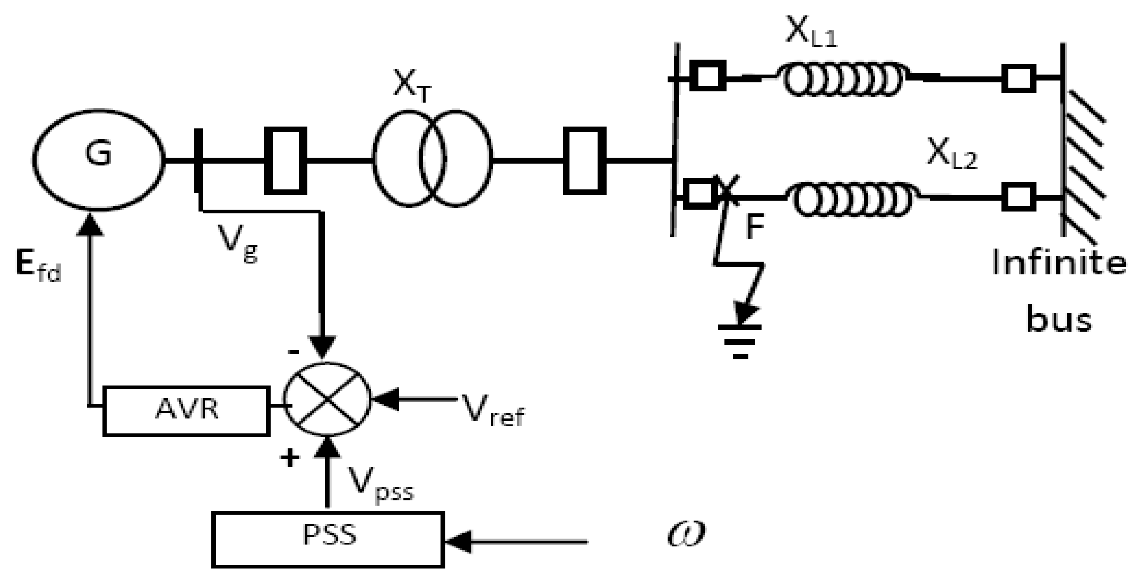
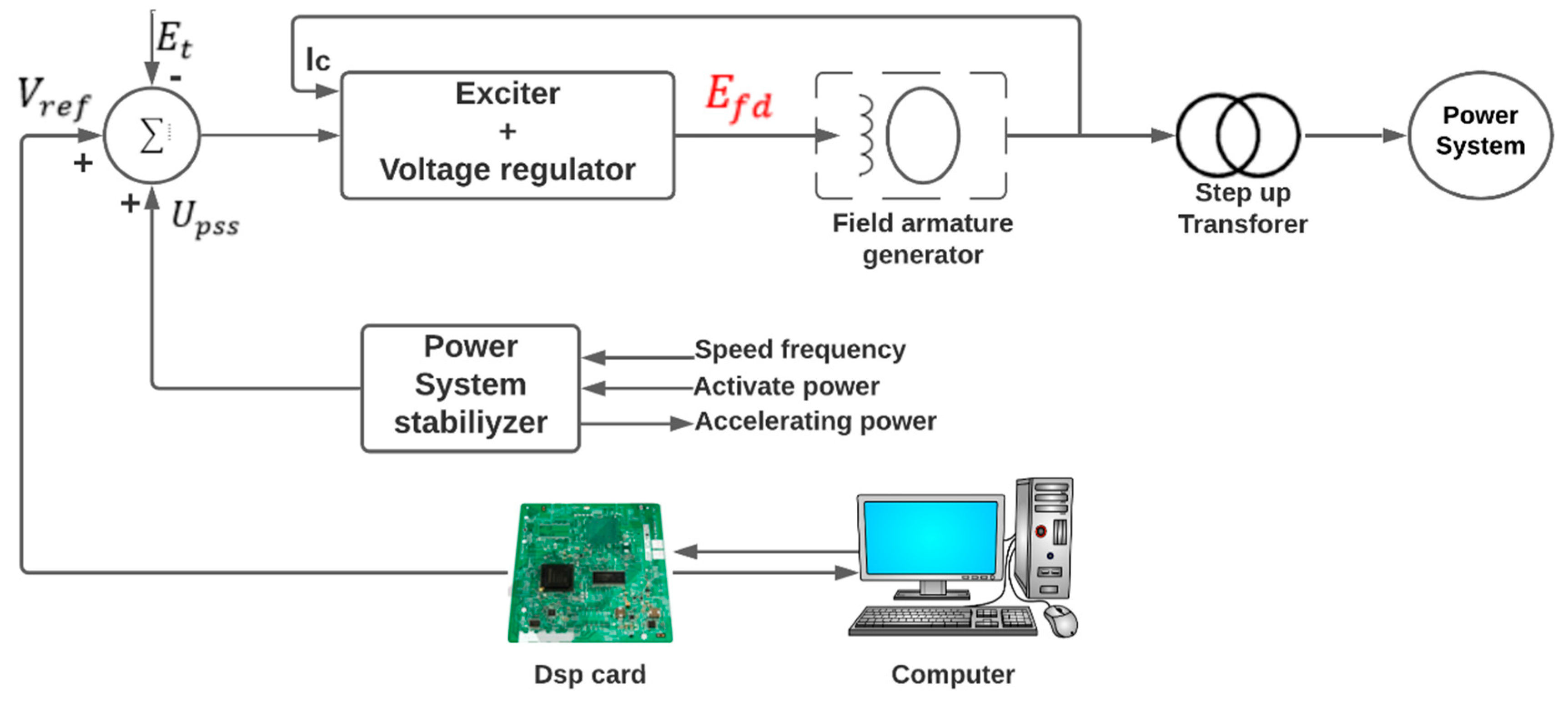
2.1. Power Network Modeling

A power system consisting of a synchronous generator with AVR and PSS controllers and connected through transmission lines to a very large network that can be approximated by an infinite bus, was considered in this study. A schematic diagram of the studied power system is shown in Figure 1.
The equations describing a third-order model of synchronous generators with the excitation system AVR can be written as [10,12]:
{ d δ d t = ω d ω d t = 1 2 H ( P m K D ω V B X d s E q sin δ + V B 2 ( X q X d ) 2 X d s X q s sin 2 δ d E q d t = 1 T d 0 ( E f d X d s X d s E q + X d X d X d s V B cos δ ) ) d E f d d t = 1 T a ( K a ( V r é f ( X q V B sin δ X q s ) 2 + ( X s X d s E q + X d X d s V B cos δ ) 2 + V p s s ) E f d )
with
{ X d s = X T + X L + X d X q s = X T + X L + X q X d s = X T + X L + X d
Figure 2 shows the interconnection between the PSS and AVR controller.
The mathematical model of the PSS controller is written as [10,11]:
{ d V 1 d t = 1 T ω ( K ω ω + V 1 ) d V 2 d t = 1 T 2 ( ( 1 T 1 T 2 ) ( K ω ω + V 1 ) V 2 ) d V 3 d t = 1 T 4 ( ( 1 T 3 T 4 ) ( V 2 + ( T 1 T 2 ( K ω ω + V 1 ) ) V 3 ) d V p s s d t = 1 T E ( V 3 + T 3 T 4 ( V 2 + T 1 T 2 ( K ω ω + V 1 ) ) V p s s )
In the state-space form, by combining Equations (1) and (2), we obtain a nonlinear mathematical model of the SMIB power system with the following form [10,11]:
{ d δ d t = ω d ω d t = a 1 ω a 2 E q sin δ + a 3 δ sin 2 δ 2 δ + a 4 P m d E q d t = a 5 δ cos δ δ a 6 E q + a 7 E f d d E f d d t = 1 T a ( K a ( V r é f δ ( K 1 sin δ δ ) 2 + ( K 2 E q + K 3 cos δ δ ) 2 + V p s s ) E f d ) d V 1 d t = a 8 ω 1 T ω V 1 d V 2 d t = a 9 ω + a 10 V 1 1 T 2 V 2 d V 3 d t = a 11 ω + a 12 V 1 + a 13 V 2 1 T 4 V 3 d V p s s d t = a 14 ω + a 15 V 1 + a 16 V 2 + 1 T E V 3 1 T E V p s s
with:
{ a 1 = K D 2 × H , a 2 = 1 2 H × X d s V B , a 3 = X d X d H X q s X d s V B 2 , a 4 = 1 2 H a 5 = X d X d T d 0 X d s V B , a 6 = 1 T d 0 X d s X d s , a 7 = 1 T d 0 , a 8 = K ω T ω , a 9 = ( 1 T 1 T 2 ) K ω T 2 a 10 = ( 1 T 1 T 2 ) 1 T 2 , a 11 = ( 1 T 3 T 4 ) T 1 T 2 K ω T 4 , a 12 = ( 1 T 3 T 4 ) T 1 T 2 1 T 4 , a 13 = ( 1 T 3 T 4 ) 1 T 4 a 14 = T 1 T 2 T 3 T 4 K ω T E , a 15 = T 1 T 2 T 3 T 4 1 T E , a 16 = T 3 T 4 1 T E K 1 = X q X q s V B , K 2 = X s X d s , K 3 = X d X d s V B X d s = X T + X L + X d , X q s = X T + X L + X q , X d s = X T + X L + X d
Let us consider the states of the power system X = [ x 1 x 2 x 3 x 4 x 5 x 6 x 7 x 8 ] T , where: x 1 = δ , x 2 = ω , x 3 = E q , x 4 = E f d , x 5 = V 1 , x 6 = V 2 , x 7 = V 3 and x 8 = V p s s , then: X = [ δ ω E q E f d V 1 V 2 V 3 V p s s ] T .
The objective of the control is to act on V r e f which affects directly the input E f d of the synchronous machine.
This complete model has four nonlinearities. To deal with this model we applied the T-S fuzzy technique. The T-S fuzzy model of the power system, also used for the design of the proposed controller, would be described in the next section.

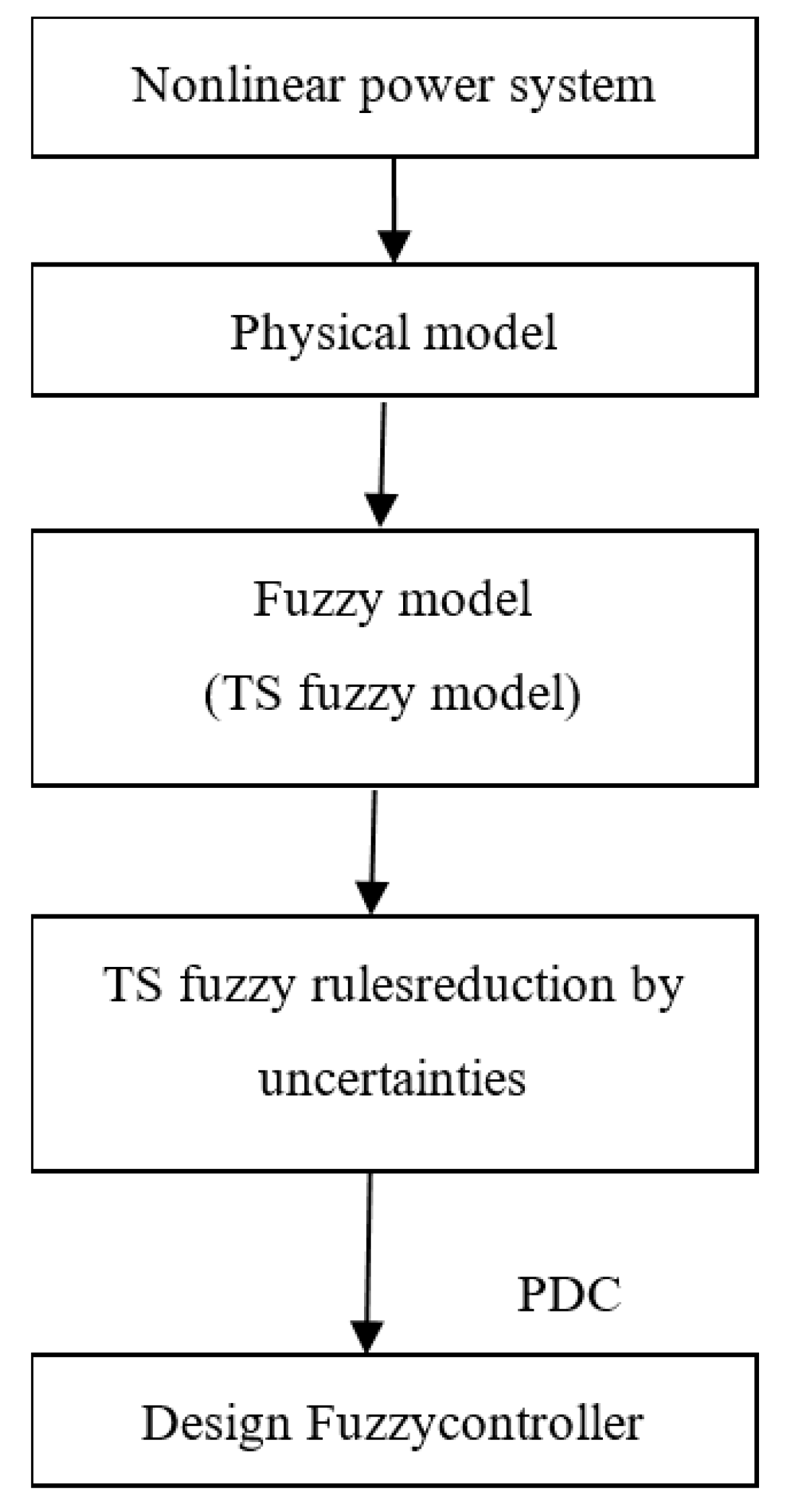
2.2. Fuzzy Model Stabilization

2.2.1. T-S Fuzzy Model

Let us consider a dynamic system described by:
X ( t ) = f ( X ( t ) , U ( t ) )
where f is the nonlinear function, X(t) is the state vector and U(t) is the input vector.
The main idea of this method was to describe the model (4) by a finite number of linear subsystems.
To obtain a T-S model, we can use the following [13]:
Lemma 1.
For x [ a , b ] , a > 0 and b > 0 either f ( x ) : a bounded function, then there are always two functions h 1 ( x ) : , h 2 ( x ) : and two scalars α and β satisfying the following properties h 1 ( x ) + h 2 ( x ) = 1 , h 1 ( x ) > 0 , h 1 ( x ) > 0 , h 2 ( x ) > 0 and f ( x ) = α h 1 ( x ) + β h 2 ( x ) .
Where:
h 1 ( x ) = f ( x ) f min f max f min ,   h 2 ( x ) = f max f ( x ) f max f min ,   α = f max   and   β = f min
Then, the T-S fuzzy rule is written [14,15,16,17,18,19]:
R i :   if   Z 1   is   F 1 i ( z 1 ( t ) )   and   Z p   is   F p i ( z p ( t ) )
Then:
X ( t ) = i = 1 r w i ( Z ( t ) ) { A i X ( t ) + B i U ( t ) } i = 1 r w i ( Z ( t ) ) = i = 1 r h i ( Z ( t ) ) { A i X ( t ) + B i U ( t ) }
where w i ( Z ( t ) ) is a weight,
{ w i ( Z ( t ) ) = j = 1 p F j i ( Z ( t ) ) t w i ( Z ( t ) ) 0 ; i = 1 , 2 , , r h i ( Z ( t ) ) = w i ( Z ( t ) ) i = 1 r w i ( Z ( t ) ) , i = 1 r h i ( Z ( t ) ) = 1
Then, the linear TS system is described as follow:
X ( t ) = A z X ( t ) + B z U ( t )
with { A z = h i ( Z ( t ) ) A i B z = h i ( Z ( t ) ) B i .

2.2.2. PDC Fuzzy Controller Design

The PDC offers a procedure to design a fuzzy controller from a given T-S fuzzy model. To achieve the PDC law, a controlled object (nonlinear system) was first represented by a T-S fuzzy model. In the PDC design, each control rule was designed from the T-S fuzzy model corresponding rule.
A PDC controller, for this T-S model, was defined as follows [20]:
U ( t ) = i = 1 r h i ( Z ( t ) ) F i X ( t ) = F z X ( t )
The control law was obtained by calculating the F i . Then, for a continuous system, a quadratic Lyapunov function was considered [20]:
V ( x ( t ) ) = x T ( t ) P x ( t )
with:
{ P > 0 V ( x ) < 0
This led to LMI conditions that had to be solved to determine the feedback gains [13].
Lets use:
X A Z T + A Z X M Z T B Z T B Z M Z < 0
with: { X = P 1 F i = M i P 1 .
Equation (10) is verified if [21,22]:
i , ϒ i i < 0
i , j ,   i < j ,   ϒ i j + ϒ j i < 0
ϒ i j = X A i T + A i X i T B j M i M i T B j T < 0
These LMIs conditions are very conservative. To reduce this conservativeness, some lemmas are used:
Lemma 2.
Matrices X ,   Y   and   R being of appropriate sizes such that [13,23]:
{ Y X R 1 X T > 0 R > 0 [ Y X T ( * ) R ]
(*) represents all terms induced by symmetry in a symmetric matrix.
Lemma 3.
The two next problems are equivalent [21,23]:
(i) 
Find P > 0 , such that:
T + A T P + P A < 0
(ii) 
Find P > 0 ,   L ,   G such that:
[ T + A T L + L A P L + G T A ( * ) G G T ] < 0
Lemma 4.
Let the matrices ϒ i j and the condition be [4,21]:
ϒ z z = i = 1 r h i 2 ( z ) ϒ i i + i = 1 r i = 1 r h i ( z ) h j ( z ) ( ϒ i j + ϒ j i ) < 0
Equation (16) is verified if there are Q i and Q i j , ( i > j ) such that the following conditions are respected:
i ,   ϒ i i < Q i i
i , j ,   i < j ,   ϒ i j + ϒ j i < Q i j + Q j i
[ Q 11 Q 21 Q r 1 Q 22 Q r ( r 1 ) ( * ) Q r r ] < 0
With the increase in the number of nonlinearities in the model, we obtain an important number of LMIs conditions that the solver cannot find feasible solutions. In this regard, it is important to decrease the number of nonlinearities and get a minimum number of fuzzy rules. To this end, a TS fuzzy rules reduction by uncertainties was proposed.

2.3. TS Fuzzy Rules Reduction by Uncertainties

2.3.1. Uncertain TS Fuzzy Model

This technique is based on considering some nonlinearities as uncertainties in the system model [16,21,24,25,26,27].
Then, the system (5) becomes of the following form:
X ( t ) = r = 1 r h i { ( A i + Δ A i ) X ( t ) + ( B i + Δ B i ) U ( t ) }
with:
Δ A i = H a Δ a i E a i ,   Δ B i = H b Δ b i E b i
where H a ,   H b ,   E a i ,   E b i are constant matrices and:
Δ a i Δ a i T < 1 ,   Δ b i Δ b i T < 1
System (21) can also be written in the following form:
X ( t ) = ( A z + Δ A z ) X ( t ) + ( B z + Δ B z ) U ( t )
Let be a nonlinear function α ( t ) [   α min   α max ] , then:
α i ( t ) = α i m + β ( t ) α i r ,   i = 1 n
where:
n: is number of uncertainties
{ α i m = 0 , 5 ( α i max + α i min ) α i r = 0 , 5 ( α i max α i min ) ,   β ( t ) [ 1 1 ]

2.3.2. System Stability and Robustness with Uncertainties

We considered a Lyapunov quadratic function [21]: V ( x ) = x T P x .
To guarantee the stability of the system the decay rate δ was selected, so we had to have [21]:
V ( x ) < 2 δ V ( x )
Using the fact that [21]:
λ min ( P ) x ( t ) 2 V ( x ( t ) ) = x T ( t ) P x ( t ) λ max ( P ) x ( t ) 2
λ ( . ) min and λ ( . ) max are respectively small and large eigenvalues.
So,
x ( t ) 1 λ ( P ) min 1 / 2 λ ( P ) max 1 / 2 x ( 0 ) e δ t
λ ( P ) min x ( t ) 2 V ( x ( 0 ) ) e 2 δ t λ ( P ) max x ( 0 ) 2 e 2 δ t
x ( t ) λ ( P ) max 1 / 2 λ ( P ) min 1 / 2 x ( 0 ) e δ t
For all the initial conditions x ( 0 )
Inserting Equation (8) in (22), the closed-loop can be written as:
X ( t ) = ( A z B z F z + Δ A z Δ B z F z ) X ( t )
Equation (9) corresponds to:
X T { ( A z B z F z + Δ A z Δ B z F z ) T P + P ( A z B z F z + Δ A z Δ B z F z ) + 2 δ P } X < 0
Using the after, pre, and post multiplication by X = P 1 with M z = F z P 1 , the Equation (32) becomes:
X A z T + A z X M z T B z T B z M z + X Δ A z T + Δ A z X M z T Δ B z Δ B z M z + 2 δ X < 0
with
{ Δ A z = H Δ a z ( t ) E a z Δ B z = H Δ b z ( t ) E b z
Then,
X A z T + A z X M z B z T B z M z + 2 δ X + X E a z T Δ a z T H T + H Δ a z E a z X X E b z T Δ b z T H T + H Δ b z E b z X < 0
By considering the following property [21]:
X T Y + Y T X τ X T X + τ 1 Y T Y   and   τ > 0
with τ a z > 0 and τ b z > 0 .
Then Equation (35) would be written in the following form:
{ X A z T + A z X M z B z T B z M z + 2 δ X + τ a z 1 X E a z T Δ a z T Δ a z E a z X + τ a z H H T + τ b z 1 X E b z T Δ b z T Δ b z E b z X + τ b z H H T < 0
By construction: Δ a z T Δ a z I and Δ b z T Δ b z I , Equation (36) is established if:
{ X A z T + A z X M z B z T B z M z + 2 δ X + τ a z 1 X E a z T E a z X + τ a z H H T + τ b z 1 X E b z T E b z X + τ b z H H T < 0
or equivalently:
{ X A z T + A z X M z B z T B z M z + 2 δ X + X E a z T τ a z 1 E a z X + τ a z H τ a z 1 H T τ a z + X E b z T τ b z 1 E b z X + τ b z H τ b z 1 H T τ b z < 0
The use of Lemma 2 gives:
[ X A i T + A i X i T B j M i M i T B j T + 2 δ X τ a z H X E a z T τ b z H M z T E b z T τ a z H T τ a z I 0 0 0 E a z X 0 τ a z I 0 0 τ b z H T 0 0 τ b z I 0 E b z M z 0 0 0 τ b z I ] < 0
For a robust stabilization, the used LMI condition is [21]:
ϒ i j = [ X A i T + A i X i T B j M i M i T B j T + 2 δ X τ a i H X E a i T τ b i H M j T E b i T τ a i H T τ a i I 0 0 0 E a i X 0 τ a i I 0 0 τ b i H T 0 0 τ b i I 0 E b i M j 0 0 0 τ b i I ] < 0
Theorem 1.
Assuming the uncertain TS model (24), the PDC law (8) and the ϒ i j (13), if there exists a matrix X > 0 , a scalar τ a i > 0 , τ b i > 0 , matrices M i ,   Q i i ,   Q i j ,   i , j { 1 , , r } ,   i < j such that conditions (18), (19) and (20) are verified, then the closed-loop is globally exponentially stable [20].
Figure 3 illustrates the model-based fuzzy control design approach discussed in this paper. To design a fuzzy controller, we need a TS fuzzy model for a nonlinear system. Therefore, the construction of fuzzy models represented an important and basic procedure in this approach.

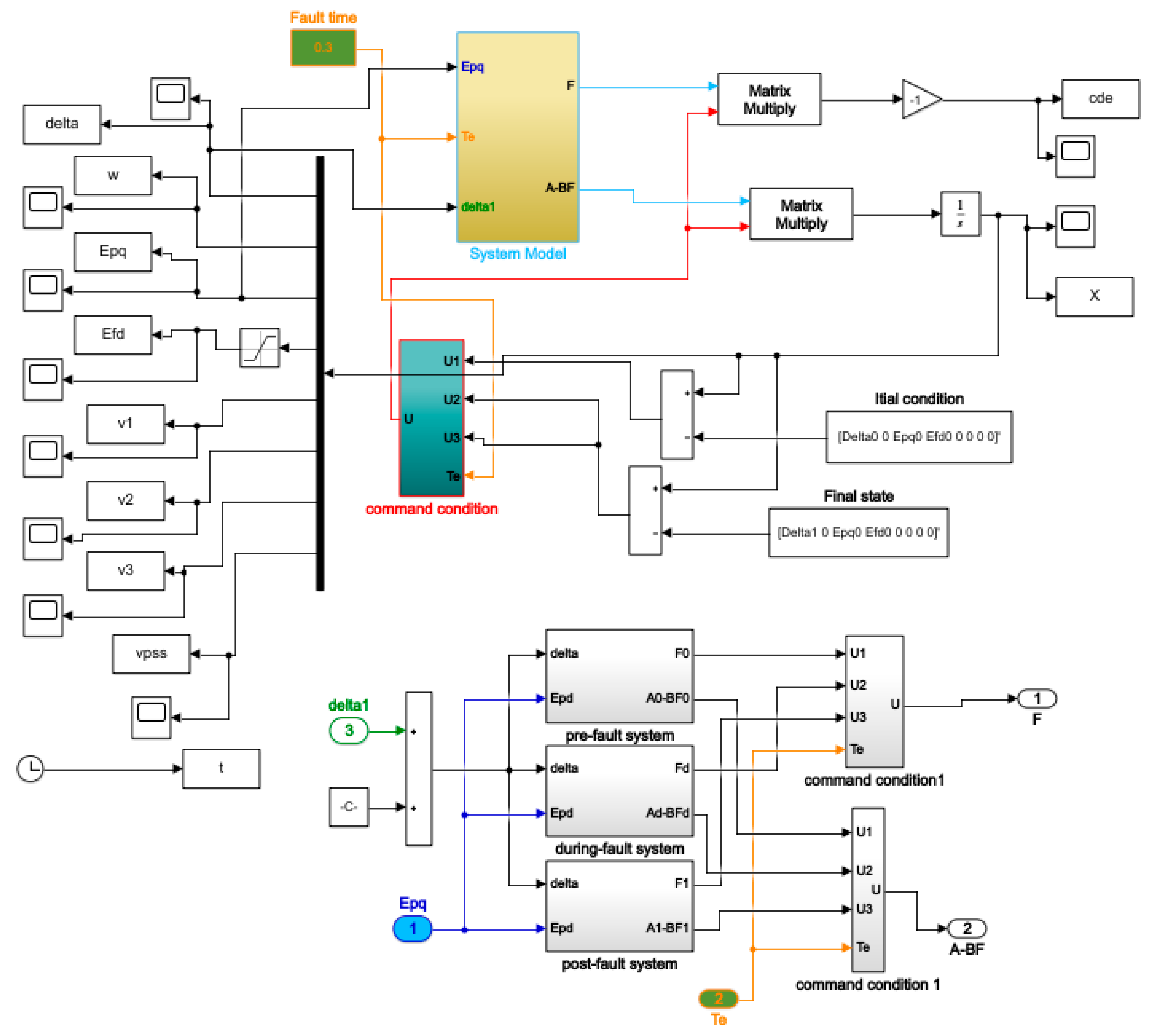
2.4. Application: Stabilization of SMIB Power System by T-S Fuzzy PDC Controller

2.4.1. System Test

The proposed controller is tested on a power system presented in Figure 1. The objective of this section was to design a robust controller in order to ensure that all signals in the closed-loop system reached the desired state. As perturbation, the power system is affected by an unexpected default at line transmission X L 2 during the time t f .
So, three states (pre-fault, during fault, post-fault) were presented with [11]:
X L = { X L 1 X L 2   p r e - f a u l t   s t a t e   t < t 1 = 1 s 0   d u r i n g   f a u l t   s t a t e   t 1 < t < t 2 = t 1 + t f X L 1   p o s t - f a u l t   s t a t e   t > t 2
In this work, the objective was to control the voltage reference V r e f , which affects directly the voltage excitation E f d of the synchronous machine, calculated in the three states (pre-fault, during fault, post-fault). Then, the global control law would be as follows:
V r e f = { V r e f ( p r e - f a u l t )   at   t < t 1 = 1 s V r e f ( d u r i n g - f a u l t )   at   t 1 < t < t 2 = t 1 + t f V r e f ( p o s t - f a u l t )   at   t > t 2

2.4.2. Construction of T-S Fuzzy Model for SMIB Power System

According to the system Equation (4), there are 4 nonlinearities:
z 1 = ( K 1 sin ( δ ) δ ) 2 + ( K 2 E q δ + K 3 cos ( δ ) δ ) 2
z 2 = sin ( δ )
z 3 = sin ( 2 δ ) 2 δ
z 4 = cos ( δ ) δ
That leads to 24 = 16 linear models.
Then the fuzzy system has the state-space form:
  X ( t ) = i = 1 16 h i ( z ( t ) ) ( A i X ( t ) + B i u ( t ) )
The pair ( A 1 , B 1 ) for the first model can be written as follows:
A 1 = [ 0 1 0 0 0 0 0 0 2 a 3 z 2 max a 1 a 2 z 1 max 0 0 0 0 0 a 5 z 3 max 0 a 6 a 7 0 0 0 0 K a T a z 4 max 0 0 1 T a 0 0 0 K a T a 0 a 8 0 0 1 T ω 0 0 0 0 a 9 0 0 a 10 1 T 2 0 0 0 a 11 0 0 a 12 a 13 1 T 4 0 0 a 14 0 0 a 15 a 16 1 T E 1 T E ]
B = [ 0 0 0 K a T a 0 0 0 0 ]
The other 15 models, having the same form as the first, are obtained by permuting z i max and z i min , for i = 1 4 . In this case, it is difficult to find the feedback gains of the controller because the number of LMI conditions is important. Then, the solver cannot get a solution to this problem. To avoid the exponential increase in the rules number related to the nonlinear functions, the T-S model with uncertainties is proposed and developed.

2.4.3. Nonlinearities Reduction by Uncertainties

This method consists of considering some nonlinearities as uncertainties. Then the fuzzy model obtained contains less number of rules that can facilitate the resolution of LMI conditions.
To our knowledge, there is no systematic method for the choice of the nonlinearities considered in the uncertainties (number and choice of non-linearities) related to the dynamics of the system. To meet this challenge, we tried several combinations concerning the number of nonlinearities. For example, we treated the case of two nonlinearities in the simulation and results section. The best result was given by the choice of a single nonlinearity Z1 and the others were considered as uncertainties.
Then we considered a single nonlinearity:
z 1 = ( K 1 sin ( δ ) δ ) 2 + ( K 2 E q δ + K 3 cos ( δ ) δ ) 2
Using Lemma 1, Z1 can be written in the following form:
z 1 ( t ) = z 1 ( t ) z 1 min z 1 max z 1 min z 1 max + z 1 max z 1 ( t ) z 1 max z 1 min z 1 min = h 1 1 ( t ) z 1 max + h 1 2 ( t ) z 1 min
with { { z 1 max 0 = ( K 10 ) 2 + ( K 20 E q 0 ε + K 30 ε ) 2 z 1 min 0 = ( K 10 2 π ) 2 + ( 2 K 20 E q r π + 2 K 30 ε π ) 2   at   t < t 1 = 1 s { z 1 max d = ( K 1 d ) 2 + ( K 2 d E q 0 ε + K 3 d ε ) 2 z 1 min d = ( K 1 d 2 π ) 2 + ( 2 K 2 d E q r π + 2 K 3 d ε π ) 2   at   t 1 < t 1 < t 2 { z 1 max 1 = ( K 11 ) 2 + ( K 21 E q 0 ε + K 31 ε ) 2 z 1 min 1 = ( K 11 2 π ) 2 + ( 2 K 21 E q r π + 2 K 31 ε π ) 2   at   t > t 2 and E q r < E q < E q 0 .
The 3 other nonlinearities were transformed into uncertainties using Expression (25).
For the firstnonlinearities α 1 ( t ) = sin ( δ ) we can write with β ( t ) = 1 : α 1 ( t ) = α 1 m + β ( t ) α 1 r , where:
{ α 1 m = 0.5 × ( α 1 max + α 1 min ) α 1 r = 0.5 × ( α 1 max α 1 min )   and   { α 1 max = ε α 1 min = 1
For the second nonlinearities   α 2 ( t ) = sin ( 2 δ ) 2 δ we can write with β ( t ) = 1 : α 2 ( t ) = α 2 m + β ( t ) α 2 r , where:
{ α 2 m = 0.5 × ( α 2 max + α 2 min ) α 2 r = 0.5 × ( α 2 max α 2 min )   and   { α 2 max = 2 ε π α 2 min = 1
For the third nonlinearities   α 3 ( t ) = cos ( δ ) δ we can write with β ( t ) = 1 : α 3 ( t ) = α 3 m + β ( t ) α 3 r , where:
{ α 3 m = 0.5 × ( α 3 max + α 3 min ) α 3 r = 0.5 × ( α 3 max α 3 min )   and   { α 3 max = 2 ε π α 3 min = 1 ε
Using a single nonlinearity, two rules were obtained, the model is:
X ( t ) = i = 1 2 h i { ( A i + Δ A i ) X ( t ) + B U ( t ) }
For example, The T-S fuzzy model of the pre-fault state is constructed as follows:
  • Rule 1. R 1 : if z 1 is h 10 1 . Then   X = ( A 1 + Δ A 1 ) X + B 1 U .
  • Rule 2. R 2 : if z 1 is h 10 2 . Then   X = ( A 2 + Δ A 2 ) X + B 2 U , where:
    A 1 = ( 0 1 0 0 0 0 0 0 α 2 m a 1 α 1 m 0 0 0 0 0 α 3 m 0 a 6 a 7 0 0 0 0 K a T a z 1 max 0 0 0 1 T a 0 0 0 K a T a 0 a 8 0 0 1 T ω 0 0 0 0 a 9 0 0 a 10 1 T 2 0 0 0 a 11 0 0 a 12 a 13 1 T 4 0 0 a 14 0 0 a 15 a 16 1 T E 1 T E )
    Δ A 1 = ( 0           0 α 2 r 0 α 1 r           α 3 r 0         0                                                       0       0 )
    A 2 = ( 0 1 0 0 0 0 0 0 α 2 m a 1 α 1 m 0 0 0 0 0 α 3 m 0 a 6 a 7 0 0 0 0 K a T a z 1 min 0 0 0 1 T a 0 0 0 K a T a 0 a 8 0 0 1 T ω 0 0 0 0 a 9 0 0 a 10 1 T 2 0 0 0 a 11 0 0 a 12 a 13 1 T 4 0 0 a 14 0 0 a 15 a 16 1 T E 1 T E )
    Δ A 2 = ( 0           0 α 2 r 0 α 1 r           α 3 r 0         0                                                       0       0 )
The input matrices B 1 and B 2 are:
B 1 = B 2 = B = [ 0 0 0 K a T a 0 0 0 0 ]
From Expression (22) of uncertainties;
Δ A 1 = Δ A 2 = H a Δ a ( t ) E a
with:
E a = ( 0           0 α 2 r 0 α 1 r           α 3 r 0         0                                                       0       0 )
H a = ( 0           0 1 0             0 1 0             0 0                                                   0         0 )
Δ a = ( 0           0 1 0             0 1 0             0 0                                                   0         0 )
B is a constant vector then:
Δ B 1 = Δ B 2 = H b Δ b ( t ) E b = 0
In the next sub-section, the proposed approach using the T-S model with uncertainties was compared with the Taylor linearization method to prove the efficiency of this approach.

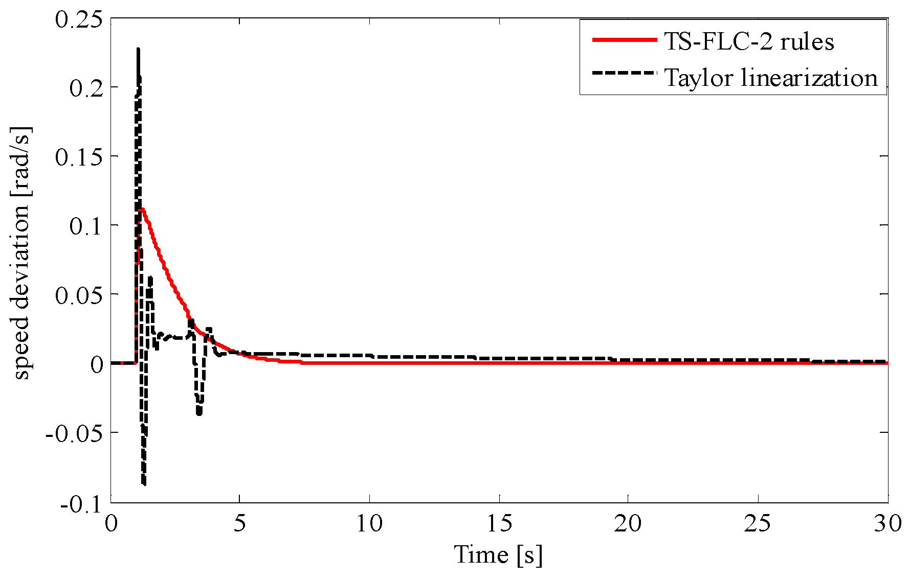
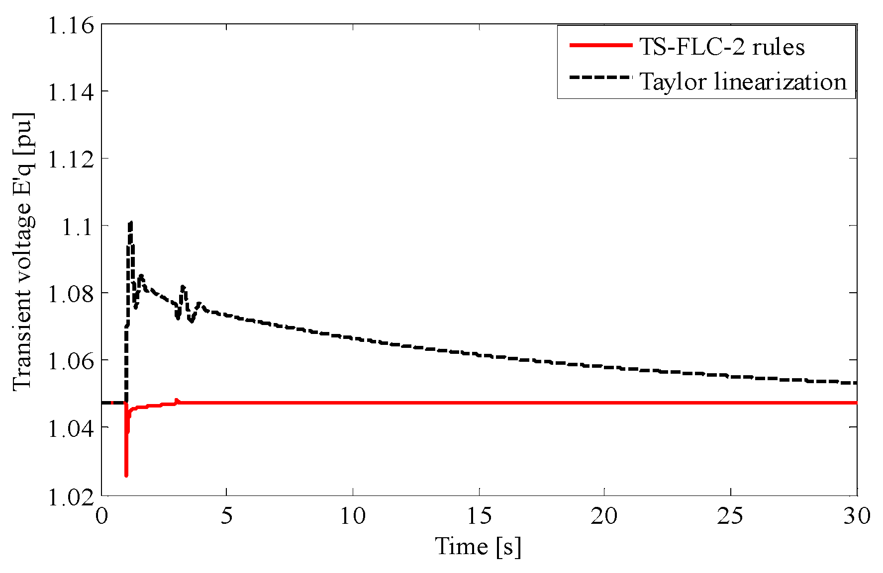
2.4.4. Taylor Linearization

For the system X = f ( X i , U i ) , the Taylor series can be expressed as follows:
f ( X i , U i ) = f ( X s i , U s i ) 0   in   steady   flow + f X i | X s i , U s i ( X i X s i ) + f U i | X s i , U s i ( U i U s i )
Then, this Taylor series was applied to system (4) for the three states:
  • Pre-fault state:
    { δ = f ( ω ) = f ω | ω 0 ω ω = f ( δ , ω , E p q ) = f δ | δ 0 , ω 0 , E p q 0 δ + f ω | δ 0 , ω 0 , E p q 0 ω + f E p q | δ 0 , ω 0 , E p q 0 E p q = a 2 cos ( δ 0 ) E p q 0 δ a 2 sin ( δ 0 ) E p q + 2 a 3 cos ( 2 δ 0 ) δ + a 1 ω E p q = f ( δ , E p q , E f d ) = a 5 sin ( δ 0 ) δ + a 6 E p q + a 7 E f d E f d = f ( δ , E p q , E f d , V p s s , U ) = 1 T A { K A [ V r e f ( 2 ( K 10 cos ( δ 0 ) sin ( δ 0 ) 2 K 30 sin ( δ 0 ) cos ( δ 0 ) + 2 K 20 K 30 E p q 0 sin ( δ 0 ) 2 ( K 10 sin ( δ 0 ) ) 2 + ( K 20 E p q 0 + K 30 cos ( δ 0 ) ) 2 f 10 δ 2 ( K 10 K 30 cos ( δ 0 ) + K 20 E p q 0 2 ( K 10 sin ( δ 0 ) ) 2 + ( K 20 E p q 0 + K 30 cos ( δ 0 ) ) 2 f 20 E p q ) + V p s s ] E f d } V 1 = a 8 ω + 1 T ω V 1 V 2 = a 9 ω + a 10 V 1 1 T 2 V 2 V 3 = a 11 ω + a 12 V 1 + a 13 V 2 1 T 4 V 3 V p s s = a 14 ω + a 15 V 1 + a 16 V 2 + 1 T E V 3 1 T E V p s s
    with
    { δ = δ δ 0 , ω = ω ω 0 , E p q = E p q E p q 0 , E f d = E f d E f d 0 , V 1 = V 1 V 10 , V 2 = V 2 V 20 , V 3 = V 3 V 30 , V p s s = V p s s V p s s 0
    A 0 = ( 0 1 0 0 0 0 0 0 a 2 cos ( δ 0 ) E q 0 + 2 a 3 cos ( 2 δ 0 ) a 1 a 2 sin ( δ 0 ) 0 0 0 0 0 a 5 sin ( δ 0 ) 0 a 6 a 7 0 0 0 0 K a T a f 10 0 K a T a f 20 1 T a 0 0 0 K a T a 0 a 8 0 0 1 T ω 0 0 0 0 a 9 0 0 a 10 1 T 2 0 0 0 a 11 0 0 a 12 a 13 1 T 4 0 0 a 14 0 0 a 15 a 16 1 T E 1 T E )
  • During fault state:
    The equilibrium point during the fault is the same after the fault elimination. Then,
    A d = ( 0 1 0 0 0 0 0 0 a 2 cos ( δ d ) E q d + 2 a 3 cos ( 2 δ d ) a 1 a 2 sin ( δ d ) 0 0 0 0 0 a 5 sin ( δ d ) 0 a 6 a 7 0 0 0 0 K a T a f 1 d 0 K a T a f 2 d 1 T a 0 0 0 K a T a 0 a 8 0 0 1 T ω 0 0 0 0 a 9 0 0 a 10 1 T 2 0 0 0 a 11 0 0 a 12 a 13 1 T 4 0 0 a 14 0 0 a 15 a 16 1 T E 1 T E )
    with
    { δ = δ δ 1 , ω = ω ω 1 , E p q = E p q E p q 1 , E f d = E f d E f d 1 , V 1 = V 1 V 11 , V 2 = V 2 V 21 , V 3 = V 3 V 31 , V p s s = V p s s V p s s 1
    { f 1 d = 2 ( K 1 d cos ( δ d ) sin ( δ d ) 2 K 3 d sin ( δ d ) cos ( δ d ) + 2 K 2 d K 3 d E p q d sin ( δ d ) 2 ( K 1 d sin ( δ d ) ) 2 + ( K 2 d E p q d + K 3 d cos ( δ d ) ) 2 f 2 d = 2 ( K 1 d K 3 d cos ( δ d ) + K 2 d E p q d 2 ( K 1 d sin ( δ d ) ) 2 + ( K 2 d E p q d + K 3 d cos ( δ d ) ) 2
  • Post-fault state:
    A 1 = ( 0 1 0 0 0 0 0 0 a 2 cos ( δ d ) E q d + 2 a 3 cos ( 2 δ d ) a 1 a 2 sin ( δ d ) 0 0 0 0 0 a 5 sin ( δ d ) 0 a 6 a 7 0 0 0 0 K a T a f 11 0 K a T a f 21 1 T a 0 0 0 K a T a 0 a 8 0 0 1 T ω 0 0 0 0 a 9 0 0 a 10 1 T 2 0 0 0 a 11 0 0 a 12 a 13 1 T 4 0 0 a 14 0 0 a 15 a 16 1 T E 1 T E )
    with
    { f 11 = 2 ( K 11 cos ( δ d ) sin ( δ d ) 2 K 31 sin ( δ d ) cos ( δ d ) + 2 K 21 K 31 E p q d sin ( δ d ) 2 ( K 11 sin ( δ d ) ) 2 + ( K 21 E p q d + K 31 cos ( δ d ) ) 2 f 21 = 2 ( K 11 K 31 cos ( δ d ) + K 21 E p q d 2 ( K 11 sin ( δ d ) ) 2 + ( K 21 E p q d + K 31 cos ( δ d ) ) 2
    B = [ 0 0 0 K a T a 0 0 0 0 ]

3. Results

Simulation studies were conducted on the SMIB power system, presented in Figure 1, in order to check the performance of the proposed nonlinear control scheme. The model of the studied power system was built in MATLAB/SIMULINK environment as shown in Figure 4.
The system parameters given in Table 1 represent the data of the studied power system (synchronous machines constants, transmission line constants, PSS constants, AVR constants). The initial conditions of the state variables for the power system model, presented in Section 2, are computed by systematically solving the load flow program of the network first, and then computing the other algebraic and state variables given in Table 2. This program is based on the Newton–Raphson method [10].
The Critical Clearing Time (CCT) without regulator is tcc = 1.112 s. To prove the robustness of the proposed regulator, it was revealed that during fault time t f = 2 s is greater than tcc.
For simulations, the model rules were chosen for:
ε < δ < π 2 ε ,   ε = 0.1   and   E q r = 0.1 ,
The feedback gains of the Takagi–Sugeno Fuzzy Logic Controller (TS-FLC) were calculated by using the relaxed stability LMI conditions satisfying Theorem 1.

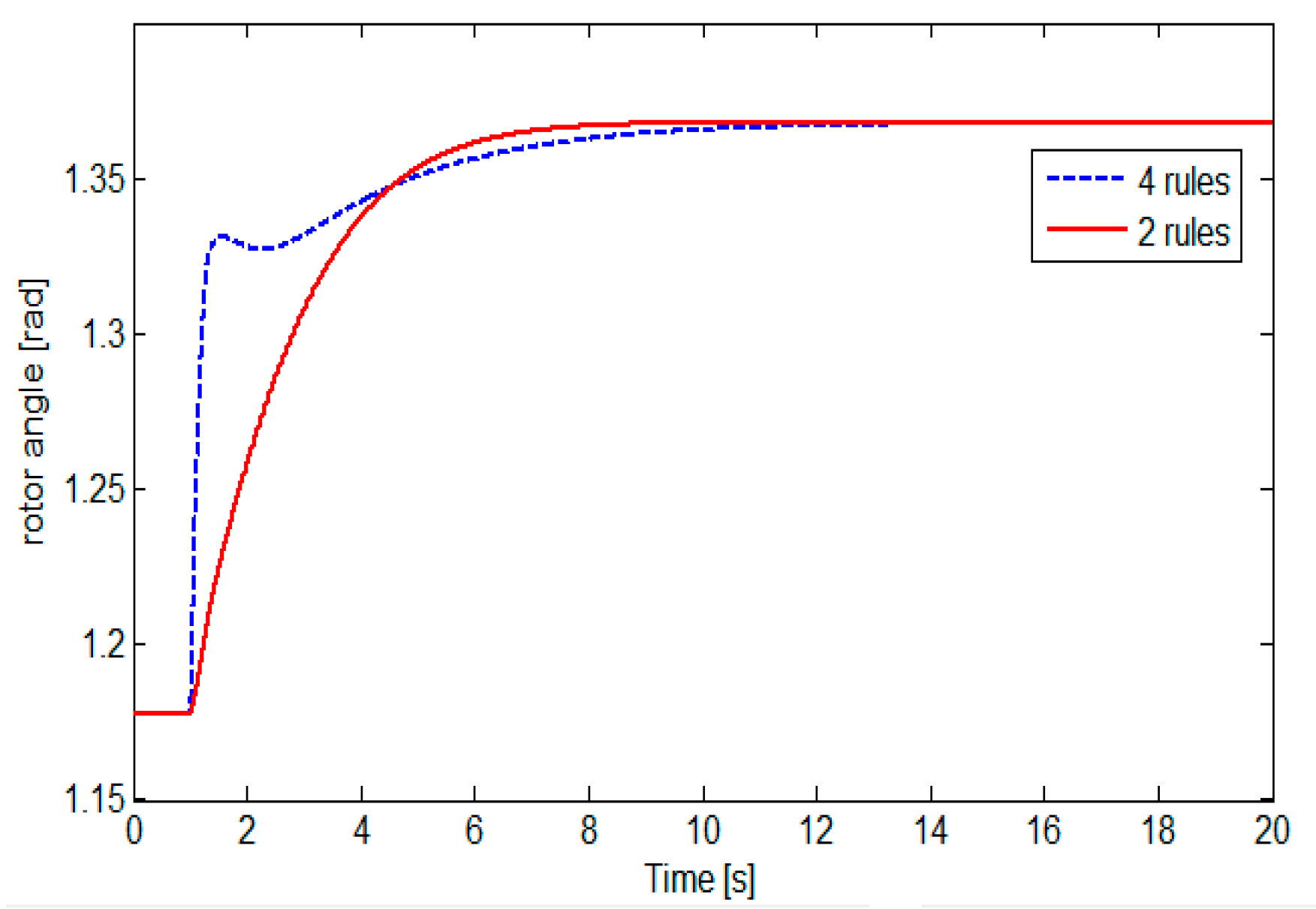
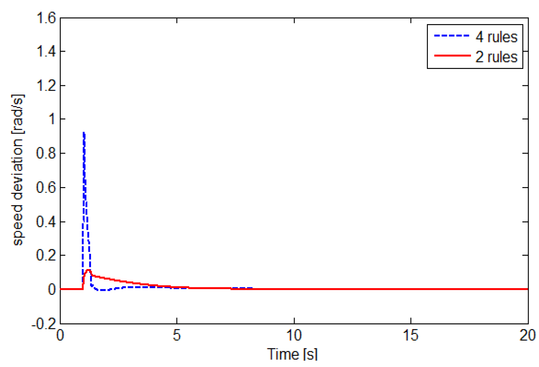
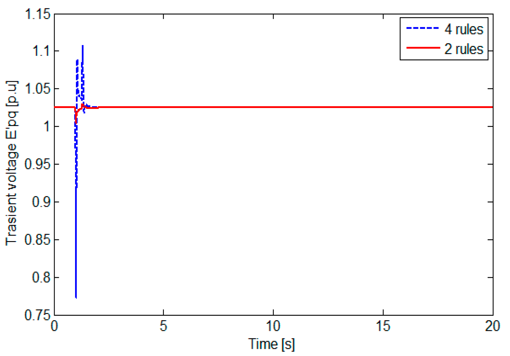
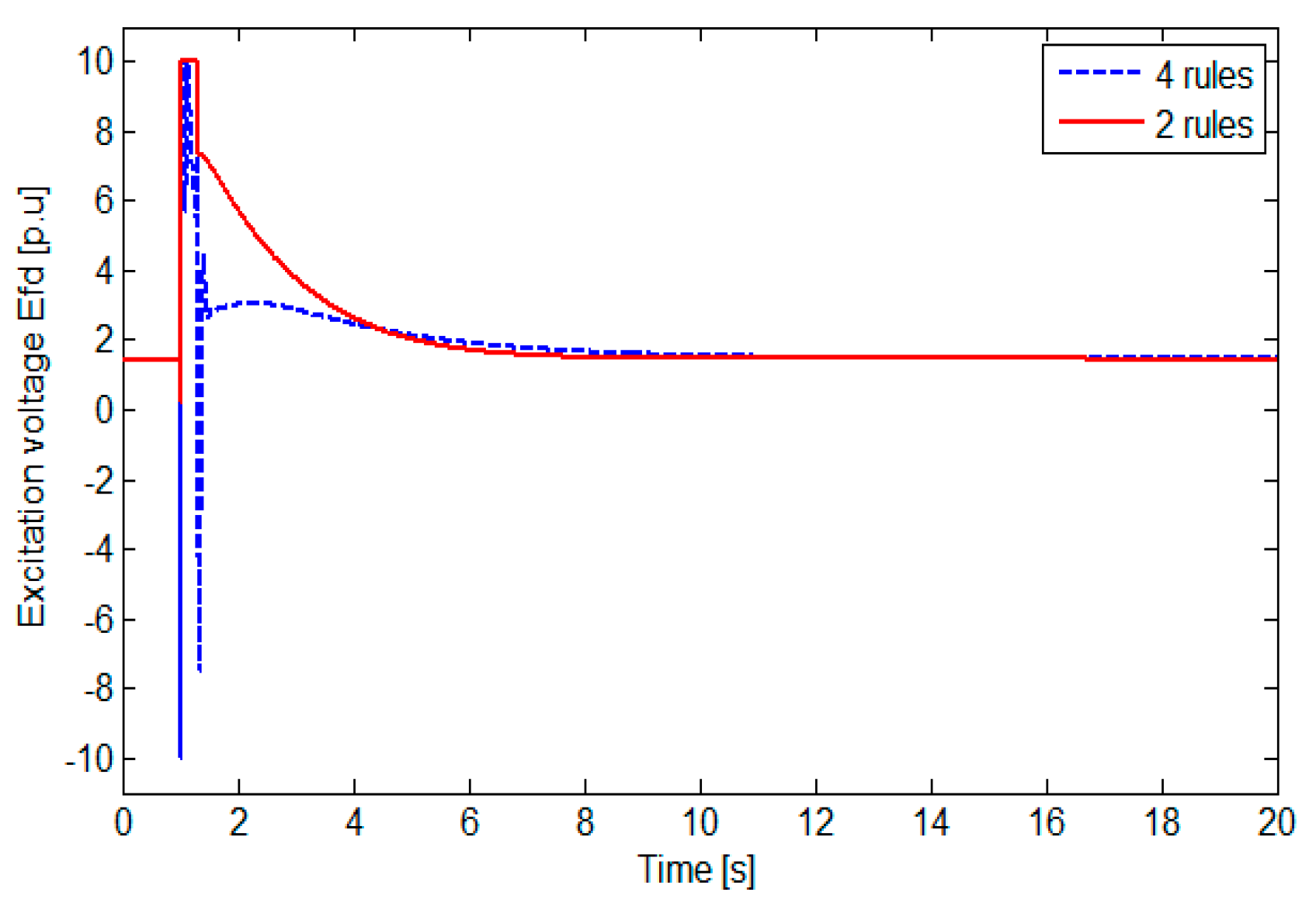
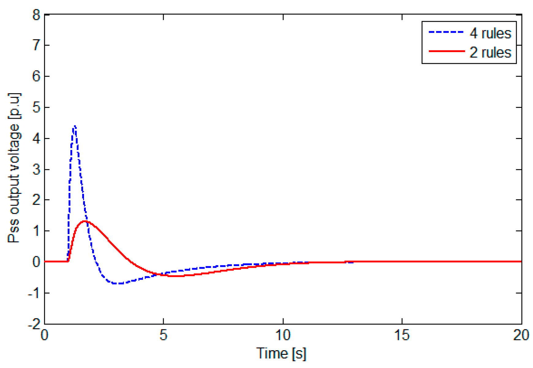
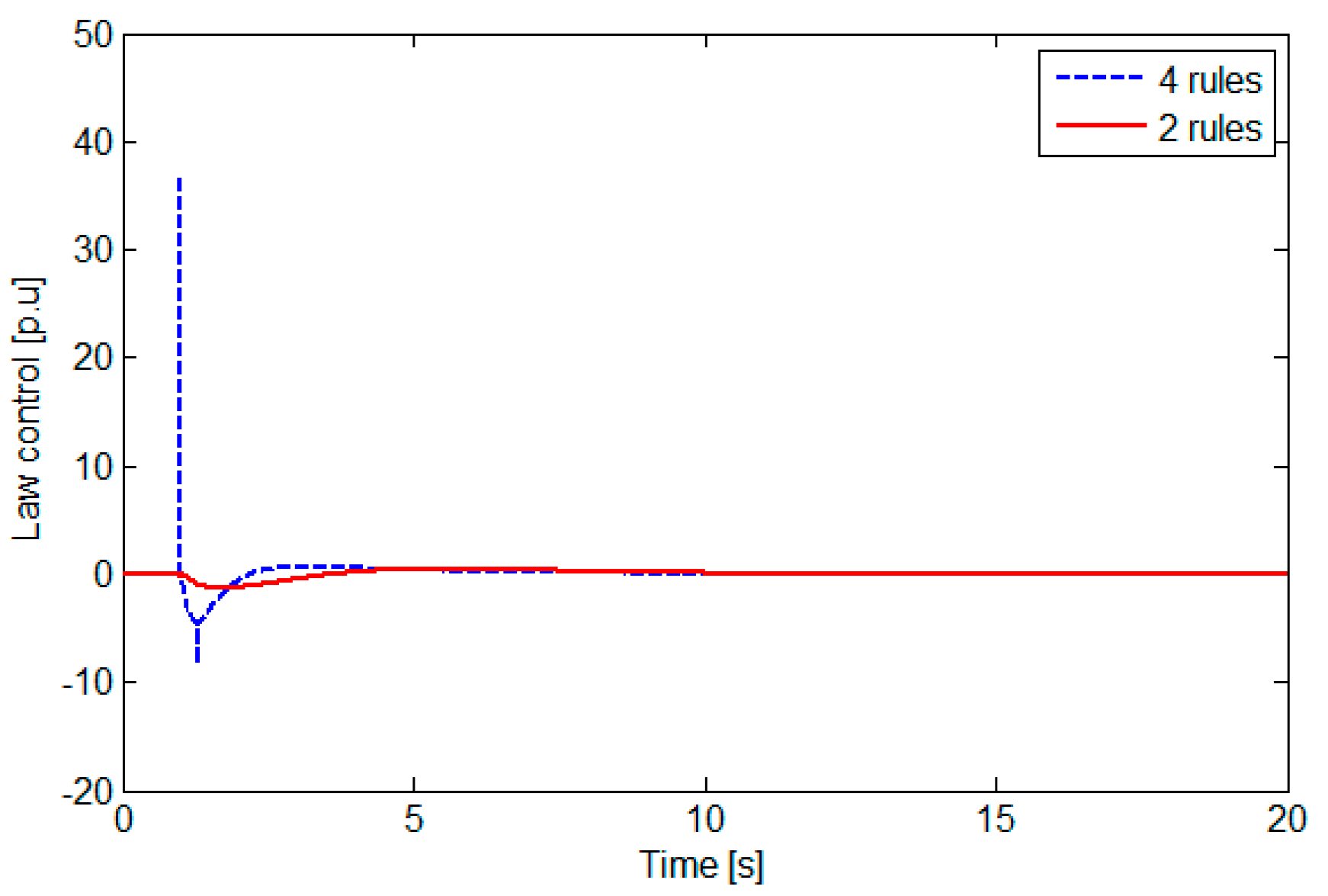
3.1. Comparison: One Nonlinearity (Two-Rule Model) and Two Nonlinearities (Four-Rule Model)

As said in Section 2.3, we performed many simulation tests for the choice of the linearities number considered in the system model. We presented, as an example, the case of one nonlinearity (two-rule model) and two nonlinearities (four-rule model).
The results shown in Figure 5, Figure 6, Figure 7, Figure 8 and Figure 9 illustrate the comparative studies between the two cases. The design of the regulators includes the study, analysis and verification of stability.
Figure 5 shows the variation of the rotor angle which starts from the initial value δ0 to the desired value δd calculated previously. When the fault is applied, at t = 1 s with a fault time tf = 2 s greater than the critical cleaning time tcc, we can clearly see a slight overshoot. Similarly for the variation of the speed deviation, presented in Figure 6, it can be seen that the disturbance generates a small peak value which is eliminated rapidly and the speed deviation tends towards the desired value.
Based on the voltage curves given by Figure 7, Figure 8 and Figure 9, there is a slight fluctuation in these voltages which remains stable during and after the disturbance.
In view of these results, it can be seen that the power system returns to the desired state within a few seconds after applying the fault in a critical situation (fault duration greater than the critical cleaning time). Even if the duration of the fault is further increased, the system regains its equilibrium point. This proves the robustness of the proposed controller.
Figure 10 shows the control law variation. It is clear that the two-rule model has a lower amplitude at fault application. In addition, this fuzzy model is insensitive to the perturbation. Then the two-rule model is adopted for the design of the PDC controller.
It appears from the above simulation curves that the system dynamicsarefaster for the control law corresponding to the two-rule model. It can be easily seen from these figures that the proposed design method for the two-rule model is much superior in performance than the four-rule model.

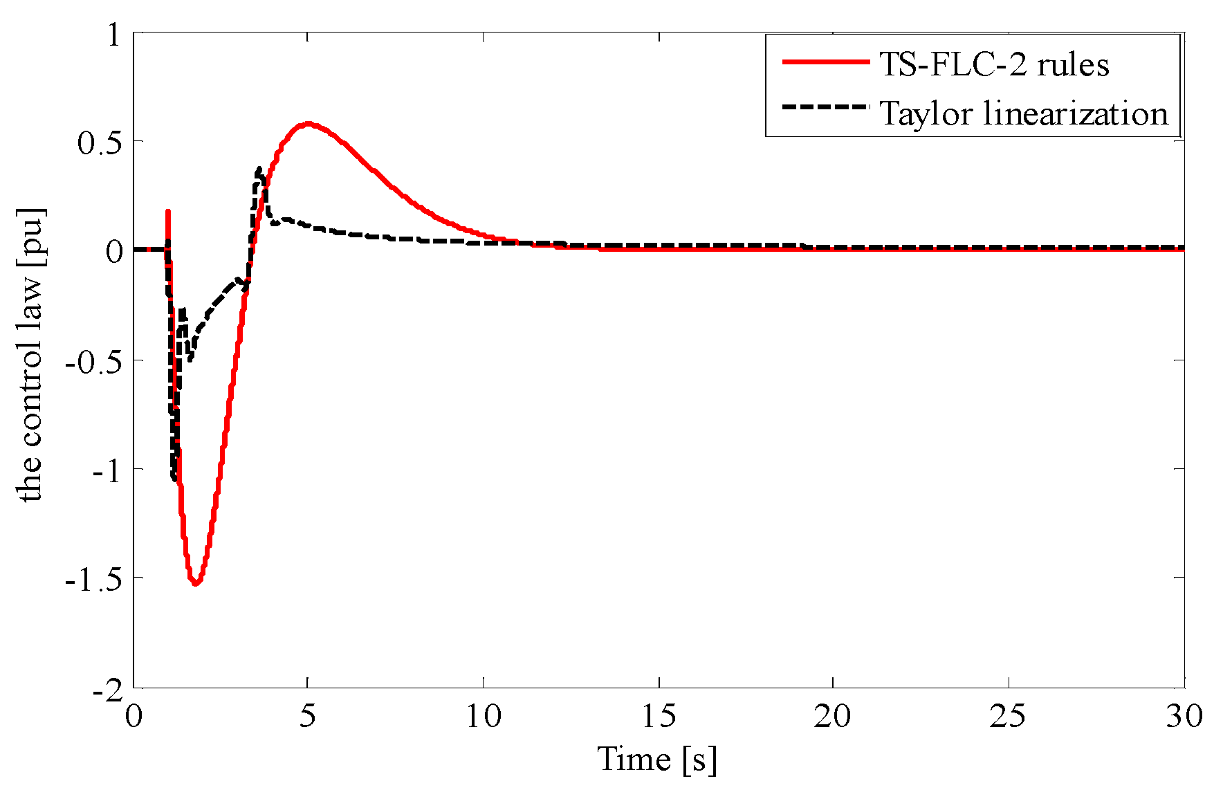
3.2. TS Fuzzy PDC Controller Law

In the PDC design, each control rule is associated with the corresponding two rules of a TS fuzzy model. The obtained values feedback gains Fi for the proposed TS-FLC-2 rules, in the three states, are the following:
  • For the Pre-fault state the control law is:
    U ( t < t 0 ) = i = 1 2 h i ( Z _ ( t ) ) F i X _ ( t ) = ( h 10 1 F p r 1 + h 10 2 F p r 2 ) X _ ( t )
    F p r 1 = [ 10.9398   3.665   18.2035   0.0174   0.0146 0.0067 0.0067   1.0052 ]
    F p r 2 = [ 15.2665   3.3679   18.2106   0.0174   0.0146   0.0067   0.0067   1.0052 ]
  • During fault state the control law is:
    U ( t 0 < t < t e ) = i = 1 2 h i ( Z _ ( t ) ) F i X _ ( t ) = ( h 1 d 1 F d 1 + h 1 d 2 F d 2 ) X _ ( t )
    F d 1 = [ 19.9042   2.4731   19.9329   0.0101   0.0086   0.0031   0.0032   1.0026 ]
    F d 2 = [ 10.7063   2.4736   19.9371   0.0101   0.0086   0.0031 0.0032   1.0026 ]
  • For the Post-fault state the control law is:
    U ( t 0 < t < t e ) = i = 1 2 h i ( Z _ ( t ) ) F i X _ ( t ) = ( h 11 1 F p o 1 + h 11 2 F p o 2 ) X _ ( t )
    F p o 1 = [ 12.7622   3.7120   16.1576   0.0214   0.0166 0.0083 0.0082   1.0061 ]
    F p o 2 = [ 11.0313   3.7109   16.1524   0.0214   0.0166   0.0083   0.0082   1.0061 ]
In addition, for the Taylor linearization method, the feedback gain calculated using LMI in the three states are:
  • Pre-fault state:
    F p r T = [ 0.3513   0.0030   0.7448   0.0032   0.0004   0.0000   0.0000   0.9996 ]
  • During fault state:
    F d T = [ 0.2378   0.0037   0.4380   0.0032   0.0004   0.0000   0.0000   0.9997 ]
  • Post-fault state:
    F p o T = [ 0.2978   0.0035   0.8365   0.0033   0.0003   0.0000   0.0000   0.9997 ]
The application results of the Takagi–Sugeno Fuzzy logic controller TS-FLC-2 rules and Taylor linearization method are shown in Figure 11, Figure 12, Figure 13 and Figure 14.
From the results of the rotor and speed deviations, the reader can figure out that the proposed TS-FLC-2 rules controller is capable to stabilize the power system with an adequate dynamic behavior and satisfactory accuracy and to damp the magnitude within few seconds. However, for Taylor linearization, the simulation time is large and the rotor angle reaches the desired point after 30 s.
Figure 11, Figure 12, Figure 13 and Figure 14 show that the power system reaches and convergences to the desired point. So, the proposed method of rule reduction proves its adequacy to improve the system stability within a transient short time response.
Moreover, relying on the response speed, the disturbance sensitivity, the parameters variation, and the system operating point, it is clear that the robustness and performance are guaranteed. Additionally, according to theorem 1, the system is exponentially globally stable.
Consequently, the advantages of the TS-FLC-2-rule controller can be shown whether at the level of the modeling system or the control system or even the simulation results.
Firstly, for the modeling system, the TS-FLC-2-rule controller decreases the complexity of the system by reducing the linear model number assuming the number of nonlinearities as uncertainties, which facilitates the TS model design and leads to the feasibility of LMI conditions.
Secondly, for the controlling system, the advantages of the proposed approach are the optimization of tuning the fuzzy controller using stability conditions in LMI form and reducing damping.
Finally, for the simulation results, the implementation of the TS-FLC-2-rule controller requires less memory space and computational efforts; it also reduces the simulation time.
The proposed methodology can be experimentally validated by using a prototype composed of a micro-network linked to the computer by using a Digital Communication Card (DSP). Figure 15 presents the general functional block diagram of the real practical application.
To validate this approach, a real-time validation using Hardware-in-the-loop (HIL) simulation can be developed. In fact, the HIL simulation represents the virtual model of the system and the real model of the controller. Then, based on testing, the physical model can be validated.

4. Conclusions

The development of electric power systems has shaped and contributed to the progress in technology over the past century. As a result, the power system has become more and more complex. The model of a power system became nonlinear because of the increase in the number of its components. In addition, it can be affected by disturbances that can cause instability. To cope with this problem, a new TS-FLC method was presented and applied for modeling and controlling power systems even in the presence of disturbances. In spite of the fault perturbation presence, the simulation results proved the performance and effectiveness of the two-rule TS-FLC in controlling, and maintaining stability as well as reducing damping.
In this work, the proposed method was examined under a three-phase short circuit with a short duration. The major advantage of this technique is that it allows good accuracy with a significant gain in computing time. In addition, the proposed controller, considered to control electrical power systems stability based on Takagi–Sugeno (T-S) fuzzy models, can be applicable in the case of a real network in order to enable the network operator to control power system stability at any given disturbance and guarantee service continuity and energy quality to the customer. In this regard, the work presented in this paper serves to quantify and simplify the work of engineers and power system operators.
As continuity to this work and after the practical validation of the proposed approach on Single Machine Infinite Bus (SMIB), this method can be tested on a complicated example (multi-machine network). Then, this concept and design will be discussed in detail on a multi-machine network Western System Coordinating Council (WSCC) comprising three generators and nine nodes.

Author Contributions

Supervision, O.K.; Writing—original draft, R.B.S.; Writing—review & editing, B.A.; Validation, L.K. All authors have read and agreed to the published version of the manuscript.

Funding

This research received no external funding.

Conflicts of Interest

The authors declare no conflict of interest.

Nomenclature

δPower angle of the generator, radian
ωRotor speed of the generator, radian/s
PmMechanical power, p.u
KDDamping constant, p.u
HInertia constant, p.u
Td0Direct axis transient short circuit time constant, s
PeActive electrical power produced by the generator, p.u
EqTransient EMF in the quadratic axis of the generator, p.u
EfdEquivalent EMF in the excitation system, p.u
VtGenerator terminal voltage, p.u
VBInfinite bus voltage, p.u
XTReactance of the transformer, p.u
XLReactance of the transmission line, p.u
XdDirect axis reactance of the generator, p.u
XdDirect axis transient reactance of the generator, p.u
XqQuadratic axis reactance of the generator, p.u
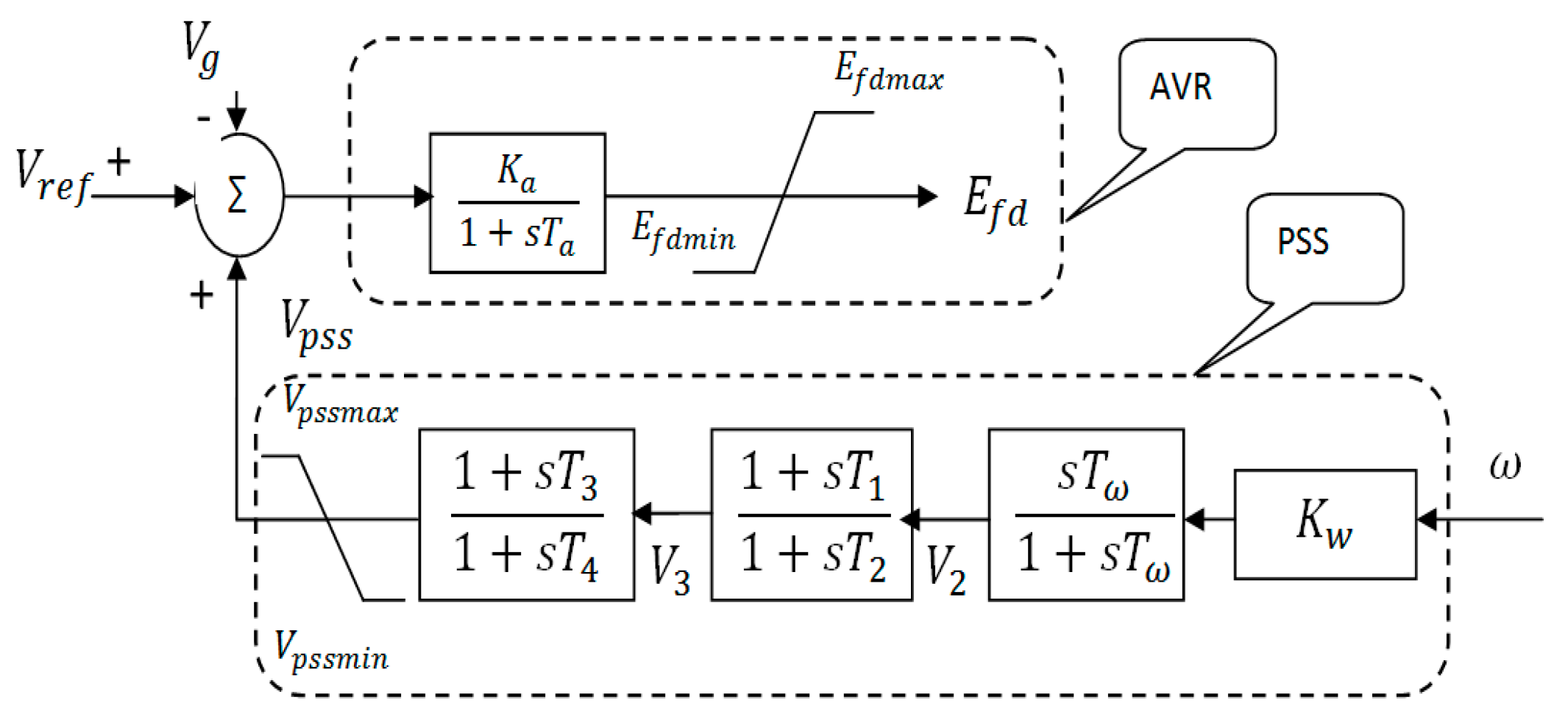
VrefVoltage reference [pu]
VpssPSS output voltage [pu]
TaTime constant of the AVR, s
KaGain of the AVR, p.u.
TωTime constant of the PSS, s
KωGain of the PSS, p.u.
T1, T2Lead-block time constant of PSS, s
T3, T4Lag-block time constant of PSS, s
V1, V2 and V3Intermediate variables of the PSS model

References

  1. Eremia, M.; Shahidehpour, M. Handbook of Electrical Power System Dynamics: Modeling, Stability, and Control; Wiley-IEEE Press: Hoboken, NJ, USA, 2013. [Google Scholar]
  2. Kahouli, O.; Jebali, M.; Alshammari, B.; Abdallah, H.H. PSS design for damping low-frequency oscillations in a multi-machine power system with penetration of renewable power generations. IET Renew. Power Gener. 2019, 13, 116–127. [Google Scholar] [CrossRef]
  3. Gordon, M.; Hill, D.J. Global transient stability and voltage regulation for power systems. In Power and Energy Society General Meeting-Conversion and Delivery of Electrical Energy in the 21st Century; IEEE: Pittsburgh, PA, USA, 2008. [Google Scholar]
  4. Abbadi, A.; Hamidia, F.; Morsli, A.; Tlemcani, A. Optimal voltage controller using t-s fuzzy model for multimachine power systems. Nonlinear Dyn. Syst. Theory 2019, 19, 217–226. [Google Scholar]
  5. Roy, T.K.; Mahmud, M.A.; Shen, W.X. Robust nonlinear adaptive backstepping excitation controller design for rejecting external disturbances in multimachine power systems. Int. J. Electr. Power Energy Syst. 2017, 84, 76–86. [Google Scholar] [CrossRef]
  6. Amoozegar, D. DSTATCOM modelling for voltage stability with fuzzy logic PI current controller. Int. J. Electr. Power Energy Syst. 2016, 76, 129–135. [Google Scholar] [CrossRef]
  7. Yousefian, R.; Kamalasadan, S. A Lyapunov function based optimal hybrid power system controller for improved transient stability. Electr. Power Syst. Res. 2016, 137, 6–15. [Google Scholar] [CrossRef] [Green Version]
  8. Wang, Y.; Zhao, J.; Dimirovski, G.M.; Dimirovski, G.M. Robust adaptive control for a single-machine infinite-bus power system with an SVC. Control Eng. Pract. 2014, 30, 132–139. [Google Scholar] [CrossRef]
  9. Fan, B.; Yang, Q.; Wang, K. Adaptive excitation control of power systems with time-varying constraints. In Proceedings of the 12th World Congress on Intelligent Control and Automation, Guilin, China, 12–15 June 2016. [Google Scholar] [CrossRef]
  10. Kundur, P. Power System Stability and Control; McGraw-Hill: New York, NY, USA, 1994. [Google Scholar]
  11. Salah, R.B.; Djebali, M.; Kahouli, O.; Bouchoucha, C.; Hadj Abdallah, H. Small Signal stability of the tunisian interconnected power system. In Proceedings of the 15th International Conference on Sciences and Techniques of Automatic Control & Computer Engineering, STA’2014, Sousse, Tunisia, 21–23 December 2014. [Google Scholar] [CrossRef]
  12. Salah, R.B.; Kahoul, O.; HadjAbdallah, H. A nonlinear Takagi-Sugeno fuzzy logic control for single machine power system. Int. J. Adv. Manuf. Technol. 2017, 90, 575–590. [Google Scholar] [CrossRef]
  13. Morère, Y. Mise en Œuvre de Lois de Commande Pour les Modèles Flous de Type Takagi-Sugeno. Ph.D. Thesis, Université de Valenciennes et du Hainaut-Cambrésis, Valenciennes, France, 2001. [Google Scholar]
  14. Benzaouia, A.; El Hajjaji, A. Advanced Takagi-Sugeno Fuzzy Systems; Springer: Berlin/Heidelberg, Germany, 2014. [Google Scholar]
  15. Hu, G.; Liu, X.; Wang, L.; Li, H. An extended approach to controller design of continuous-time Takagi–Sugeno fuzzy model. J. Intell. Fuzzy Syst. 2018, 34, 2235–2246. [Google Scholar] [CrossRef]
  16. Tanaka, K.; Wang, H.O. Fuzzy Control Systems Design and Analysis; John Wiley & Sons: Hoboken, NJ, USA, 2001. [Google Scholar]
  17. Zheng, X.; Wang, X.; Yin, Y. Stability analysis and constrained fuzzy tracking control of positive nonlinear systems. Nonlinear Dyn. 2016, 83, 2509–2522. [Google Scholar] [CrossRef]
  18. Yang, F.; Zhang, H.; Wang, Y. An enhanced input-delay approach to sampled-data stabilization of T-S fuzzy systems via mixed convex combination. Nonlinear Dyn. 2014, 75, 501–512. [Google Scholar] [CrossRef]
  19. Chiu, C.H.; Peng, Y.F. Design of takagi-sugeno fuzzy control scheme for real world system control. Sustainability 2019, 11, 3855. [Google Scholar] [CrossRef] [Green Version]
  20. Chang, W.; Wang, W.J. H∞ Fuzzy control synthesis for a large-scale system with a reduced number of LMIs. IEEE Trans. Fuzzy Syst. 2015, 23, 1197–1210. [Google Scholar] [CrossRef]
  21. Ksantini, M.; Ellouze, A.; Delmotte, F. Control of a hydraulic system by means of a fuzzy approach. Int. J. Optim. Control Theor. Appl. 2013, 3, 121–131. [Google Scholar] [CrossRef]
  22. Ghalehnoie, M.; Akbarzadeh-Tootoonchi, M.R.; Pariz, N. Fuzzy control design for nonlinear impulsive switched systems using a nonlinear Takagi-Sugeno fuzzy model. Trans. Inst. Meas. Control 2020, 42, 1700–1711. [Google Scholar] [CrossRef]
  23. Oke, P.; Nguang, S.K. Robust H∞ Takagi–Sugeno fuzzy output-feedback control for differential speed steering vehicles. Proc. Inst. Mech. Eng. Part D J. Automob. Eng. 2020, 234, 2822–2835. [Google Scholar] [CrossRef]
  24. Sung, H.C.; Park, J.B. Robust fuzzy control for a hybrid magnetic bearings: The relaxed stabilization condition approach. Nonlinear Dyn. 2016, 85, 2487–2496. [Google Scholar] [CrossRef]
  25. José, V. T–S Fuzzy bibo stabilisation of non-linear systems under persistent perturbations using fuzzy lyapunov functions and non-pdc control laws. Int. J. Appl. Math. Comput. Sci. 2020, 30, 529–550. [Google Scholar]
  26. Tanaka, K.; Tanaka, M.; Chen, Y.J.; Wang, H.O. A new sum- of- squares design framework for robust control of polynomial fuzzy system with uncertainties. IEEE Trans. Fuzzy Syst. 2016, 24, 94–110. [Google Scholar] [CrossRef]
  27. Nguyen, A.T.; Taniguchi, T.; Eciolaza, L.; Campos, V.; Palhares, R.; Sugeno, M. Fuzzy control systems: Past, present and future. IEEE Comput. Intell. Mag. 2019, 14, 56–68. [Google Scholar] [CrossRef]
Figure 1. Single machine power system.
Symmetry 12 02068 g001
Figure 2. Automatic Voltage Regulator (AVR) and Power System Stabilizer (PSS) controllers.
Symmetry 12 02068 g002
Figure 3. Fuzzy controller design-based model.
Symmetry 12 02068 g003
Figure 4. Simulink Model of the studied power system.
Symmetry 12 02068 g004
Figure 5. Rotor angle responses.
Symmetry 12 02068 g005
Figure 6. Speed deviation responses.
Symmetry 12 02068 g006
Figure 7. Transient voltage deviations.
Symmetry 12 02068 g007
Figure 8. Excitation voltage variation.
Symmetry 12 02068 g008
Figure 9. PSS output voltage.
Symmetry 12 02068 g009
Figure 10. Controllaw variation.
Symmetry 12 02068 g010
Figure 11. Rotor angle responses.
Symmetry 12 02068 g011
Figure 12. Speeddeviation responses.
Symmetry 12 02068 g012
Figure 13. Transient voltage response.
Symmetry 12 02068 g013
Figure 14. Control law variation.
Symmetry 12 02068 g014
Figure 15. Generalfunctional block diagram of the real practical application.
Symmetry 12 02068 g015
Table 1. System parameters.
VariablesValuesVariablesValues
Pe0.9XL20.93
Qe0.436XT0.15
Vt1Ka250
f50Ta0.015
Xd1.81T10.9471
Xq1.494T21.0175
X′d0.3T30.6725
Xq0.65T40.6756
Td08Kw45.8373
H3.5Tw1.0871
D0.01TE1
XL10.5
Table 2. System state.
VariablesValues
δ 0 1.178
w 0 0
E q 0 1.0474
E f d 0 2.4160
V 10 , V 20 , V 30 , V p s s 0 0
δ d 1.368
ω d 0
E q d 1.0474
E f d d 2.4160
V 1 d , V 2 d , V 3 d , V p s s d 0
Publisher’s Note: MDPI stays neutral with regard to jurisdictional claims in published maps and institutional affiliations.

