Investigation of Position and Velocity Stability of the Nanometer Resolution Linear Motor Stage with Air Bearings by Shaping of Controller Transfer Function

Abstract

Modern industrial enterprises require high accuracy and precision feedback systems to fulfil cutting edge requirements of technological processes. As demand for a highly accurate system grows, a thin gap between throughput and quality exists. The conjunction of ultrafast lasers and modern control strategies of mechatronic systems can be taken into account as an effective solution to reach both throughput and tolerances. In the present paper, the dynamic errors of the moving platform of the one degree of freedom stage, based on linear motor and air bearings, have been analyzed. A precision positioning system is investigated as a symmetric system which is based on symmetric linear motor. The goal of the present article is to investigate the controllers of the different architecture and to find the best controller that can ensure a stable and small dynamic error of the displacement of the stage platform at four different constant velocities of the moving platform. The relations between the controller order, velocity and the displacement dynamic error have been investigated. It is determined that higher-order controllers can reduce the dynamic error significantly at low velocities of the moving platforms: 1 and 5 mm/s. On the contrary, the low order controllers of 4th-degree polynomials of the transfer function can also provide small dynamic errors of the displacement of the platform.

1. Introduction

High-resolution systems with the lowest possible velocity are important for both industry and fundamental physics research. On the one hand, there is the requirement to ensure the low velocity in the interferometric application, which is used to research fundamental physical relationships; on the other hand, it is important to maintain as stable as possible micrometer level velocity in the technological process to ensure the minimal possible influence of dynamic error and mechanical “jitter.” In most cases, the performance of linear motor stages is investigated in high velocity regimes, but there is a lack of research that is related to the stability of a relatively low velocity linear motor and air bearing system. The velocity loop in a cascade control system and a velocity feedback source play a significant role in settling process of sensitive positioning systems, its damping control and stability [1,2].

High-performance industrial processes are often automated by applying positioning systems that are based on linear motor and air bearings. Positioning systems which are based on linear motors and air bearings do not have gears and ball or rollers in their guides. Therefore, after their calibration and tuning (stabilization), the systems do not require maintenance because of geometry degradation or loosening of greases. Air bearing and linear motor-based systems are widely integrated to machines where high velocity, high machine accuracy and precision are important [3,4,5,6]. Usually, air bearing is sliding on a thin air film; therefore, no friction is applied, which means no maintenance and degradation will occur. The accuracy of the machines based on the air bearings is strongly dependent on the surface quality (especially flatness) in air bearing operating zones. Depending on the environment condition and stage design, air bearings might be operated with different kinds of gases instead of compressed air. On the other hand, in air bearing systems, there is no damping, which is usually observed in stages of the mechanical guiding system. Therefore, air bearing systems are very sensitive and aggressively tuned. These systems can even suddenly become unstable because of noise coming from the motor amplifier. To stabilize the air bearing stages, it is required to precisely fit the controller transfer function and necessary filters (or, for example, use a Kalman filter) and control it by using the sliding control mode (SCM). Therefore, it is required to estimate the damping which occurs because of Eddy Current (ECD) [7,8,9]. To add a Kalman filter or SMC to the control system, special system diagnostics must be undertaken, including frequency response function (FRF) identification, control loop shaping and its fitting to required conditions [10,11,12].

Direct drive mechanisms are mandatory if there are requirements to minimize the static and dynamic errors of the displacement [13,14,15,16,17]. In the majority of cases with mechanical guiding system-based long travel linear motor stage with air bearings (LMS), these errors are caused by various imperfections such as backlash, a lack of precision for component assembly, preload, eigenfrequencies of parts, errors of the measurement system, altering or even nonoperational ambient conditions, etc. In case of air bearing LMS, the abovementioned factors might be reduced to a damping factor. Linear motors are “direct drive” systems where no gears (such as a ball screw, belt drive, rack and pinion) are required to transform a rotary motion to a linear motion. Linear force is generated by a “Lorentz force,” induced proportionally to the added current: $\left(\overrightarrow{F}=I\overrightarrow{L}x\overrightarrow{B}\right)$. Linear motor systems with air bearings can be analyzed as a linear dynamic system. However, to be precise, there may be dampings that should be taken into account if sub micrometer or nanometer precision has to be reached out.

The displacement errors of the positioning systems are still under intensive investigations since, on the one hand, it is important to ensure the required precision for a long term of the operating of the positioning systems; on the other hand, it is very important to have a diagnostic methodology to warrant the required precision. These requirements actualize many factors that can affect the errors: the materials, the design of the system, the control approach, the motion mode (for example velocity) and so on. For example, the influence of the porosity to the piezo effect of the symmetric piezo ceramic beam was investigated in [18], while the design factors affecting the preciseness of the displacement were discussed in [19]. In this paper, it is concluded that the main factor affecting the error is the micrometer gap (backlash) between. However, in this article, there is no information related to the frequency mode that leads to the degradation of the gear. The investigation of the flexible rotor with the air bearings and its dynamic behavior is presented in [20]. The forward kinematics and dynamics of the mechanical systems of the multi-degree of freedom connected in series was investigated in [21].

It should also be noticed that the stability and bandwidth of systems may depend on the human factor, which affects the assembly and mechanical adjustment of the system. The errors entailed by the human factor are not systematic, and therefore, are difficult to predict without interrupting the highly qualified engineering staff [22]. It should be noted that the analysis of the systems with air bearings and linear motors is only a control engineering problem, since these systems have no mechanical stiffness and damping.

In the particular investigation, iron-less motor-based positioning system of the symmetrical design was investigated. The linear force generated by the stage is guaranteed by the motor windings that are symmetrically placed in the mover of the motor. The mover is placed to the symmetric “U-Shape” permanent magnet tack based on the classic “Halbach” array. The force of the motor and it inducing current is characterized by the motors’ force constant that strongly depends on the magnet type, its internal design and symmetry of the windings. The moving part is placed on symmetrically distributed air-bearings.

The main aim of the present investigation is to understand the possibility to ensure position and velocity stability of the stage platform by identifying the transfer function of the plant and by applying the proportional-integral-derivative controllers, denoted hereafter as PID, with different filters. In the present article, PID with the low pass filter is denoted hereafter by PID1; PID with the low pass and notch filters is denoted by PID2; and PID with the low pass, notch and bi-quad filters is denoted by PID3. The investigation results should be useful to ensure the stability of the system under investigation with minimum arrangements. That is, without any additional efforts to modify the plant mechanically or to change the plant itself. The setup is based on a granite base, air bearing, three-phase brushless DC motor made by “Tecnotion UM9N,” which is controlled by position and velocity control regulator “ACS Motion Control UDMsd.” The control loops are closed by the Michelson laser interferometer “Renishaw XL-80” with 24-bit output that is converted to the industrial digital differential quadrature RS-422 signal output. Particular architecture of the stage is quite popular in ultra-high precision industrial architecture; therefore, the investigation might help in the control and preparation of similar systems.

To identify the plant, it is excited by the frequency-based sinusoidal current (or force) of the constant amplitude, while the system is commanded to move at a constant speed. The procedure of the identification performed during the motion of the plant allows us to estimate the transfer function of the plant and open loop system without the influence of the static damping effects caused by cables, drag chain and so on. An additional tool to identify the transfer functions is the accelerometer. Accelerometers play an important role in experiments, since they allow us to compare identified eigenfrequencies to the harmonic excitation obtained by the FRF of the plant.

The obtained results of the investigation are represented by the derived transfer functions of the plant, controllers and the whole open loop LMS. The experimentally identified frequency response functions (FRF) are compared with the FRF of the theoretically derived transfer functions of the LMS.

2. Materials and Methods

The object of investigation. The one degree of freedom-long travel linear motor stage with air bearings, hereafter denoted as LMS, see Figure 1, consists of: a moving platform (pos 1 of Figure 1), a granite base (pos. 2 of Figure 1), accelerometers (pos. 3 of Figure 1), load (pos. 4 of Figure 1), an interferometer mirror (pos. 5 of Figure 1), air bearings (pos. 6 of Figure 1) and a three-phase ironless linear brushless DC motor (pos. 7 of Figure 1).

LMS is assembled on a heavy granite base (pos. 2 of Figure 1) along with the load (pos. 4 of Figure 1) to ensure stability. Position and velocity control loops of the platform are both closed by a Michelson laser interferometer. The mirror (pos. 5 of Figure 1) of the interferometric measurement system is attached directly to the moving platform (pos. 1 of Figure 1) to ensure the precise displacement feedback. In the LMS under consideration, the guiding system is the air bearings system (pos. 6 of Figure 1). Bandwidth and partially frequency response of the LMS is estimated by accelerometers (pos. 3 of Figure 1).

The test equipment. The test stand consists of: a granite base (pos. 1 of Figure 2), a Michelson laser interferometer (pos. 2 of Figure 2), LMS (pos. 3 of Figure 2), a PC with control and diagnostic software (pos. 4 of Figure 2) and a motion controller and amplifier module (pos. 5 of Figure 2). The general view of the test equipment is shown in Figure 2.

Motor windings are directly connected to current amplifier UDMSD2B2N0N, which is part of the motion control setup (pos. 5 of Figure 2). Position and velocity control loops of the platform are both closed by a Michelson laser interferometer RENISHAW XL-80 (pos. 2 of Figure 2). As a result, the interferometer (pos. 2 of Figure 2) provides the quantized output, which is based on the digital differential RS-422 interface. The RS-422 interface output of the digital interferometer (pos. 2 of Figure 2) is directly connected to the current amplifier UDMSD2B2N0N, which is part of the motion control setup (pos. 5 of Figure 2). The motion controller (single board computer or master) SP with EC-04000032NAN5NDNN is used to establish the communication with a PC (pos. 4 of Figure 2) using TCP/IP interface from one side, and UDMSD2B2N0N (or slave) using EtherCAT interface from the other side. Furthermore, by using a PC (pos. 4 of Figure 2) and a combination based on motion controller SP with EC-04000032NAN5NDNN and current amplifier UDMSD2B2N0N (pos. 5 of Figure 2), real time control and diagnostics of LMS (pos. 3 of Figure 2) will be investigated. To obtain the frequency response functions of LMS, it is excited by the current of the limited bandwidth and amplitude (which might be considered as force excitation). The bandwidth is compared with the results obtained by the accelerometers.

In the next stage, the controllers PID1, PID2 and PID3 are examined by comparing the displacement dynamic errors of the platform of LMS with different PIDs. Additionally, the Fourier spectral analysis of the amplitudes of the displacement dynamic errors is performed.

Mathematical modelling of the long travel linear motor stage with air bearings. The block diagram of LMS and control system is shown in Figure 3. LMS with a current amplifier (including current control loop which consists of “proportional-integral” controller) is hereafter called the plant, see Figure 3. After tuning of the current loop, the plant is considered as a constant, while the influence of the different velocity loop shaping filters, LPF (second order low pass filter), NF (second order notch filter) and BF (second order bi-quad filter), is investigated. As was already mentioned, in the present article, the position and velocity loops together with the velocity loop shaping filters are called controller PID1, when LPF is applied; controller PID2, when LPF and NF are applied; and controller PID3 when LPF, NF and BF are applied.

The position and velocity loops together comprise the control system. The position loop corresponds to the “proportional” controller, a velocity loop which consists of the “proportional-integral” controller and “loop shaping filters.” Furthermore, the influence on the dynamic error of certain filter combination will be investigated.

The mathematical modelling of LMS is based on the following assumptions:

(1)

No friction forces appear in the moving LMS parts;

(2)

All parts of the LMS are absolutely rigid. That is, only the rigid body dynamics is considered in the present investigation;

(3)

There is no backlash in the connections of the moving LMS parts;

(4)

The motion of the all moving LMS parts is straight-linear;

(5)

The displacements of all the moving LMS parts are identical;

(6)

The current amplifier is considered as linear after tuning of the PI controller in the current control loop;

(7)

The moving mass is constant and the amplifier bus voltage is constant;

(8)

The environmental conditions are constant and well-controlled.

3. Modeling and Identification

3.1. Governing Equations

In the present section, the transfer functions of the open loop system consisting of the plant and the controller are derived analytically. To assess the accuracy of the analytically obtained transfer functions, the frequency response functions obtained from the transfer functions were compared with the experimentally identified frequency response functions of the open loop systems of LMS consisting of different controllers: PID1, PID2 and PID3.

The system of the governing differential equations of the LMS consists of three equations that relate the displacement of the LMS platform, the electromechanical parameters of the LMS devices and the current and voltage:

$$m_{tot}\frac{d^{2}x\left(t\right)}{d{t}^2}=F_{motor}\left(t\right)$$

(1)

$$F_{motor}\left(t\right)=K_{t}I\left(t\right)$$

(2)

$$L\frac{dI\left(t\right)}{dt}+RI\left(t\right)=U-K_e\frac{dx\left(t\right)}{dt}$$

(3)

From Equations (1)–(3), it follows that:

$$L\frac{dI\left(t\right)}{dt}+R\frac{m_{tot}}{K_t}\frac{d^{2}x\left(t\right)}{d{t}^2}=U-K_e\frac{dx\left(t\right)}{dt}$$

(4)

where $t$ is time (s); $x$ is displacement of the LMS platform, see Figure 1, (m); $\dot{x}$ (m/s) and $\ddot{x}$ ($\mathrm{m}/{\mathrm{s}}^{-2}$) are the velocity and acceleration of the LMS platform or the first and the second order time derivatives of the displacement $x$ of the LMS platform, respectively; $m_{tot}=100$ (kg) is the total mass of the parts of the LMS platform that move in the straight-line motion; $I$ is the current (A); $F_{motor}$ is the motor generated force (N); $K_t=36.3$ (N/A) is the motor force constant; $L=2.0$ (mH) is the inductance of the motor winding; $R=6.2$ (Ohm) is the resistance of the motor winding; U = 48 (VDC) is the nominal bus voltage; and $K_e=30.0$ ($\left(\mathrm{V}\mathrm{s}\right)/\mathrm{m}$) is the motor Back EMF constant. In Equations (1)–(3), the current I is a time-dependent given function, while quantities $m_{tot}$, $K_t$, $K_e$, $L$, $R$ and $U$ are time-independent constant parameters. The displacement $x\left(t\right)$, velocity $dx\left(t\right)/dt\stackrel{\mathrm{def}}{=}\dot{x}\left(t\right)$ and acceleration $d^{2}x\left(t\right)/d{t}^2\stackrel{\mathrm{def}}{=}a\left(t\right)$ of the LMS platform are unknown time functions.

As illustrated in Figure 3, the plant consists of: motor, air bearing, current amplifier and current controller, which is considered linear after the current loop is tuned. The current controller might be represented as the transfer function given in Equation (5), which represents the PID controller:

$$i\left(s\right)=K_p+\frac{K_i}{s}+K_d\cdot s=\frac{K_P\cdot s+K_i+K_d\cdot s^2}{s}$$

(5)

where $K_p=570$ is proportional coefficient of PID controller; $K_i=6000$ is integral coefficient of PID controller; $K_d=0$.

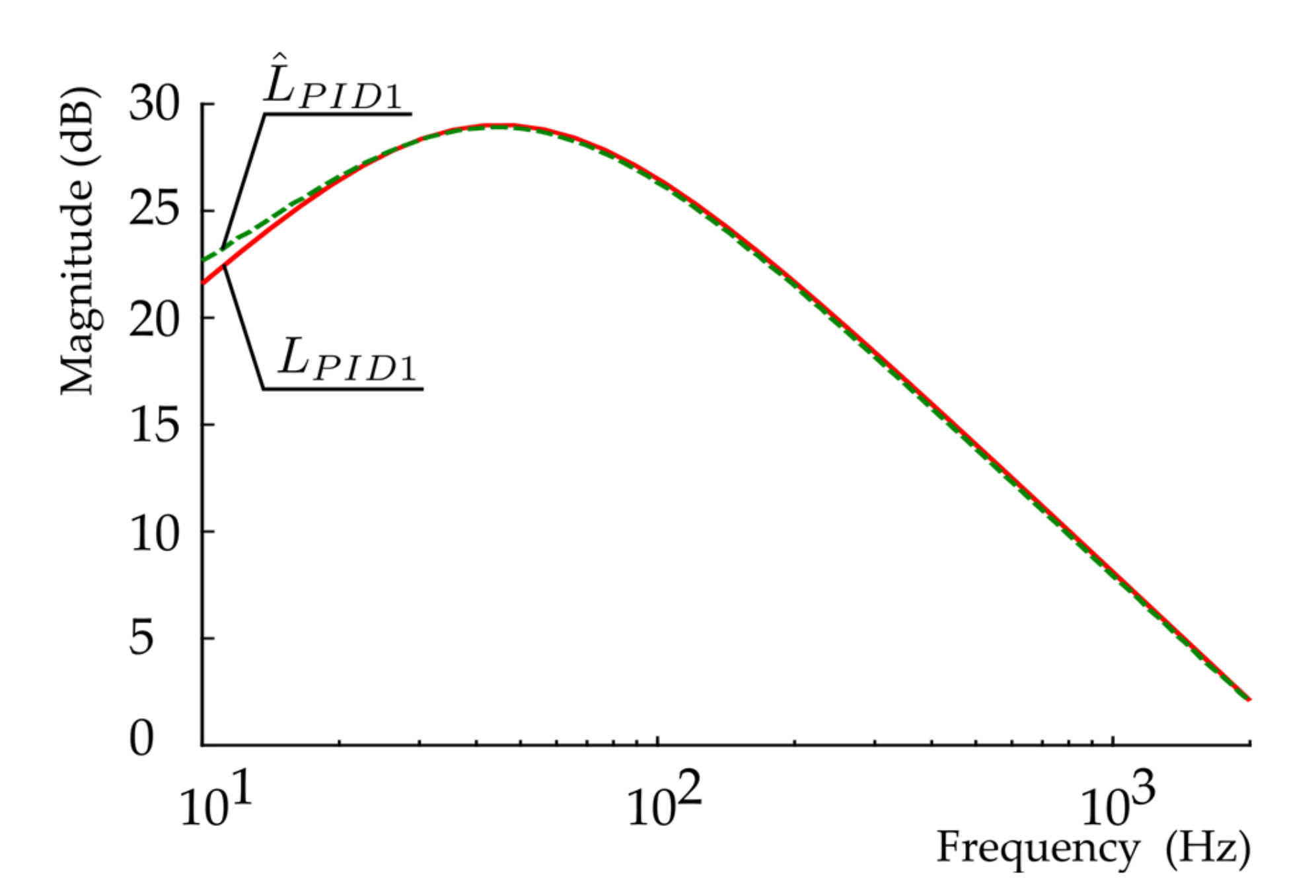
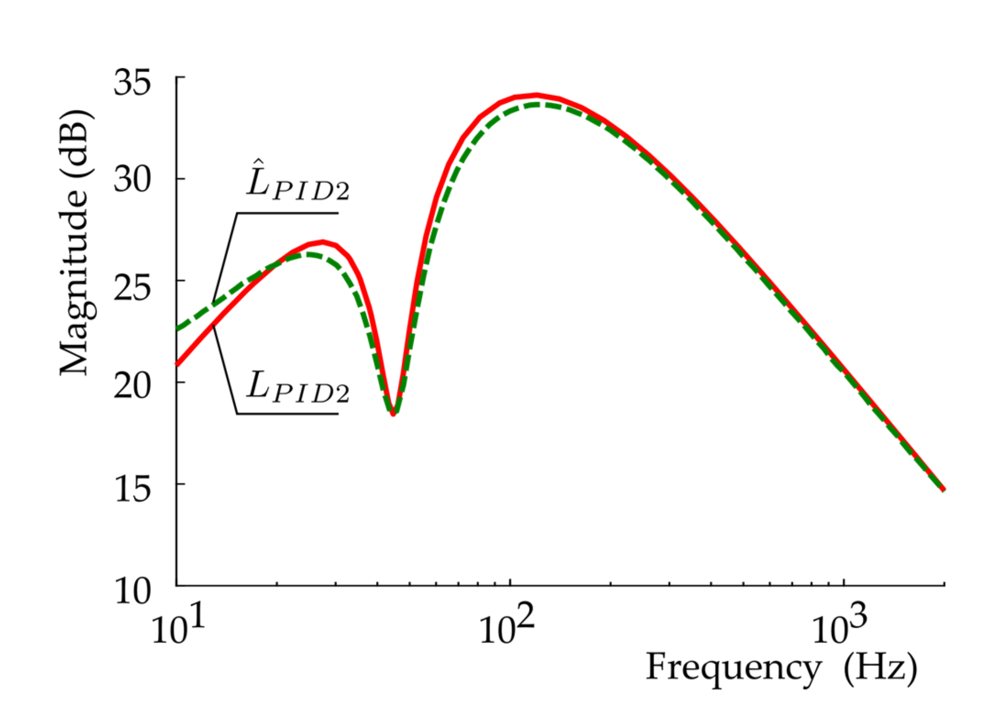
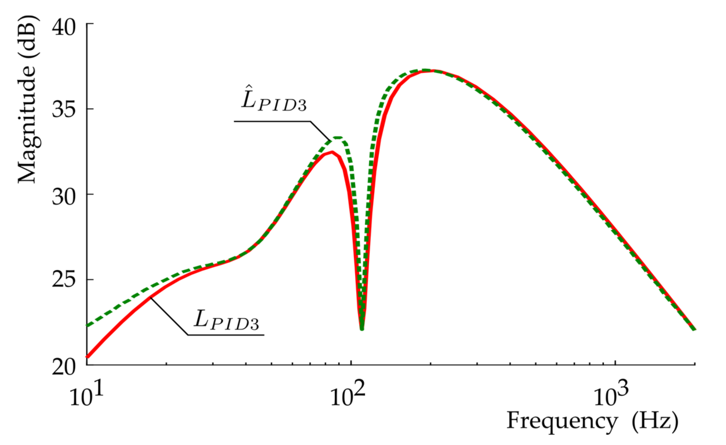
3.2. Theoretical Transfer Functions, Their Frequency Response Functions and a Comparison with the Experimentally Identified Frequency Response Functions

The transfer functions obtained in this section will be written as ratios of polynomials and will be illustrated graphically and compared with the experimental results. Factorized style transfer function expressions will not be presented here in order to have more compact equations, to simplify the modelling by mathematical software tools. The structure of the controller is presented in Figure 3, while PID coefficients and filter bandwidths are represented in

Table 1. Summarized parameters of the transfer functions $H_{PID1}$, $H_{PID2}$ and $H_{PID3}$.

Parameter	${\mathit{H}}_{\mathit{P}\mathit{I}\mathit{D}1}$	${\mathit{H}}_{\mathit{P}\mathit{I}\mathit{D}2}$	${\mathit{H}}_{\mathit{P}\mathit{I}\mathit{D}3}$
LPF cut off frequency, Hz	45	98	150
NF central frequency, Hz	-	45	110
BF central frequency, Hz	-	-	45
BF type	-	-	Notch filter
Position loop P coefficient	5	5	5
Velocity loop P coefficient	200	180	180
Velocity loop I coefficient	120	160	160

. The transfer function of the plant, denoted by $H_{PLANT}$, which includes the motor current amplifier, see Equation (4), and the current controller, see Equation (5), in the frequency domain, can be represented as the following polynomial ratio:

$$H_{PLANT}\left(s\right)=\frac{2.586\cdot {10}^7\cdot s+2.722\cdot {10}^8}{2\cdot {10}^{-1}\cdot s^4+5.762\cdot {10}^4\cdot s^3+6\cdot {10}^5\cdot s^2}$$

(6)

Before starting the analysis of the dynamic errors of LMS, the experimental identification of PLANT was conducted by defining the empirical FRFs ${\widehat{L}}_{PLANT1}$, ${\widehat{L}}_{PLANT2}$ and ${\widehat{L}}_{PLANT3}$. Additionally, these functions ${\widehat{L}}_{PLANTi}$, $i\in \left\{1,2,3\right\}$ were compared with the FRF of the theoretical transfer function $H_{PLANT}$, denoted by $L_{PLANT}$. These frequency response functions are depicted in Figure 4.

From Figure 4, we can observe that the experimentally determined behavior of the real PLANT remains constant for all investigated controller cases and has a set of the eigenfrequencies that can have an influence on the whole stability, settling time and settling window of LMS. As is mentioned above, LMS is frictionless and based on the air bearings. Therefore, eigenfrequencies can be caused by the structure of LMS, cable management etc. The more detailed mechanical analysis and design revisions can be considered to damp the parasitic resonances of the system. However, in the present investigation, the influence of the architecture of the velocity control loop has been taken into account and investigated to understand if the eigenfrequencies can be damped by using the only loop shaping filters.

In the first case, a relatively simple (standard/straightforward) architecture of the controller PID1 was investigated. PID1 is made of the control system, see Figure 3, by adding the second-order low pass filter to the velocity loop to shape the velocity loop and damp the low-frequency resonances. Cut off frequency of the added LPF is 45 Hz. The analytically derived theoretical transfer function of PID1 in the frequency domain can be written as follows:

$$H_{PID1}=\frac{2\cdot {10}^2\cdot s^3+1.12\cdot {10}^3\cdot s^2+6\cdot {10}^2\cdot s}{1.25\cdot {10}^{-2}\cdot s^4+7.074\cdot s^3+1\cdot {10}^3\cdot s^2}$$

(7)

The experimental identification of the FRF of PID1, denoted hereafter as ${\widehat{L}}_{PID1}$, was also conducted. The experimental and theoretical FRFs ${\widehat{L}}_{PID1}$ and $L_{PID1}$, where $L_{PID1}$ is the FRF of $H_{PID1}$, given in Equation (7), are depicted in Figure 5.

Controller PID2 has been investigated in the second case. LPF and the second-order notch filter (NF) are added in the velocity loop of PID2. NF is added to damp the particular narrow bandwidth in the frequency domain. The cut-off frequency of the newly added LPF is 98 Hz, while NF is wrapped around a 45 Hz frequency.

The transfer function of controller PID2, denoted by $H_{PID2}$, in the frequency domain can be written as follows:

$$H_{PID2}\left(s\right)=\frac{1.8\cdot {10}^2\cdot s^5+1.006\cdot {10}^4\cdot s^4+1.444\cdot {10}^7\cdot s^3+8.478\cdot {10}^7\cdot s^2+6.396\cdot {10}^7\cdot s}{2.637\cdot {10}^{-3}\cdot s^6+3.911\cdot s^5+2.027\cdot {10}^3\cdot s^4+5.11\cdot {10}^5\cdot s^3+7.994\cdot {10}^7\cdot s^2}$$

(8)

The experimental identification of the FRF of PID2, denoted by ${\widehat{L}}_{PID2}$, has also been conducted. The theoretical FRF $L_{PID2}$ of $H_{PID2}$, see Equation (8), and the experimental FRF ${\widehat{L}}_{PID2}$ are shown in Figure 6.

Controller PID3 has been investigated in the third case. Three filters have been added to the velocity loop of PID3. In addition to LPF and NF, added in PID2, the extra second-order bi-quad filter (BF) has been added to the velocity loop to damp the second particular narrow bandwidth in the frequency domain. It should be noted that it is impossible to continuously increase an order of the velocity loop because of the decreasing phase margin. The cut-off frequency of the newly added LPF is 150 Hz, the NF is wrapped around 110 Hz frequency and the second-order BF that is designed as an NF is wrapped around 45 Hz. In the present third case, the transfer function of controller PID3, denoted by $H_{PID3}$, in the frequency domain can be written as follows:

$$H_{PID3}=\left({{\displaystyle \sum }}_{i=1}^7{a}_i{s}^i\right){\left({{\displaystyle \sum }}_{i=2}^8{b}_j{s}^j\right)}^{-1}$$

(9)

where coefficients $a_i$ and $b_j$ are the following: $a_1=3.822\cdot {10}^8$, $a_2=5.077\cdot {10}^8$, $a_3=8.783\cdot {10}^7$, $a_4=3.207\cdot {10}^5$, $a_5=1.292\cdot {10}^3$, $a_6=7.625\cdot {10}^{-1}$, $a_7=2.252\cdot {10}^{-3}$, $b_2=4.777\cdot {10}^8$, $b_3=4.644\cdot {10}^6$, $b_4=1.699\cdot {10}^4$, $b_5=3.288\cdot {10}^1$, $b_6=4.404\cdot {10}^{-2}$, $b_7=3.805\cdot {10}^{-5}$, $b_8=1.408\cdot {10}^{-8}$.

As in the previous cases of the controllers PID1 and PID2, the experimental identification of the FRF of PID3, denoted by ${\widehat{L}}_{PID3}$, has also been conducted. The theoretical and experimental frequency response functions $L_{PID3}$ of $H_{PID3}$, see Equation (9), and ${\widehat{L}}_{PID3}$ are depicted in Figure 7.

The scheme of the controller is shown in Figure 3. In case of the velocity loop architecture, loop shaping filters are connected in series. The parameters of the transfer functions $H_{PID1}$, $H_{PID2}$ and $H_{PID3}$ of the corresponding controllers are summarised in Table 1.

Generalization of transfer functions $H_{PLANT}$, see Equation (6), and $H_{PID1}$, see Equation (7), yields the transfer function of the open loop system consisting of the controller and the plant (in the frequency domain):

$$H_{OLSYS1}\left(s\right)=\frac{5.173\cdot {10}^9\cdot s^4+8.342\cdot {10}^{10}\cdot s^3+3.204\cdot {10}^{11}\cdot s^2+1.634\cdot {10}^{11}\cdot s}{2.502\cdot {10}^{-3}\cdot s^8+7.222\cdot {10}^2\cdot s^7+4.153\cdot {10}^5\cdot s^6+6.186\cdot {10}^7\cdot s^5+6.000\cdot {10}^8\cdot s^4}$$

(10)

The experimental identification of the FRF of the open loop system (denoted hereafter by ${\widehat{L}}_{OLSYS1}$) was conducted to assess the accuracy of the theoretically obtained transfer function $H_{OLSYS1}$, see Equation (10), of the open loop of the system. The experimentally and analytically obtained FRFs ${\widehat{L}}_{OLSYS1}$ and $L_{OLSYS1}$ are depicted in Figure 8. I should be noted that in this particular case, the bandwidth of LMS is 13.6 Hz, the gain margin is 5.8 dB and the phase margin is 29.

Generalization of the transfer functions $H_{PLANT}$, see Equation (6), and $H_{PID2}$, see Equation (8), yields the transfer function of the open loop system consisting of the controller (LPF and NF) and PLANT (in frequency domain):

$$H_{OLSYS2}=\left({{\displaystyle \sum }}_{i=1}^6{a}_i{s}^i\right){\left({{\displaystyle \sum }}_{i=4}^{10}{b}_j{s}^j\right)}^{-1}$$

(11)

where coefficients $a_i$ and $b_j$ are the following: $a_1=1.741\cdot {10}^{16}$, $a_2=2.474\cdot {10}^{16}$, $a_3=6.125\cdot {10}^{15}$, $a_4=3.763\cdot {10}^{14}$, $a_5=3.092\cdot {10}^{11}$, $a_6=4.655\cdot {10}^9$, $b_4=4.797\cdot {10}^{13}$, $b_5=4.913\cdot {10}^{12}$, $b_6=3.068\cdot {10}^{10}$, $b_7=1.193\cdot {10}^8$, $b_8=2.273\cdot {10}^5$, $b_9=1.528\cdot {10}^2$, $b_{10}=5.275\cdot {10}^{-4}$.

As in the previous case, the FRF of the open loop system was identified experimentally, denoted by ${\widehat{L}}_{OLSYS2}$, and compared with the FRF of the theoretical transfer function $H_{OLSYS2}$, see Equation (11). The graphs of FRFs ${\widehat{L}}_{OLSYS2}$ and $L_{OLSYS2}$ are shown in Figure 9. The bandwidth of this LMS is 13.6 Hz, the gain margin is 5.7 dB and the phase margin is 29.

Finally, the theoretical transfer functions $H_{OLSYS3}$, see Equation (12), defined over the frequency domain, of the open loop system of LMS was obtained by combining the transfer functions $H_{PLANT}$, see Equation (6), and $H_{PID3}$, see Equation (9):

$$H_{OLSYS3}=\left({{\displaystyle \sum }}_{i=1}^8{a}_i{s}^i\right){\left({{\displaystyle \sum }}_{i=4}^{12}{b}_j{s}^j\right)}^{-1}$$

(12)

where coefficients $a_i$ and $b_j$ are the following: $a_1=1.040\cdot {10}^{17}$, $a_2=1.481\cdot {10}^{17}$, $a_3=3.704\cdot {10}^{16}$, $a_4=2.359\cdot {10}^{15}$, $a_5=8.646\cdot {10}^{12}$, $a_6=3.362\cdot {10}^{10}$, $a_7=2.033\cdot {10}^7$, $a_8=5.823\cdot {10}^4$, $b_4=2.866\cdot {10}^{14}$, $b_5=3.031\cdot {10}^{13}$, $b_6=2.779\cdot {10}^{11}$, $b_7=9.999\cdot {10}^7$, $b_8=1.924\cdot {10}^6$, $b_9=2.567\cdot {10}^3$, $b_{10}=2.21$, $b_{11}=8.190\cdot {10}^{-4}$, $b_{12}=2.816\cdot {10}^{-9}$. The empirical FRF of the open loop of LMS, denoted by ${\widehat{L}}_{OLSYS3}$, was experimentally identified and depicted together with the FRF, denoted by $L_{OLSYS3}$, of the transfer function $H_{OLSYS3}$ for the purpose of the comparison (see Figure 10). For this third case, the bandwidth of LMS is 12.7 Hz, the gain margin is 5.6 dB and the phase margin is 29.

From Figure 8, Figure 9 and Figure 10, we can conclude that the analytically obtained transfer functions $H_{OLSYSi}$, $i\in \left\{1,2,3\right\}$, given in Equations (10)–(12), respectively, of the open loop systems of LMS with different controllers, PID1, PID2 and PID3, are accurate enough, and the stability of these LMS are also good enough in the frequency domain.

4. Results and Discussion

In the present section the quasi stable LMSs in the time domain are investigated. These LMSs, with different controllers PID1, PID2, PID3, were examined by measuring the dynamic error of the displacement of the stage platform, see detail 1 in Figure 1. The displacements were entailed by exciting LMSs with different velocities {1, 5, 10, 20} mm/s; the mass of the moving platform and the acceleration and jerk were constant.

Three configurations of the controller were analyzed: PID1 (where only LPF is used), PID2 (where LPF and NF are used) and PID3 (where LPF, NF and BF are used). In each phase of the experiment, the following activities were arranged:

(1)

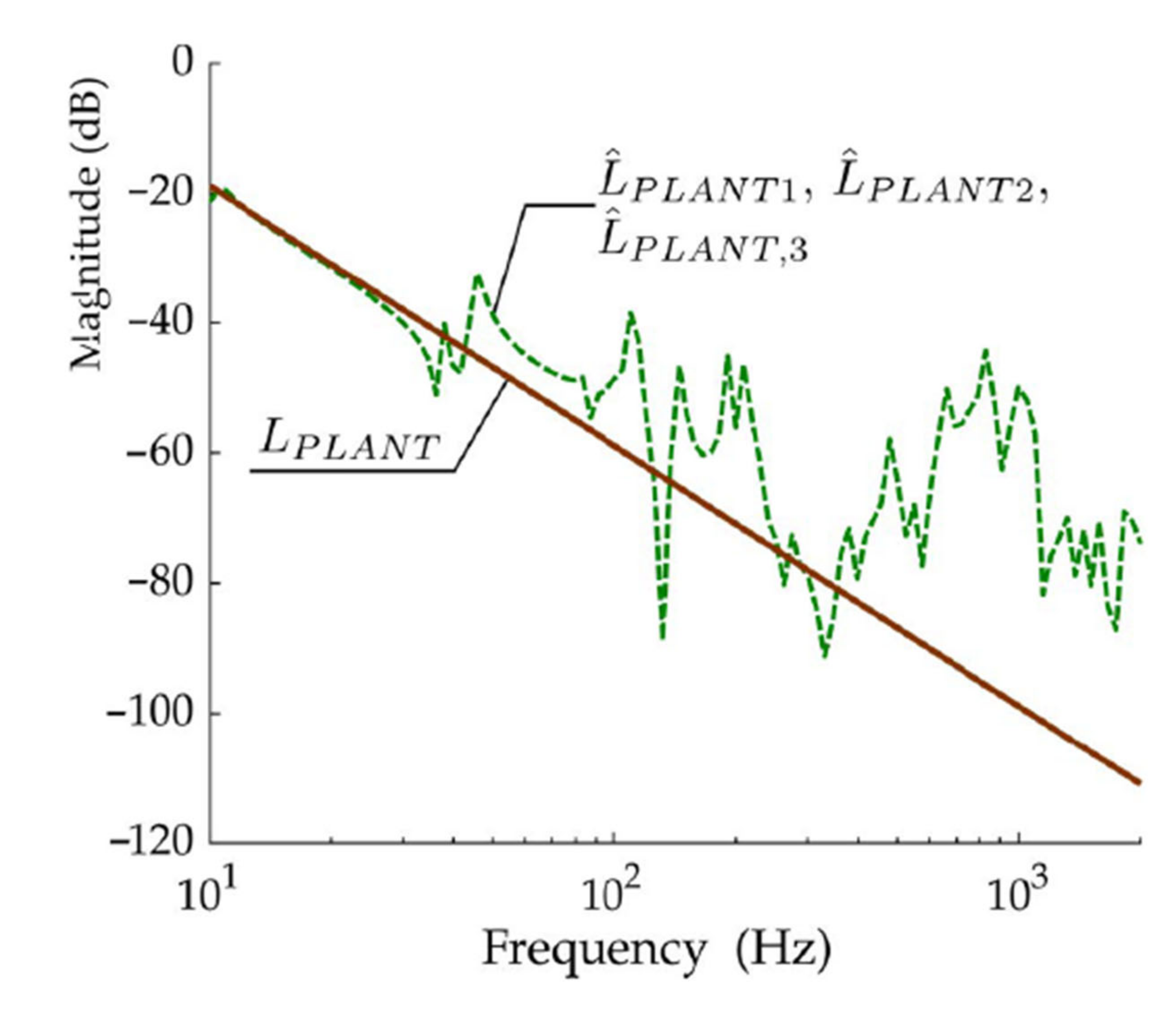
An excitation of the system with the harmonic signal of the constant amplitude to identify the transfer functions of the systems under investigation. This investigation gives the information concerning the frequency domain.

(2)

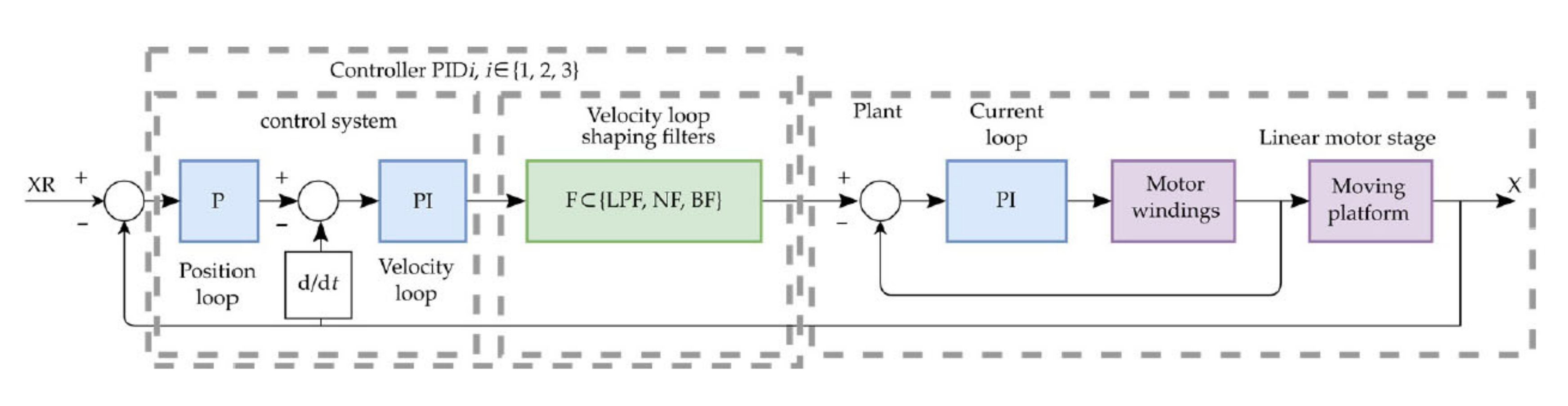
Tuning of the system to adjust the velocity loop shaping filters.

(3)

Excitation of the moving part of LMS by different velocities.

(4)

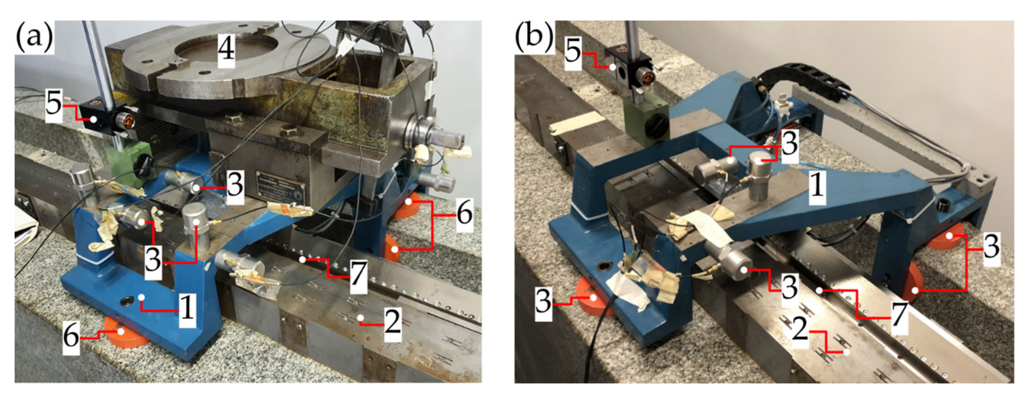
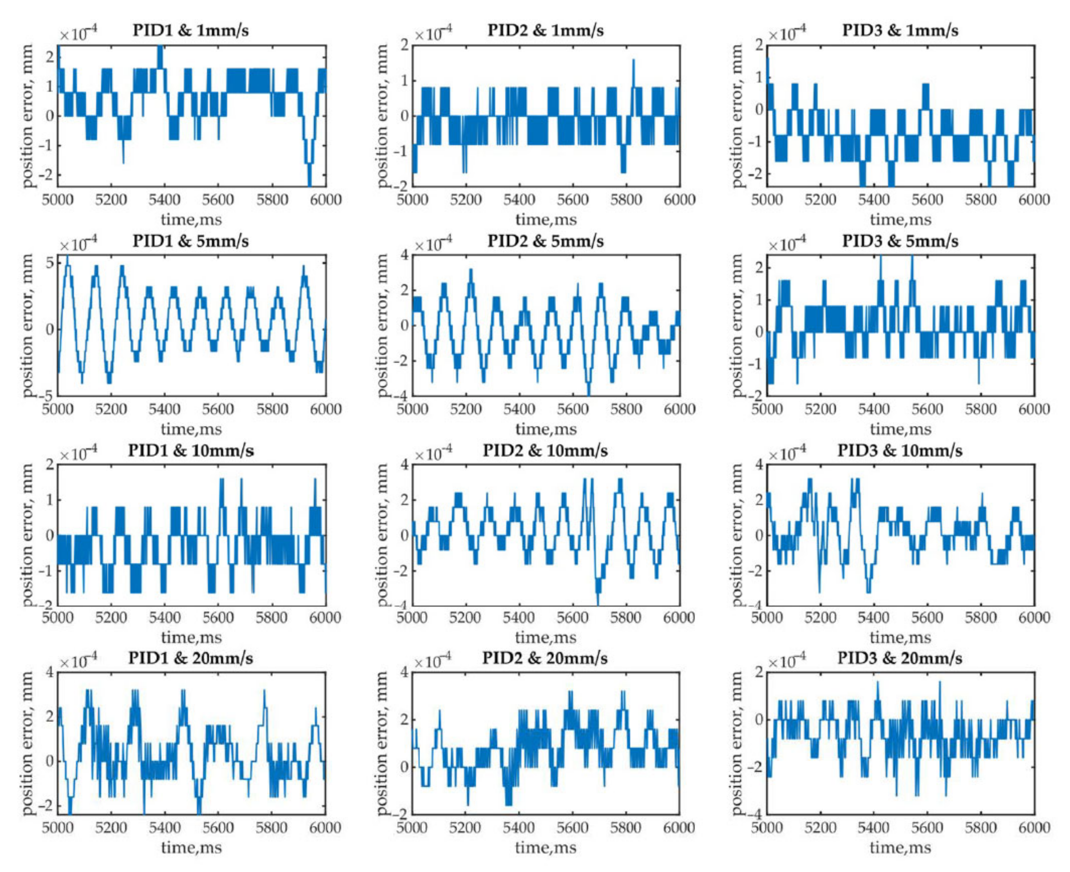
Analysis of the time dependent displacement of the moving platform, see detail 1 in Figure 1, at steady dynamic process ($\ddot{x}$ = 0) as a function of the different velocities $\dot{x}\in \left\{1,5,10,20\right\}$ mm/s and different controllers: PID1, PID2 and PID3, while the mass of load $m_{tot}\approx 100$ kg was constant.

Firstly, the direct measurement of the dynamic error of the displacement of the LMS platform has been performed. The error of the displacement, denoted by ${\Delta }_e$, in this article is expressed hereafter as a difference ${\Delta }_e={\Delta }_m-{\Delta }_{set}$, where ${\Delta }_m$ is the measured displacement and ${\Delta }_{set}$ is the required displacement set by the computer. The dynamic displacement errors ${\Delta }_e$ of the systems with the different controllers PID1, PID2 and PID3 and at the different velocities $\dot{x}\in \left\{1,5,10,20\right\}$ mm/s, at the constant acceleration $\ddot{x}=0$ of the moving platform, are shown in Figure 11.

As we can see from Figure 11, the dependency of the displacement dynamic error ${\Delta }_e$ on the time is harmonic. The displacement error ${\Delta }_e$ is smaller at the low excitation velocities, i.e., when $\dot{x}\in \left\{1,5\right\}$ mm/s in comparison to the error ${\Delta }_e$ at the bigger excitation velocities, when $\dot{x}\in \left\{10,20\right\}$ mm/s. The influence of the complexity of controller PID on the dynamic errors ${\Delta }_e$ is bigger at the low velocity than at the big velocity.

In

Table 2. Estimations of the dynamic displacement error ${\Delta }_e$ of the LMS platform.

Controller
	PID1				PID2				PID3
Estimations of the dynamic displacement error, ${\Delta }_e$ in nm
Velocity, mm/s	min{Δe}	max{Δe}	$s_{\Delta }{}_e$	$m_{\Delta }{}_e$	min{Δe}	max{Δe}	$s_{\Delta }{}_e$	$m_{\Delta }{}_e$	min{Δe}	max{Δe}	$s_{\Delta }{}_e$	$m_{\Delta }{}_e$
1	−240.00	240.00	79.70	58.20	−160.00	160.00	50.60	−14.20	−240.00	160.00	65.10	−79.03
5	−400.00	560.00	213.00	51.80	−400.00	320.00	140.00	−37.50	−160.00	240.00	63.30	21.10
10	−160.00	160.00	66.50	−30.50	−400.00	320.00	130.00	26.70	−320.00	320.00	122.00	15.90
20	−240.00	320.00	117.00	31.70	−160.00	320.00	92.10	75.80	−320.00	160.00	85.30	−62.70

, the estimations are summarized of the dynamic displacement error ${\Delta }_e$ of the LMS platform with different controllers PID1, PID2 and PID3 at different velocities $\dot{x}\in \left\{1,5,10,20\right\}$ mm/s and at the constant acceleration $\ddot{x}=0$. In this table, the estimations of mean, standard deviation, minimum and maximum are denoted by $m_{\Delta }{}_e$, $s_{\Delta }{}_e$, $min$ and $max$, respectively.

From Table 2, we can observe the following minimums of the absolute value of the estimated means, $min\left\{\left|m_{\Delta }{}_e\right|\right\}:=min\left\{\left|m_{\Delta }{}_{e,i}\right|:i\in \left\{PID1,PID2,PID3\right\}\right\}$, and the estimated standard deviation, $min\left\{s_{\Delta }{}_e\right\}:=min\left\{s_{\Delta }{}_{e,i}i:i\in \left\{PID1,PID2,PID3\right\}\right\}$, of the dynamic error ${\Delta }_e$ depending on the velocity $\dot{x}\in \left\{1,5,10,20\right\}$ mm/s, at the constant acceleration $\ddot{x}=0$ m/s²:

(1)

When the velocity $\dot{x}=1$ m/s, the LMS with controller PID2 attains both minimum values $min\left\{m_{{\Delta }_e}\right\}=\left|m_{{\Delta }_{e,PID2}}\right|=14.2$ nm and $min\left\{s_{\Delta }{}_e\right\}=s_{{\Delta }_{e,PID2}}=50.6$ nm.

(2)

When the velocity $\dot{x}=5$ m/s, the LMS with controller PID3 attains both minimum values $min\left\{\left|m_{{\Delta }_e}\right|\right\}=\left|m_{{\Delta }_{e,PID3}}\right|=21.1$ nm and $min\left\{s_{\Delta }{}_e\right\}=s_{{\Delta }_{e,PID3}}=63.3$ nm.

(3)

When the velocity $\dot{x}=10$ m/s, the LMS with controller PID3 attains minimum values of the estimated mean $min\left\{\left|m_{\Delta }{}_e\right|\right\}=m_{{\Delta }_{e,PID3}}\vee 19.9$ nm, while the LMS with PID1 attains the minimum estimated standard deviation: $min\left\{s_{\Delta }{}_e\right\}=s_{{\Delta }_{e,PID1}}=31.7$ nm.

(4)

When the velocity $\dot{x}=20$ m/s, the LMS with controller PID1 attains minimum values of the estimated mean $min\left\{\left|m_{\Delta }{}_e\right|\right\}=\left|m_{{\Delta }_{e,PID1}}\right|=66.5$ nm, while the LMS with PID3 attains the minimum estimated standard deviation: $min\left\{s_{\Delta }{}_e\right\}=s_{{\Delta }_{e,PID3}}=85.3$ nm.

The following conclusions can be made from the obtained dynamic errors ${\Delta }_e$ of the displacements of the LMS platform. In general, there is no explicit tendency that the more complex controllers provide smaller dynamic errors of the displacement ${\Delta }_e$. For example, when $\dot{x}=20$ mm/s, the smallest estimation of the absolute value of the mean of ${\Delta }_e$ is obtained for LMS with relatively simple controller PID1, i.e., $min\left\{\left|m_{{\Delta }_e}\right|\right\}=\left|m_{{\Delta }_{e,PID1}}\right|$. However, the measured dynamic errors ${\Delta }_e$ show that the complexity of the controller decreases with the increase of the velocity. Additionally, it can be stated that the relative simple controller PID1 is good enough to stabilize the displacements of the LMS moving platform at all considered velocities $\dot{x}\in \left\{1,5,10,20\right\}$ mm/s. It should be noticed that the transfer function of LMS with PID1, i.e., $H_{OLSYS1}$, is relatively simple in comparison to other transfer functions $H_{OLSYS2}$ and $H_{OLSYS3}$. The nominator of $H_{OLSYS1}$ is the polynomial of the fourth order, while its denominator is the polynomial of the eighth order. Contrarily, the polynomial of the denominator of $H_{OLSYS3}$ is even of 12th order.

5. Conclusions

The linear motor stage based on the symmetric linear motor was analyzed. The dynamic errors of the displacement of the platform of the one degree of freedom long-travel linear motor stage have been investigated by applying three different controllers consisting of a low pass filter, notch filter and the second-order bi-quad filter at four different excitation velocities 1, 5, 10 and 20 mm/s and at the steady-state, i.e., when the acceleration equals 0.

The following conclusions can be made on the bases of the obtained experimental and analytical results and their analysis:

(1)

To decrease the dynamic displacement error of the platform, the order of the polynomials of the transfer function of the considered long-travel linear motor stage should be increased with the decreased velocity of the displacements of the stage;

(2)

The transfer functions of the fourth order polynomials can be good enough to obtain an appropriate dynamic error of the displacement of the platform when the velocity of the platform is 10 mm/s and 20 mm/s;

(3)

The minimums of the estimated mean and the standard deviation of the dynamic displacement error of the platform were attained with the following controllers depending on the exciting velocity:

• At 1 mm/s exciting velocity, the best controller consists of low pass and notch filters (controller PID2); the absolute value of the estimated mean and the standard deviation are 14.2 nm and 50.6 nm, respectively;
• At 5 mm/s exciting velocity, the best controller consists of only one low pass filter (controller PID1); the estimated mean and the standard deviation are 21.1 nm and 63.3 nm, respectively;
• At 10 mm/s exciting velocity, according to the estimated standard deviation of the dynamic error, the best controller consists of one low pass filter (controller PID1); the standard deviation is 66.5 nm. However, according to the estimated mean, the best controller consists of a low pass filter, notch filter and second-order bi-quad filter (controller PID3); the estimated mean is 15.9 nm.
• At 20 mm/s exciting velocity, according to the estimated standard deviation of the dynamic error, the best controller consists of a low pass filter, notch filter and second-order bi-quad filter (controller PID3); the standard deviation is 85.3 nm. However, according to the estimated mean, the best controller consists only of a low pass filter (controller PID1); the estimated mean is 31.7 nm.

References

1. Fan, Y.; Shao, J.; Sun, G. Optimized PID Controller Based on Beetle Antennae Search Algorithm for Electro-Hydraulic Position Servo Control System. Sensors 2019, 19, 2727. [Google Scholar] [CrossRef] [PubMed] [Green Version]
2. Gao, B.; Shao, J.; Yang, X. A compound control strategy combining velocity compensation with ADRC of electro-hydraulic position servo control system. ISA Trans. 2014, 53, 1910–1918. [Google Scholar] [CrossRef] [PubMed]
3. Chen, X.; Zhong, W.; Li, C.; Fang, J.; Liu, F. Development of a Contactless Air Conveyor System for Transporting and Positioning Planar Objects. Micromachines 2018, 9, 487. [Google Scholar] [CrossRef] [PubMed] [Green Version]
4. Gao, Q.; Chen, W.; Lu, L.; Huo, D.; Cheng, K. Aerostatic bearings design and analysis with the application to precision engineering: State-of-the-art and future perspectives. Tribol. Int. 2019, 135, 1–17. [Google Scholar] [CrossRef]
5. Nishio, U.; Somaya, K.; Yoshimoto, S. Numerical calculation and experimental verification of static and dynamic characteristics of aerostatic thrust bearings with small feedholes. Tribol. Int. 2011, 44, 1790–1795. [Google Scholar] [CrossRef]
6. Sung, E.; Seo, C.-H.; Song, H.; Choi, B.; Jeon, Y.; Choi, Y.-M.; Kim, K.; Lee, M.G. Design and experiment of noncontact eddy current damping module in air bearing–guided linear motion system. Adv. Mech. Eng. 2019, 11, 168781401987142. [Google Scholar] [CrossRef] [Green Version]
7. Chang, K.-M. Design of adaptive sliding mode controller for chaos synchronization. In Proceedings of the 2007 Mediterranean Conference on Control & Automation, Institute of Electrical and Electronics Engineers (IEEE), Athens, Greece, 27–29 June 2007; pp. 1–5. [Google Scholar]
8. Rajagopal, K.; Laarem, G.; Karthikeyan, A.; Srinivasan, A.K. FPGA implementation of adaptive sliding mode control and genetically optimized PID control for fractional-order induction motor system with uncertain load. Adv. Differ. Eq. 2017, 2017, 273. [Google Scholar] [CrossRef] [Green Version]
9. Yang, X.; Liu, H.; Xiao, J.; Zhu, W.; Liu, Q.; Gong, G.; Huang, T. Continuous Friction Feedforward Sliding Mode Controller for a TriMule Hybrid Robot. IEEE/ASME Trans. Mechatron. 2018, 23, 1673–1683. [Google Scholar] [CrossRef]
10. Jiang, W.; Wang, H.; Lu, J.; Cai, G.; Qin, W. Synchronization for chaotic systems via mixed-objective dynamic output feedback robust model predictive control. J. Frankl. Inst. 2017, 354, 4838–4860. [Google Scholar] [CrossRef]
11. Taleb, M.; Plestan, F. Adaptive robust controller based on integral sliding mode concept. Int. J. Control. 2016, 89, 1788–1797. [Google Scholar] [CrossRef]
12. Yan, X.; Estrada, A.; Plestan, F. Adaptive Pulse Output Feedback Controller Based on Second-Order Sliding Mode: Methodology and Application. IEEE Trans. Control. Syst. Technol. 2016, 24, 2233–2240. [Google Scholar] [CrossRef] [Green Version]
13. Bourogaoui, M.; Sethom, H.B.A.; Belkhodja, I.S. Speed/position sensor fault tolerant control in adjustable speed drives—A review. ISA Trans. 2016, 64, 269–284. [Google Scholar] [CrossRef] [PubMed]
14. Campa, R.; Kelly, R.; Santibáñez, V. Windows-based real-time control of direct-drive mechanisms: Platform description and experiments. Mechatronics 2004, 14, 1021–1036. [Google Scholar] [CrossRef]
15. Gamazo-Real, J.C.; Vázquez-Sánchez, E.; Gomez-Gil, J. Position and Speed Control of Brushless DC Motors Using Sensorless Techniques and Application Trends. Sensors 2010, 10, 6901–6947. [Google Scholar] [CrossRef] [Green Version]
16. Gan, M.-G.; Zhang, M.; Zheng, C.-Y.; Chen, J. An adaptive sliding mode observer over wide speed range for sensorless control of a brushless DC motor. Control. Eng. Proc. 2018, 77, 52–62. [Google Scholar] [CrossRef]
17. Liu, X.; Liu, C.; Pong, P.W.T. Velocity Measurement Technique for Permanent Magnet Synchronous Motors Through External Stray Magnetic Field Sensing. IEEE Sens. J. 2018, 18, 4013–4021. [Google Scholar] [CrossRef]
18. Malikan, M.; Eremeyev, V.A.; Żur, K.K. Effect of Axial Porosities on Flexomagnetic Response of In-Plane Compressed Piezomagnetic Nanobeams. Symmetry 2020, 12, 1935. [Google Scholar] [CrossRef]
19. Lingling, Y.; Zhuo, M.; Jianqiu, B.; Yize, S. Non-Linear Dynamic Feature Analysis of a Multiple-Stage Closed-Loop Gear Transmission System for 3D Circular Braiding Machine. Symmetry 2020, 12, 1788. [Google Scholar]
20. Cheng-Chi, W.; Chih-Jer, L. Bifurcation and Nonlinear Behavior Analysis of Dual-Directional Coupled Aerodynamic Bearing Systems. Symmetry 2020, 12, 1521. [Google Scholar]
21. Das, S.; Nandi, D.; Neogi, B.; Sarkar, B. Nonlinear System Stability and Behavioral Analysis for Effective Implementation of Artificial Lower Limb. Symmetry 2020, 12, 1727. [Google Scholar] [CrossRef]
22. Ammar, A.; Kheldoun, A.; Metidji, B.; Ameid, T.; Azzoug, Y. Feedback linearization based sensorless direct torque control using stator flux MRAS-sliding mode observer for induction motor drive. ISA Trans. 2020, 98, 382–392. [Google Scholar] [CrossRef] [PubMed]
Figure 1. The general view of the long travel linear motor stage with the air bearings with load (a) and without load (b): 1 is the moving platform; 2 is the granite base; 3 are the accelerometers; 4 is the load; 5 is the interferometer mirror; 6 are the air bearings; and 7 is the three-phase linear BLDC motor “TECNOTION UM9N.”
Symmetry 12 02062 g001
Figure 2. The general view of the test equipment: 1 is the granite base; 2 is the Michelson interferometer RENISHAW XL-80; 3 is the long travel linear motor stage with the air bearings (LMS); 4 is the PC with control and diagnostic software; 5 is the setup based on controller ACS SP + EC-04000032NAN5NDNN and motor driver (current amplifier) ACS UDMSD2B2N0N.
Symmetry 12 02062 g002
Figure 3. The block diagram of the long travel linear motor stage with air bearings (LMS).
Symmetry 12 02062 g003
Figure 4. Frequency response functions of the plant: L ^ P L A N T i , i 1 , 2 , 3 are the experimentally identified FRF and L P L A N T is the FRF of the theoretical transfer function H P L A N T given in Equation (6).
Symmetry 12 02062 g004
Figure 5. Frequency response functions of controller PID1: L ^ P I D 1 is the experimentally identified FRF and L P I D 1 is the FRF of the theoretical transfer function H P I D 1 given in Equation (7).
Symmetry 12 02062 g005
Figure 6. Frequency response functions of controller PID2: L ^ P I D 2 is the experimentally identified FRF and L P I D 2 is the FRF of the theoretical transfer function H P I D 2 given in Equation (8).
Symmetry 12 02062 g006
Figure 7. Frequency response functions of controller PID3: L ^ P I D 3 is the experimentally identified FRF and L P I D 3 is the FRF of the theoretical transfer function H P I D 3 given in Equation (9).
Symmetry 12 02062 g007
Figure 8. Experimentally and analytically obtained FRFs, L ^ O L S Y S 1 and L O L S Y S 1 , respectively, of LMS with controller PID2.
Symmetry 12 02062 g008
Figure 9. Experimentally and analytically obtained FRFs, L ^ O L S Y S 2 and L O L S Y S 2 , respectively, of LMS with controller PID2.
Symmetry 12 02062 g009
Figure 10. Experimentally and analytically obtained FRFs, L ^ O L S Y S 3 and L O L S Y S 3 , respectively, of LMS with controller PID3.
Symmetry 12 02062 g010
Figure 11. Dynamic displacement errors Δ e of the LMS platform with different controllers PID1, PID2 and PID3 at different velocities x ˙ 1 , 5 , 10 , 20 mm/s and at the constant acceleration x ¨ = 0 .
Symmetry 12 02062 g011