Article

Utilizing Macro Fiber Composite to Control Rotating Blade Vibrations

1
Department of Mathematics and Statistics, College of Science, Taif University, P.O. Box 11099, Taif 21944, Saudi Arabia
2
Department of Physics and Engineering Mathematics, Faculty of Electronic Engineering, Menoufia University, Menouf 32952, Egypt
3
Institute of Engineering, Polytechnic of Porto, Rua Dr. António Bernardino de Almeida, 431, 4249-015 Porto, Portugal
*
Authors to whom correspondence should be addressed.
Symmetry 2020, 12(12), 1984; https://doi.org/10.3390/sym12121984
Submission received: 30 October 2020 / Revised: 26 November 2020 / Accepted: 27 November 2020 / Published: 30 November 2020

Abstract

:
This work applies an active control algorithm, using a macro fiber composite (MFC) to mitigate the unwanted vibrations of a rotating blade. The algorithm is a second-order oscillator, having the positive displacement signal of the blade for input and the suitable control force to actuate the blade for output. This oscillator is linearly coupled with the blade, having in mind that their natural frequencies must be in the vicinity of each other. The rotating blade is modeled by representing two vibrational directions that are linearly coupled. An asymptotic analysis is considered to understand the resulting nonlinear phenomena. Several responses are included to portray the dynamical behavior of the system under control. From the results, we observe the asymmetry between the blade’s vibrational directions. Moreover, a verification is included for comparing the analytical and numerical results.

1. Introduction

Rotating blades are important structures, being fundamental in many industrial fields like robotics, aerospace engineering, turbomachinery, and others. Due to their high rotating speeds, they may suffer from unwanted oscillations, causing disturbance and damage to, or even destruction of, the whole mechanism. Consequently, many researchers have focused their attention on the analysis and control of these vibrations to achieve maximum safety and optimum operation of such dynamical systems.
Yoo et al. [1] investigated, numerically, the effects of some dimensionless parameters on the vibration characteristics of a rotating blade and considered combinatory effects among these parameters. Lin and Chen [2] used a finite element analysis to study the stability problems of a rotating pre-twisted blade with a viscoelastic core constrained by a laminated face layer and subjected to a periodic axial load. They derived a system of equations of motion, governing the bending and extensional displacements through the Hamilton principle. Oh et al. [3] developed a structural beam model accounting for the fibrous composite material effects and the induced elastic couplings. Librescu et al. [4] considered the modeling of a spinning, thin-walled beam made of functionally graded materials, featuring a pre-twist and experiencing bending–bending coupled motion. Sinha [5] derived a complete set of coupled dynamic equations to analyze the effect of a Coulomb damper near the blade tip with a flexible blade mounted on a flexible rotating shaft. Hamdan and El-Sinawi [6] developed a slender, flexible arm dynamic model undergoing relatively large planar flexural deformations with a setting angle and a rotating hub. They derived the model by assuming an inextensible Euler–Bernoulli beam while taking into account the axial inertia and nonlinear curvature.
Other researchers focused on controlling the thin-walled rotating blades via other advanced techniques. Choi et al. [7,8] improved the damping control behavior for suppressing the vibrations of a rotating, composite, thin-walled beam by using macro fiber composite (MFC) actuators and polyvinylidene fluoride (PVDF) sensors. They performed numerical studies based on finite element analysis and investigated the dynamic responses of the beam. Fazelzadeh et al. [9] demonstrated the applicability of the differential quadrature method as an efficient numerical method for analyzing the vibrations of a rotating, thin-walled blade made of functionally graded materials. They obtained the differential quadrature’s discretized form of the governing equations and the related boundary conditions at the domain and boundary grid points. Vadiraja and Sahasrabudhe [10] described a rotating, thin-walled composite blade with embedded MFC actuators and sensors using a dynamic modeling method. Younesian and Esmailzadeh [11] concluded that the rotating blades were always subjected to a variety of external excitations due to the vortex-shedding phenomenon. In the forced vibration case, they assumed either a sinusoidal function or a random excitation with a white noise time history to be the sources of external excitation, and then investigated the behavior of the passively controlled blade.
Some researchers worked on controlling the vibration behavior by adjusting the blade’s physical parameters. Yao et al. [12,13] investigated the complex dynamics and adopted a numerical approach to analyze the periodic and chaotic motions of a rotating blade. They could control the blade responses, changing from chaotic to periodic behavior, by adjusting the rotating speed. Latalski [14] discussed the dynamics of a rotating rigid hub with a flexible, composite, thin-walled blade by taking into account the moment of inertia of the hub mass. Rafiee et al. [15] presented a comprehensive review of articles about rotating composite blades that were published in recent decades. The review addressed analytical, semi-analytical, and numerical studies dealing with dynamical problems involving adaptive, smart, or intelligent materials. Chen and Li [16] presented a dynamic model based on the shell theory to investigate the vibration behavior of a pre-twisted, rotating, composite, laminated blade. They considered the effects of Coriolis and centrifugal forces, due to the rotation motion of the blade. Liu and Gong [17] proposed a theoretical model and vibration control for the divergent motion of a thin-walled, pre-twisted wind turbine blade based on a linear quadratic Gaussian controller. Zhang et al. [18,19,20] studied the saturation phenomena and the primary resonance of a rotating, pre-twisted, laminated, composite blade subjected to a subsonic airflow excitation, using the Vortex lattice method in the case of 1 : 2 internal resonance.
Concerning the use of MFC, Wang et al. [21] proposed a reliability-based design optimization approach for improving the buckling load of variable angle tow filament-wound cylinders subject to axial compression. They showed a fast convergence by the metamodel, achieving an efficient computational optimization for all cases. Almeida et al. [22] evaluated, both experimentally and numerically, the notched strength and longitudinal tensile characteristics in unnotched and notched composites. The notched strength decreased by about 50% when comparing the notched and unnotched samples. Monticeli et al. [23] presented the importance of 3D characterization of the voids in composite laminates via statistical approaches. They showed that carbon fibers have more tortuosity vis-a-vis the glass fibers, which hindered flow impregnation.
Regarding active controllers, several researchers [24,25,26] controlled the vibrations of different dynamical systems using an algorithm called positive position feedback (PPF). This strategy consists of a second-order oscillator coupled to the system, which would be controlled at an internal resonance of 1 : 1 . It was verified that the PPF controller could be optimized by tuning its natural frequency to the nearby excitation frequency. Hamed et al. [27] analyzed the nonlinear vibration control of a dynamical system using a new, nonlinear modified PPF approach. The modified controller successfully suppressed the vibrational amplitude when the excitation frequency equaled the blade’s natural frequency (at σ = 0 ), and the classical PPF peaks were reduced significantly.
The motivation of this work was to merge MFC and one of the active control algorithms. The PPF active control algorithm is effective at suppressing mechanical vibrations. The role of MFC sensors is to supply the PPF controller with the feedback signal, and the role of the MFC actuators is to receive the control signal from the PPF controller. In this paper, we control the rotating blade vibrations theoretically by applying the PPF control algorithm through MFC sensors and actuators, as presented in Figure 1. The whole control process is pictured in Figure 1 to show how the MFC sensors acquired the feedback signal to be processed and conditioned, and then create a control signal to be supplied to the MFC actuators. The main difficulty was in finding a small-error approximate solution for the nonlinear model of the blade. Using the multiple scales perturbation technique, we obtained an approximate solution for the studied model in good agreement with the numerical simulations. Several response curves are included to portray the dynamical behavior of the blade under control. Moreover, a section of verification curves is included to compare the analytical and numerical results.
The rest of the paper includes three sections. Section 2 presents the equations of motion of the controlled rotating blade model and the approximate solutions to these equations. Section 3 analyzes the different response curves of the blade vibrations before and after being controlled. Moreover, verification of the responses is also included. Section 4 summarizes the conclusions of the work.

2. Equations of Motion and Their Approximate Solutions

The partial differential equations governing the horizontal and vertical deflections— p ( t ) and q ( t ) —of the blade’s cross-section were derived briefly in Appendix A and are detailed in [12,13]. The equations were discretized by a one-term Galerkin’s procedure to have the ordinary differential equations governing the temporal horizontal p ( t ) and vertical q ( t ) displacements of the blade’s cross-section. The extracted equations of motion can be written as follows:
p ¨ + 2 μ p ˙ + ω 2 p + β 13 q ˙ + β 11 q + β 5 p q 2 + β 5 p 3 = 2 f 0 f β 14 p cos ( Ω t ) + f 2 β 14 p cos 2 ( Ω t ) + f β 16 Ω sin ( Ω t )
q ¨ + 2 μ q ˙ + ω 2 q + β 22 p ˙ + β 21 p + β 5 p 2 q + β 5 q 3 = 2 f 0 f β 24 q cos ( Ω t ) + f 2 β 24 q cos 2 ( Ω t )
Applying the nonlinear PPF controller to Equation (1), the motion equations can be written as
p ¨ + 2 μ p ˙ + ω 2 p + β 13 q ˙ + β 11 q + β 5 p q 2 + β 5 p 3 = 2 f 0 f β 14 p cos ( Ω t ) + f 2 β 14 p cos 2 ( Ω t ) + f β 16 Ω sin ( Ω t ) + c 1 y
q ¨ + 2 μ q ˙ + ω 2 q + β 22 p ˙ + β 21 p + β 5 p 2 q + β 5 q 3 = 2 f 0 f β 24 q cos ( Ω t ) + f 2 β 24 q cos 2 ( Ω t )
y ¨ + 2 μ c y ˙ + ω c 2 y + α y 3 = c 2 p
The parameters of Equation (2) are suitably scaled such that
α = ε α ^ ,   β 11 = ε β ^ 11 ,   β 13 = ε β ^ 13 ,   β 14 = ε β ^ 14 ,   β 16 = ε β ^ 16 ,   β 21 = ε β ^ 21 ,   β 22 = ε β ^ 22 ,   β 24 = ε β ^ 24 ,   β 5 = ε β ^ 5 ,   c 1 ,   2 = ε c ^ 1 ,   2 ,   μ = ε μ ^ ,   μ c = ε μ ^ c
where ε is a bookkeeping parameter. If we apply the multiple scales method [28], then the asymptotic expansions of p , q , and y can be expressed as
p ( t ; ε ) = p 0 ( T 0 , T 1 ) + ε p 1 ( T 0 , T 1 ) + O ( ε 2 )
q ( t ; ε ) = q 0 ( T 0 , T 1 ) + ε q 1 ( T 0 , T 1 ) + O ( ε 2 )
y ( t ; ε ) = y 0 ( T 0 , T 1 ) + ε y 1 ( T 0 , T 1 ) + O ( ε 2 )
where T n = ε n t ( n = 0 , 1 ) are the fast and slow time scales, respectively. The time derivatives in Equation (2) can be rewritten as
d d t = D 0 + ε D 1 + O ( ε 2 )
d 2 d t 2 = D 0 2 + 2 ε D 1 D 0 + O ( ε 2 )
where D n = / T n ( n = 0 , 1 ). After inserting Equations (3)–(5) into Equation (2) and comparing the terms of ε for similar power coefficients, we get the following.
For O ( ε 0 ) :
D 0 2 p 0 + ω 2 p 0 = 0
D 0 2 q 0 + ω 2 q 0 = 0
D 0 2 y 0 + ω c 2 y 0 = 0
For O ( ε 1 ) :
D 0 2 p 1 + ω 2 p 1 = 2 D 1 D 0 p 0 2 μ ^ D 0 p 0 β ^ 13 D 0 q 0 β ^ 11 q 0 β ^ 5 p 0 q 0 2 β ^ 5 p 0 3 + f 0 f β ^ 14 p 0 ( e i Ω T 0 + e i Ω T 0 ) + f 2 β ^ 14 4 p 0 ( e i Ω T 0 + e i Ω T 0 ) 2 i f β ^ 16 Ω 2 ( e i Ω T 0 e i Ω T 0 ) + c ^ 1 y 0
D 0 2 q 1 + ω 2 q 1 = 2 D 1 D 0 q 0 2 μ ^ D 0 q 0 β ^ 22 D 0 p 0 β ^ 21 p 0 β ^ 5 p 0 2 q 0 β ^ 5 q 0 3 + f 0 f β ^ 24 q 0 ( e i Ω T 0 + e i Ω T 0 ) + f 2 β ^ 24 4 q 0 ( e i Ω T 0 + e i Ω T 0 ) 2
D 0 2 y 1 + ω c 2 y 1 = 2 D 1 D 0 y 0 2 μ ^ c D 0 y 0 α ^ y 0 3 + c ^ 2 p 0
Based upon the theory of linear differential equations, the complex form solutions of Equation (6) are
p 0 = A 1 ( T 1 ) e i ω T 0 + A ¯ 1 ( T 1 ) e i ω T 0
q 0 = A 2 ( T 1 ) e i ω T 0 + A ¯ 2 ( T 1 ) e i ω T 0
y 0 = A 3 ( T 1 ) e i ω c T 0 + A ¯ 3 ( T 1 ) e i ω c T 0
Preliminary numerical simulations of the controlled blade model revealed that the worst resonance occurred for cases where Ω ω and ω c ω . Therefore, the parameters σ 1 and σ 2 were imposed to express the detuning of the considered resonance case so that
Ω = ω + σ 1
ω c = ω + σ 2
To avoid any unbounded solutions, and from the theory of linear differential equations, we can eliminate the secular terms in Equation (7) by equalizing the coefficients of e i ω T 0 and e i ω c T 0 to zero. Equations (8) and (9) are inserted into Equation (7). Then, using Equation (3), we can return every parameter to the real time t , which leads to
2 i ω A ˙ 1 2 i μ ω A 1 i ω β 13 A 2 β 11 A 2 2 β 5 A 1 A 2 A ¯ 2 β 5 A ¯ 1 A 2 2 3 β 5 A 1 2 A ¯ 1 + β 14 f 2 2 A 1 + β 14 f 2 4 A ¯ 1 e 2 i σ 1 t i 2 β 16 Ω f e i σ 1 t + c 1 A 3 e i σ 2 t = 0
2 i ω A ˙ 2 2 i μ ω A 2 i ω β 22 A 1 β 21 A 1 2 β 5 A 1 A ¯ 1 A 2 β 5 A 1 2 A ¯ 2 3 β 5 A 2 2 A ¯ 2 + β 24 f 2 2 A 2 + β 24 f 2 4 A ¯ 2 e 2 i σ 1 t = 0
2 i ω c A ˙ 3 2 i μ c ω c A 3 3 α A 3 2 A ¯ 3 + c 2 A 1 e i σ 2 t = 0
The functions A n ( n = 1 , 2 , 3 ) can be formulated in a polar form as
A n = a n 2 e i δ n A ˙ n = a ˙ n 2 e i δ n + i a n 2 δ ˙ n e i δ n
where an and δn are the amplitudes and phases of the blade vibrational directions and controller signal, respectively. Inserting Equation (11) into Equation (10), separating real and imaginary parts, and simplification gives us
a ˙ 1 = μ a 1 β 13 2 a 2 cos ϕ 2 β 11 2 ω a 2 sin ϕ 2 β 5 8 ω a 1 a 2 2 sin ( 2 ϕ 2 ) + β 14 f 2 8 ω a 1 sin ( 2 ϕ 1 ) β 16 Ω f 2 ω cos ϕ 1 + c 1 2 ω a 3 sin ϕ 3
ϕ ˙ 1 = σ 1 + β 13 2 a 2 a 1 sin ϕ 2 β 11 2 ω a 2 a 1 cos ϕ 2 β 5 4 ω a 2 2 β 5 8 ω a 2 2 cos ( 2 ϕ 2 ) 3 β 5 8 ω a 1 2 + β 14 f 2 8 ω cos ( 2 ϕ 1 ) + β 14 f 2 4 ω + β 16 Ω f 2 ω 1 a 1 sin ϕ 1 + c 1 2 ω a 3 a 1 cos ϕ 3
a ˙ 2 = μ a 2 β 22 2 a 1 cos ϕ 2 + β 5 8 ω a 1 2 a 2 sin ( 2 ϕ 2 ) + β 24 f 2 8 ω a 2 sin ( 2 ϕ 1 2 ϕ 2 ) + β 21 2 ω a 1 sin ϕ 2
ϕ ˙ 2 = β 22 2 a 1 a 2 sin ϕ 2 + β 21 2 ω a 1 a 2 cos ϕ 2 + β 5 4 ω   a 1 2   + β 5   8 ω a 1 2 cos ( 2 ϕ 2 ) + 3 β 5 8 ω a 2 2 β 24 f 2 8 ω cos ( 2 ϕ 1 2 ϕ 2 ) β 24 f 2 4 ω + β 13   2 a 2 a 1 sin ϕ 2 β 11   2 ω a 2 a 1 cos ϕ 2 β 5 4 ω   a 2 2   β 5   8 ω a 2 2 cos ( 2 ϕ 2 ) 3 β 5 8 ω a 1 2 + β 14 f 2 8 ω cos ( 2 ϕ 1 ) + β 14 f 2 4 ω + β 16 Ω f   2 ω 1 a 1 sin ϕ 1 + c 1 2 ω a 3 a 1 cos ϕ 3
a ˙ 3 = μ c a 3 c 2 2 ω c a 1 sin ϕ 3
ϕ ˙ 3 = σ 2 + 3 α 8 ω c a 3 2 c 2 2 ω c a 1 a 3 cos ϕ 3 + β 13 2 a 2 a 1 sin ϕ 2 β 11 2 ω a 2 a 1 cos ϕ 2 β 5 4 ω a 2 2 β 5 8 ω a 2 2 cos ( 2 ϕ 2 ) 3 β 5 8 ω a 1 2 + β 14 f 2 8 ω cos ( 2 ϕ 1 ) + β 16 Ω f 2 ω 1 a 1 sin ϕ 1 + β 14 f 2 4 ω + c 1 2 ω a 3 a 1 cos ϕ 3
where ϕ 1 = σ 1 t δ 1 , ϕ 2 = δ 2 δ 1 , and ϕ 3 = σ 2 t + δ 3 δ 1 .   The steady-state form of Equation (12) can be reached by imposing the condition that a ˙ n = ϕ ˙ n = 0 ( n = 1 , 2 , 3 ), but the resulting expressions cannot be solved explicitly, at which point we should resort to the Newton–Raphson numerical technique. A stability analysis needs to be done to examine whether the steady-state solutions are stable or not. Suppose that the amplitudes a n are composed of perturbation amplitudes a n p added to the steady-state amplitudes a n s . Similarly, suppose that the phases ϕ n are composed of perturbation phases ϕ n p added to the steady-state phases ϕ n s . This can be formulated as follows:
a n = a n p + a n s a ˙ n = a ˙ n p
ϕ n = ϕ n p + ϕ n s ϕ ˙ n = ϕ ˙ n p
Inserting Equation (13) into Equation (12) and linearizing give us
( a ˙ 1 p ϕ ˙ 1 p a ˙ 2 p ϕ ˙ 2 p a ˙ 3 p ϕ ˙ 3 p ) = J ( a 1 p ϕ 1 p a 2 p ϕ 2 p a 3 p ϕ 3 p ) = ( r 11 r 12 r 13 r 14 r 15 r 16 r 21 r 22 r 23 r 24 r 25 r 26 r 31 r 32 r 33 r 34 r 35 r 36 r 41 r 42 r 43 r 44 r 45 r 46 r 51 r 52 r 53 r 54 r 55 r 56 r 61 r 62 r 63 r 64 r 65 r 66 ) ( a 1 p ϕ 1 p a 2 p ϕ 2 p a 3 p ϕ 3 p )
where J is the Jacobian matrix whose elements are given in Appendix B. The characteristic equation of J is a sixth degree equation in the following form:
λ 6 + γ 1 λ 5 + γ 2 λ 4 + γ 3 λ 3 + γ 4 λ 2 + γ 5 λ + γ 6 = 0
where γ i ( i = 1 , , 6 ) are given in Appendix B. The roots λ of Equation (15) are the eigenvalues of J , and they determine whether the system solutions are stable or not. If the real parts of the eigenvalues λ are negative, then the steady state solution will be asymptotically stable; otherwise, it will be unstable. To guarantee the stability of the solutions, the Routh–Hurwitz theorem is considered to derive the criteria for stable solutions:
( γ 1 ) ( γ 1 γ 2 γ 3 ) ( γ 1 2 γ 4 + γ 1 γ 2 γ 3 + γ 1 γ 5 γ 3 2 ) ( γ 1 2 γ 2 γ 6 γ 1 2 γ 4 2 γ 1 γ 2 2 γ 5 + γ 1 γ 2 γ 3 γ 4 γ 1 γ 3 γ 6 + 2 γ 1 γ 4 γ 5 + γ 2 γ 3 γ 5 γ 3 2 γ 4 γ 5 2 ) ( γ 1 3 γ 6 2 + 2 γ 1 2 γ 2 γ 5 γ 6 + γ 1 2 γ 3 γ 4 γ 6 γ 1 2 γ 4 2 γ 5 γ 1 γ 2 2 γ 5 2 γ 1 γ 2 γ 3 2 γ 6 γ 5 3 3 γ 1 γ 3 γ 5 γ 6 + 2 γ 1 γ 4 γ 5 2 + γ 2 γ 3 γ 5 2 + γ 3 3 γ 6 γ 3 2 γ 4 γ 5 + γ 1 γ 2 γ 3 γ 4 γ 5 ) ( γ 6 ) } > 0
Moreover, if there is a sign change in a real eigenvalue, then a saddle–node bifurcation point will appear. This corresponds to the condition γ 6 = 0 . Additionally, if there is a sign change in the real parts of a pair of complex conjugate eigenvalues, then a Hopf bifurcation point will appear. This corresponds to the following conditions:
( γ 5 ) ( γ 6 ) ( γ 4 γ 5 ( γ 3 γ 6 ) ( γ 3 γ 4 γ 5 γ 2 γ 5 2 γ 3 2 γ 6 + γ 1 γ 5 γ 6 ) ( γ 2 γ 3 γ 4 γ 5 γ 1 γ 4 2 γ 5 + 2 γ 1 γ 2 γ 5 γ 6 γ 2 2 γ 5 2 + γ 4 γ 5 2 γ 3 γ 5 γ 6 γ 2 γ 3 2 γ 6 + γ 1 γ 3 γ 4 γ 6 γ 1 2 γ 6 2 ) } > 0
γ 1 γ 2 γ 3 γ 4 γ 5 γ 3 2 γ 4 γ 5 + 2 γ 1 γ 4 γ 5 2 γ 1 2 γ 4 2 γ 5 γ 1 γ 2 2 γ 5 2 + γ 2 γ 3 γ 5 2 + 2 γ 1 2 γ 2 γ 5 γ 6 γ 5 3 3 γ 1 γ 3 γ 5 γ 6 γ 1 γ 2 γ 3 2 γ 6 + γ 3 3 γ 6 + γ 1 2 γ 3 γ 4 γ 6 γ 1 3 γ 6 2 = 0

3. Results and Discussion

In this section, we analyze the different responses of the blade vibrations and the control signal to variations of the excitation frequency and force amplitude. These responses are plotted using Equations (2) and (12), with the aid of the stability criteria in Equation (16).

3.1. Effects of the Parameter Variation on the Blade Steady-State Vibrational Amplitudes
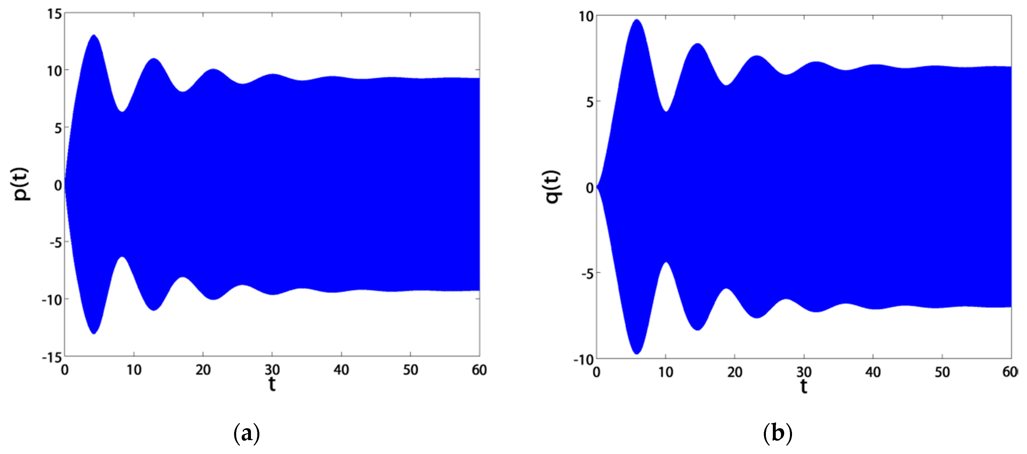
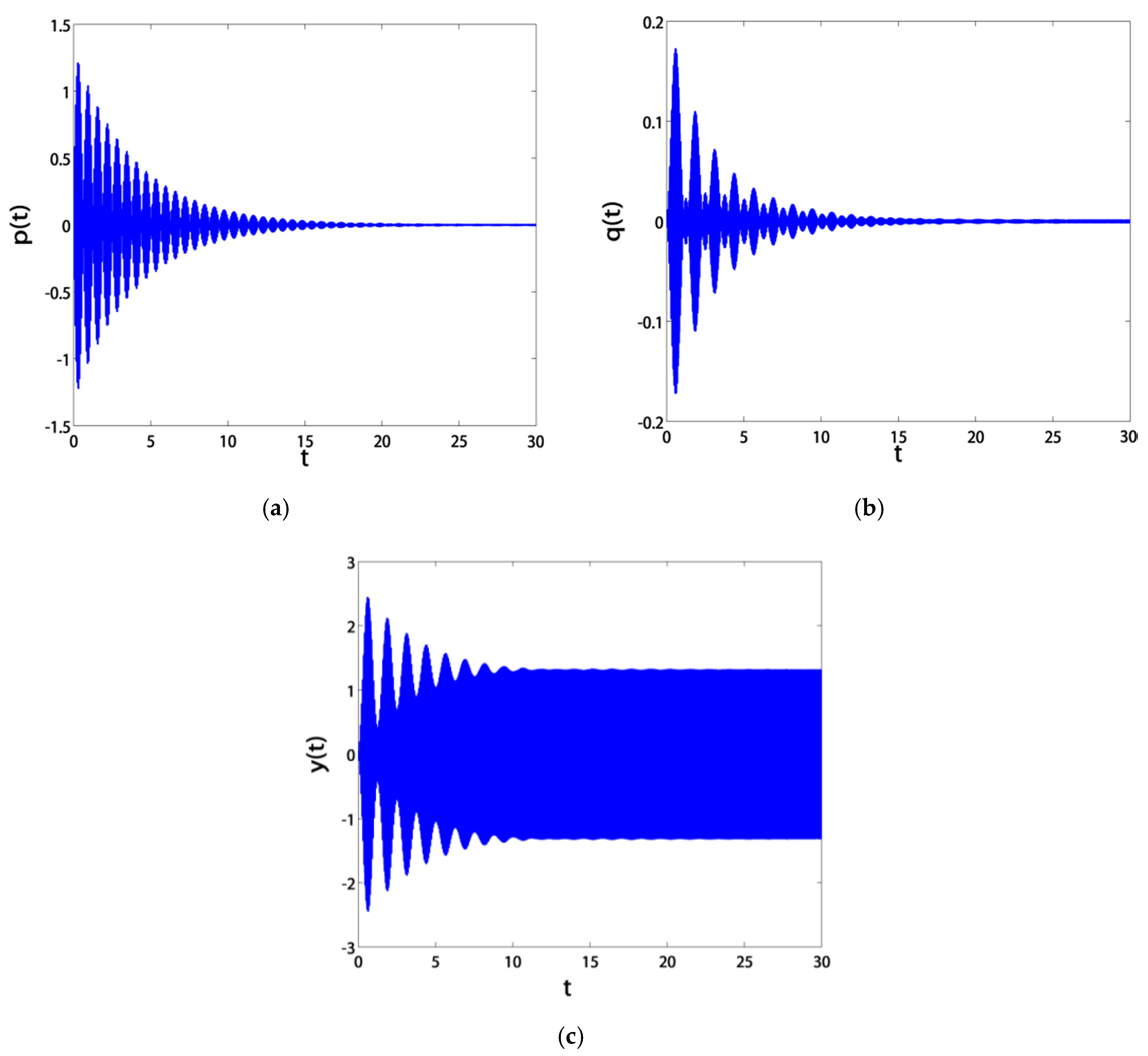
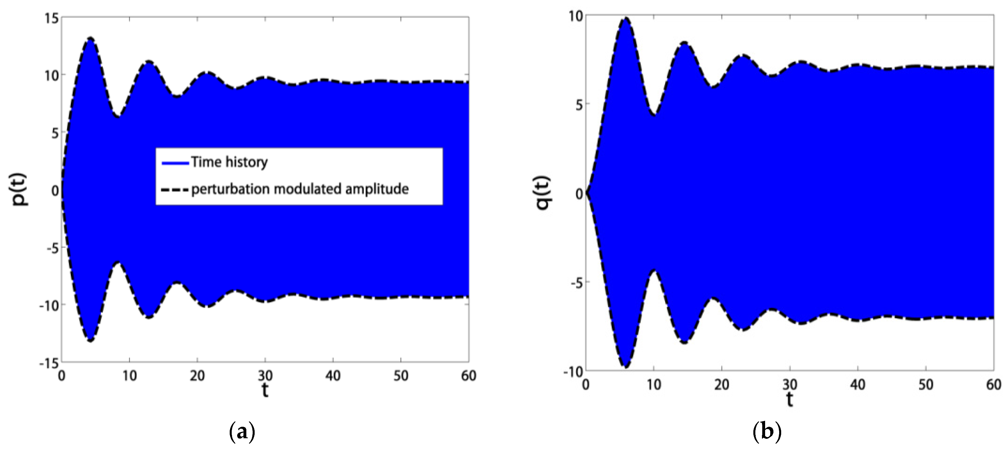
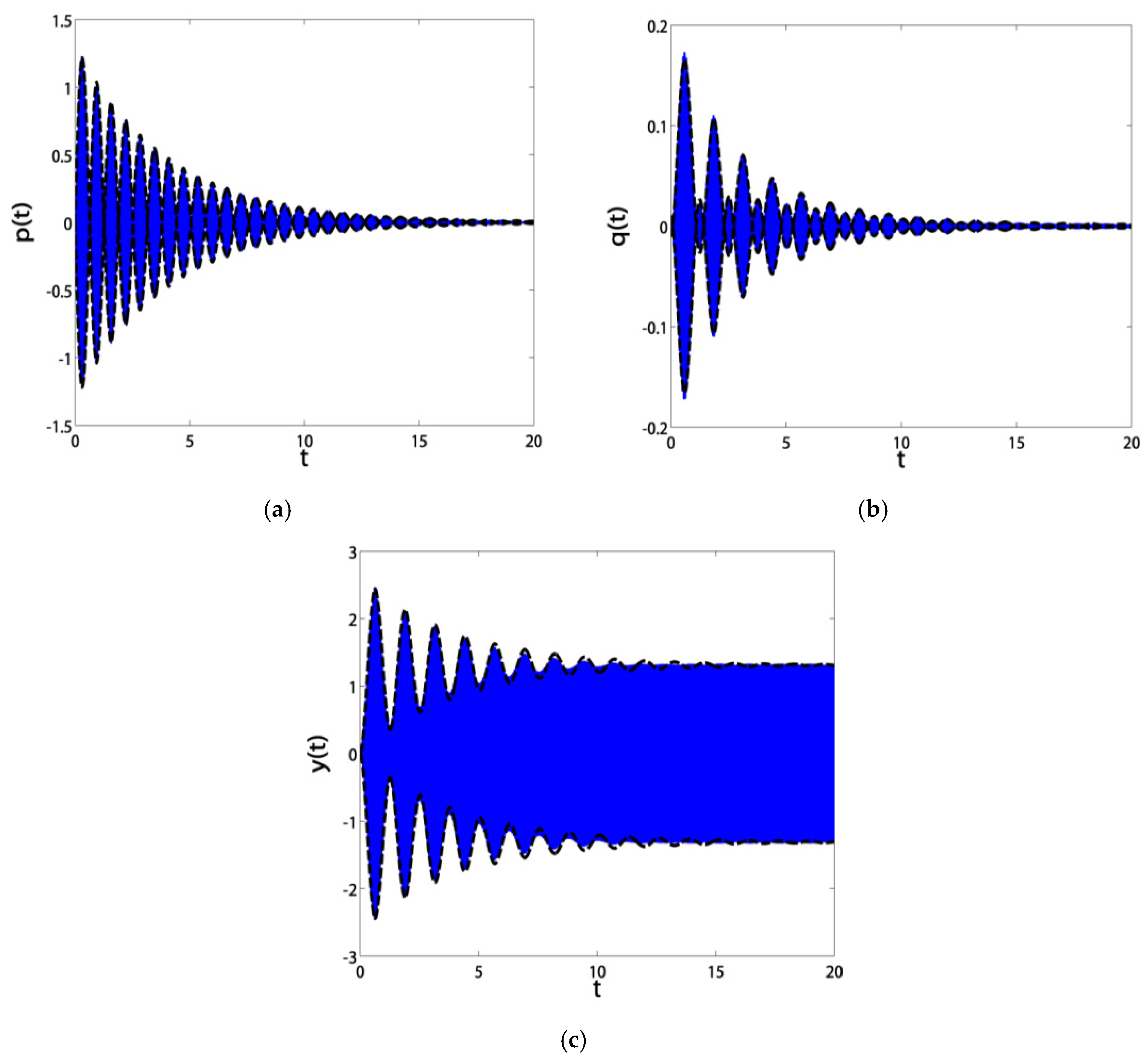
Hereafter, we adopt the parameter values μ = 0.5 , μ c = 0.005 , Ω = ω = ω c , β 11 = 0.003 , β 21 = 0.001 , β 13 = β 22 = 0.82 , β 14 = 0.55 , β 24 = 0.5 , β 5 = 0.9 , β 16 = 6.55 , f 0 = 7 , f = 2 , α = 0 , c 1 = c 2 = 1000 , and σ 1 = σ 2 = 0 . The saddle–node bifurcation and Hopf bifurcation points are denoted by SN and H, respectively. These points were explored due to the criteria in Equation (17). Figure 2 shows how the blade’s horizontal and vertical amplitude responded to the excitation frequency detuning σ 1 before control. It is clear that the blade was in a stable motion until it got into the range of 0 < σ 1 < 3 , where jumps may happen due to the existence of bifurcation points. After control, the blade’s horizontal and vertical amplitudes responded to the excitation frequency detuning σ 1 , as shown in Figure 3, achieving a stable motion all over the range of σ 1 . The bifurcation points disappeared, and no jumps were present. The blade is preferred to operate in the region of σ 1 [ 4 ,   4 ] , especially at the point σ 1 = 0 , for which the blade is at its minimum vibratory level.
Figure 4 and Figure 5 show the various effects of both the control signal gain c 1 and the feedback signal gain c 2 on the blade and controller amplitude responses to the excitation frequency detuning σ 1 . When we departed from σ 1 = 0 , the blade vibration amplitudes begin to rise. We can see the important role of c 1 and c 2 in controlling the bandwidth between the high amplitude peaks shown in the figure. This leads to increased safety if the blade’s excitation frequency Ω deviates from its natural frequency ω .
Figure 6 demonstrates the effect of the controller damping μ c on the blade and the controller responses to the excitation frequency detuning σ 1 . Increasing μ c suppressed the high amplitude peaks of the blade vibrations. However, the minimum amplitudes at σ 1 = 0 begin to rise slightly, since the energy bridge between the controller and the blade was choked.
Figure 7 shows how the variation of the controller frequency detuning σ 2 affected the blade and the controller responses to the excitation frequency detuning σ 1 . We verified that the blade and the controller were at minimum vibratory values when 5 σ 1 = σ 2 + 5 . This can be achieved only by equalizing the controller natural frequency ω c and the blade excitation frequency Ω .
Figure 8 and Figure 9 illustrate the hardening or softening effects that could be imposed on the blade and the controller responses to the excitation frequency detuning σ 1 by varying the controller nonlinearity parameter α . However, the bifurcation points, which led to the problem of jump phenomena, emerged again. Based on Figure 8 and Figure 9, we verified that the value of α should be within the range α [ 3 ,   3 ] .
Figure 10 portrays the blade’s horizontal and vertical responses to the excitation amplitude f before and after control at σ 1 = σ 2 = 0 . The blade vibration amplitudes were very sensitive to small rises of the excitation amplitude before control. After control, the blade vibrations were saturated at a vibration level of almost zero, and most of the vibration energy was channeled from the blade sections to the controller. From Figure 2, Figure 3, Figure 4, Figure 5, Figure 6, Figure 7, Figure 8, Figure 9 and Figure 10, we can notice the asymmetry between the blade’s vibrational directions.

3.2. Time Responses

The blade’s horizontal and vertical temporal displacements, before and after control, are represented in Figure 11 and Figure 12, respectively. The simulation was conducted using MATLAB and the ODE45 package to integrate Equation (2) numerically. From the figures, we can see that the control algorithm was successful in suppressing the blade vibrations to almost a level of zero. This optimum level can be the best approach if the tuning condition σ 1 = σ 2 is guaranteed, as was discussed before.

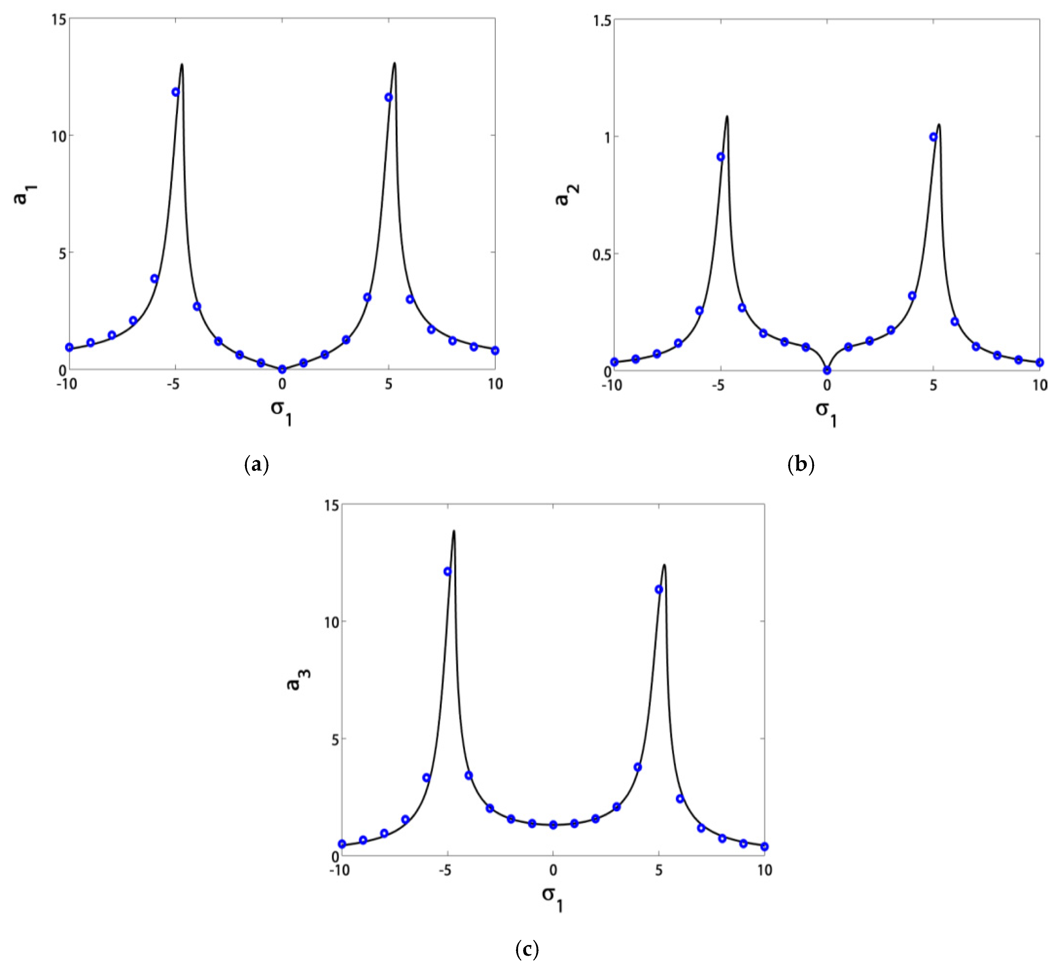
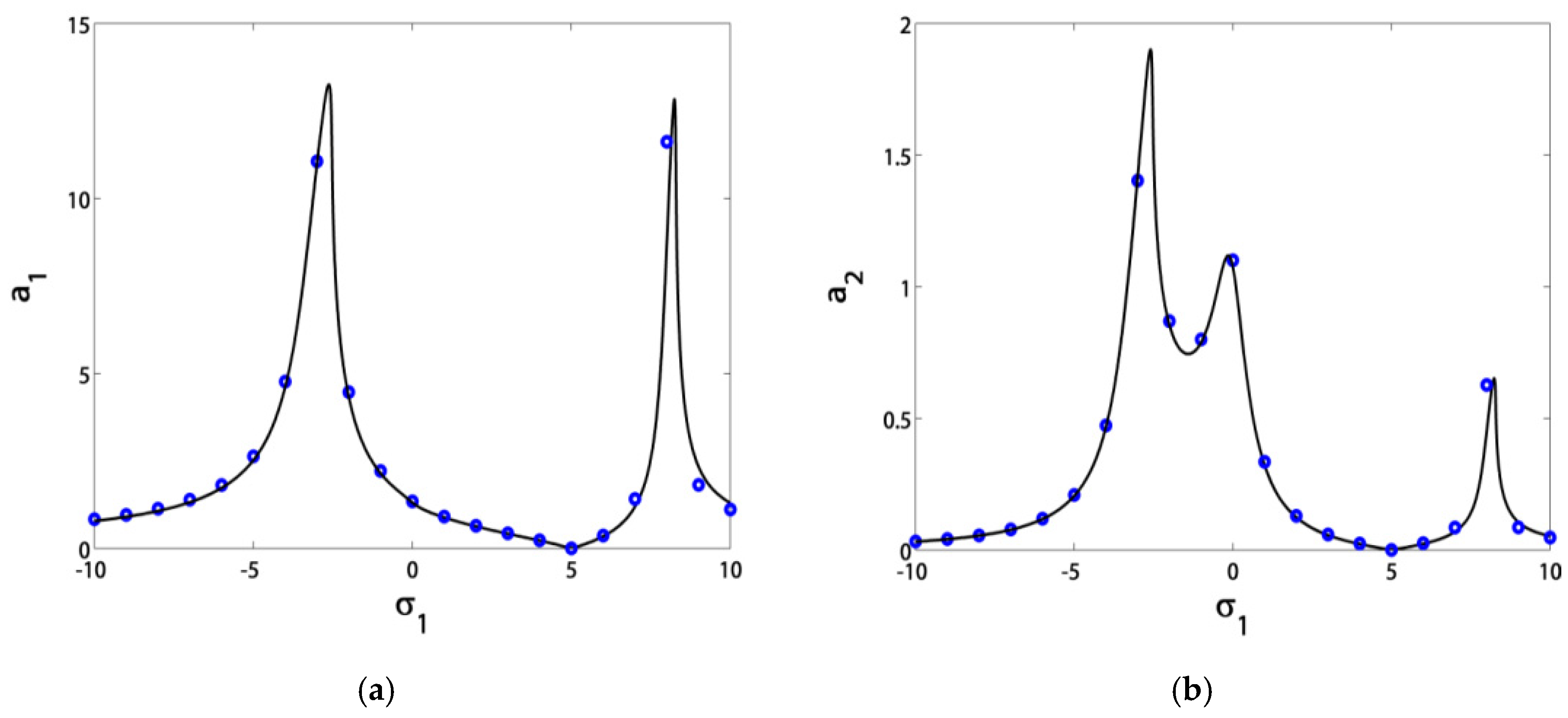
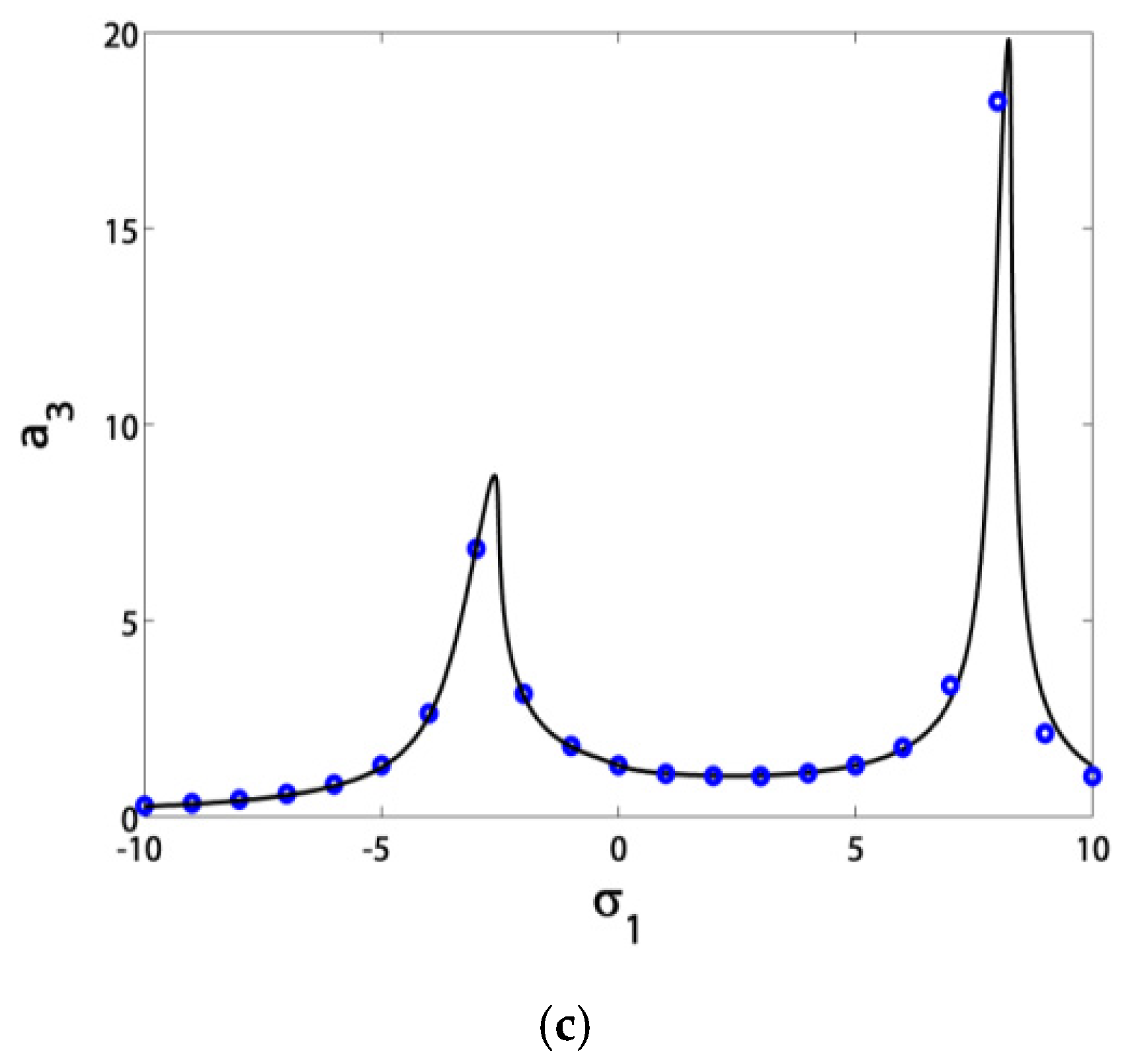
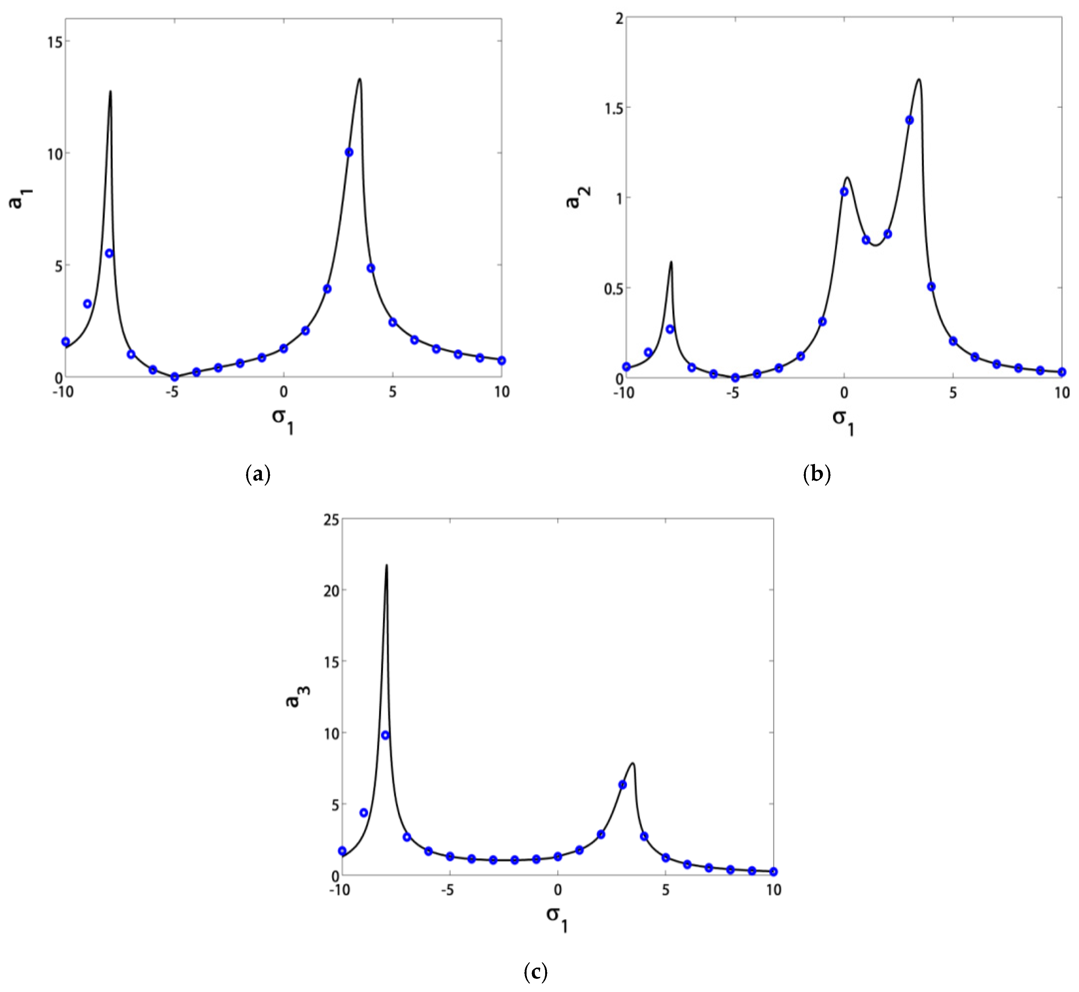
3.3. Validation Curves

This section shows the closeness between the analytical and numerical solutions in Figure 13, Figure 14, Figure 15, Figure 16, Figure 17, Figure 18 and Figure 19 for the responses shown above. These results confirm the validity of the proposed modeling and control strategy.

4. Conclusions

This work addressed the control of the rotating blade vibrations via MFC sensors and actuators by applying the PPF algorithm. An asymptotic analysis extracted the equations governing the nonlinear dynamics of the controlled blade. Several responses were included to portray the dynamical behavior of the blade under control. Moreover, an extensive comparison was fulfilled to show the closeness between the analytical and numerical results.
We can summarize the results as follows:
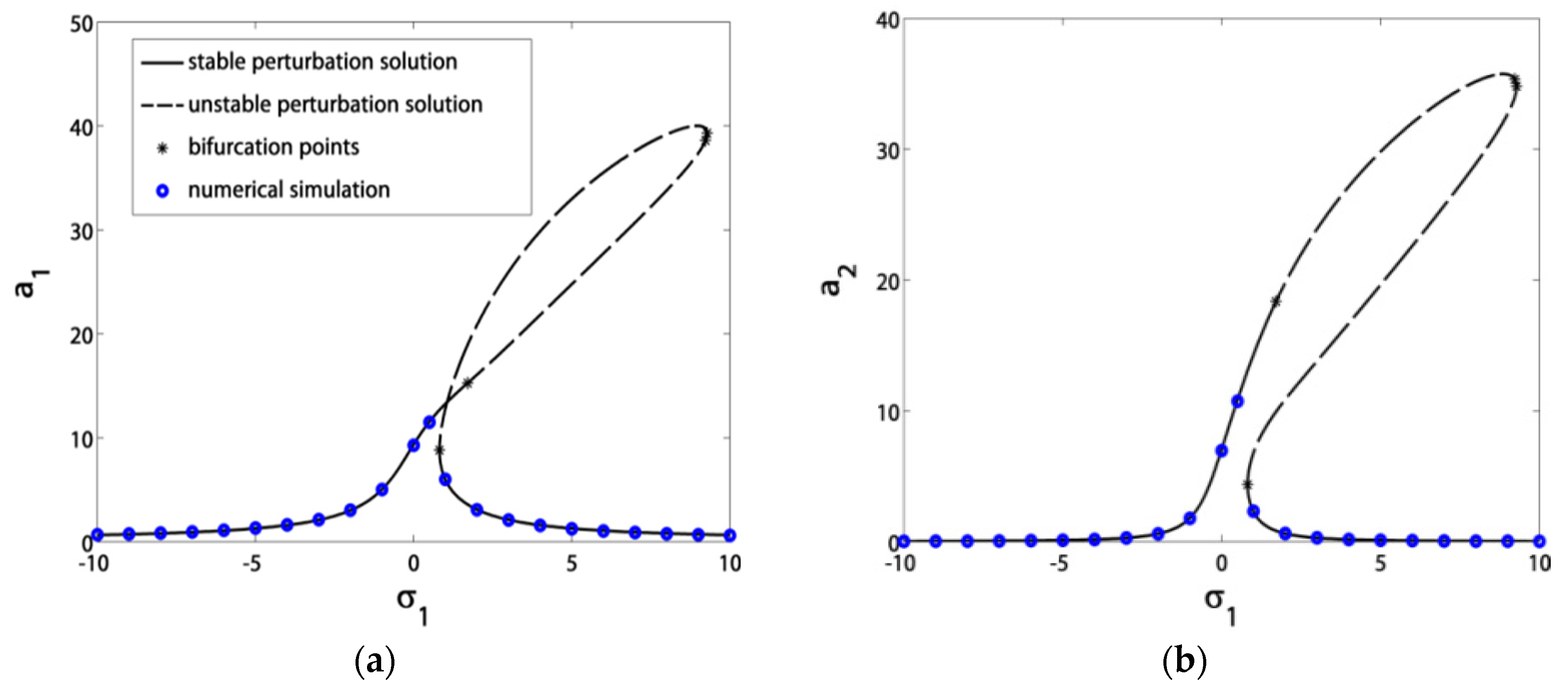
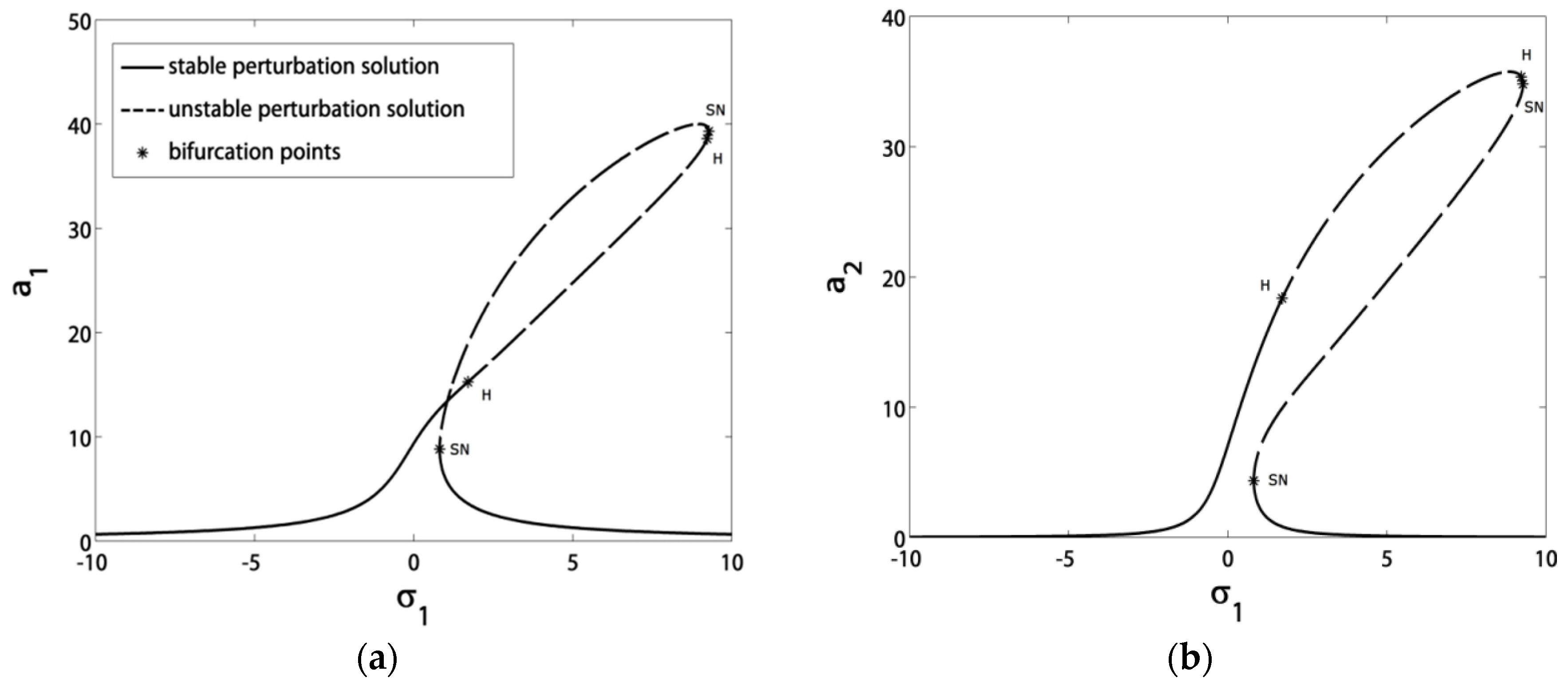
  • Before control, the blade suffered from severe vibrations and jumps due to the existence of bifurcation points. After control, the blade exhibited stable solutions without jumps due to the absence of bifurcation points;
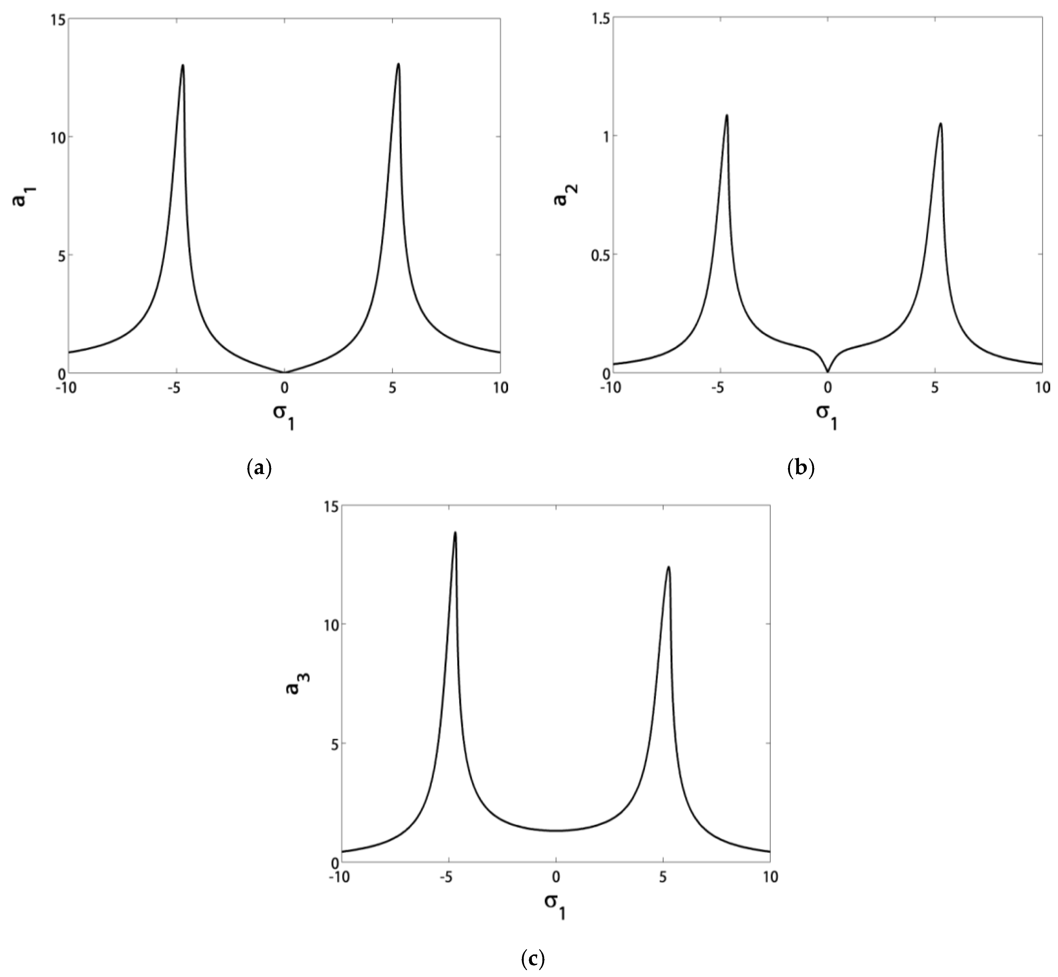
  • The blade vibrations reached minimum levels in the range of σ1 ∈ [−3, 3], especially at σ1 = 0;
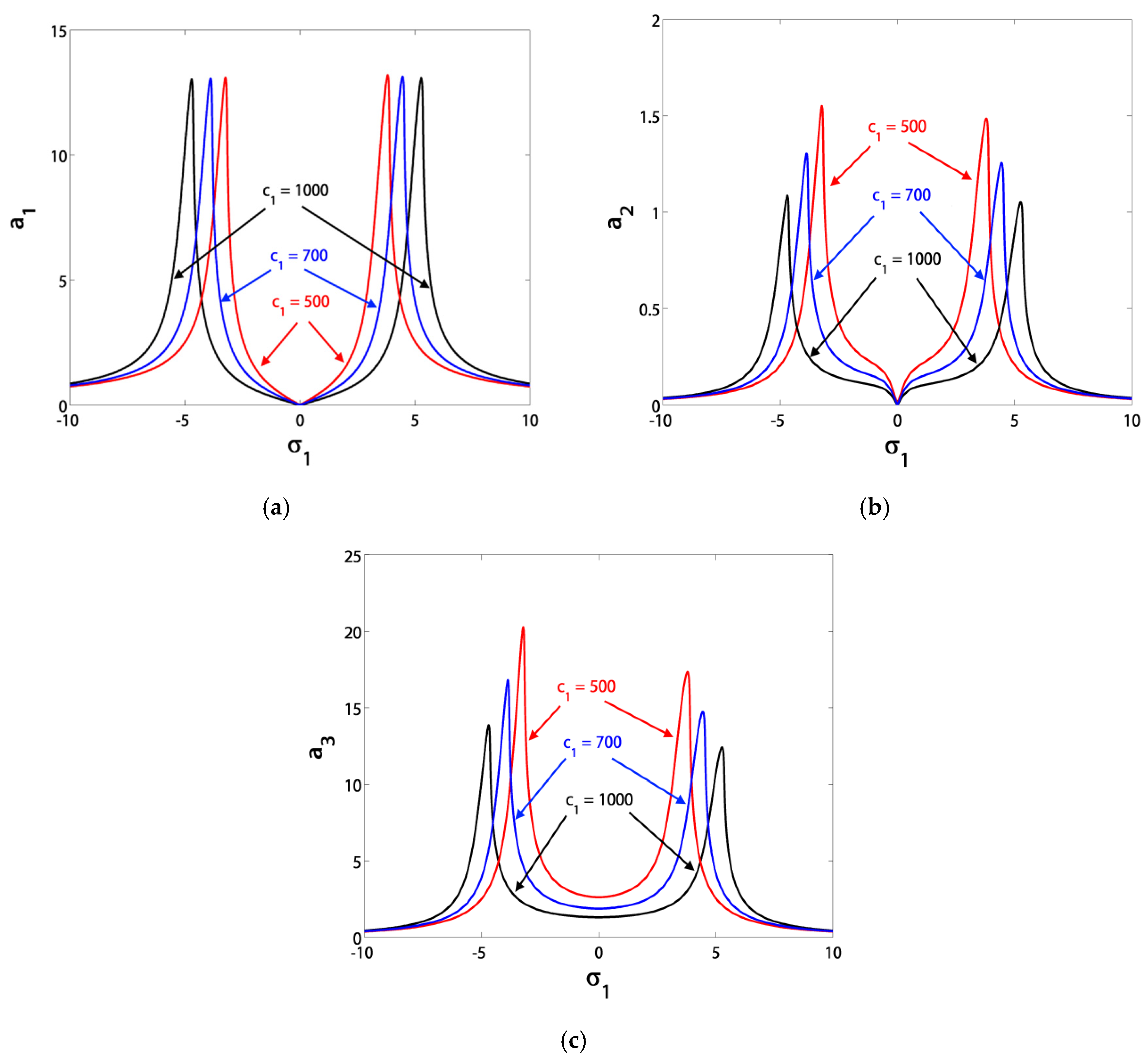
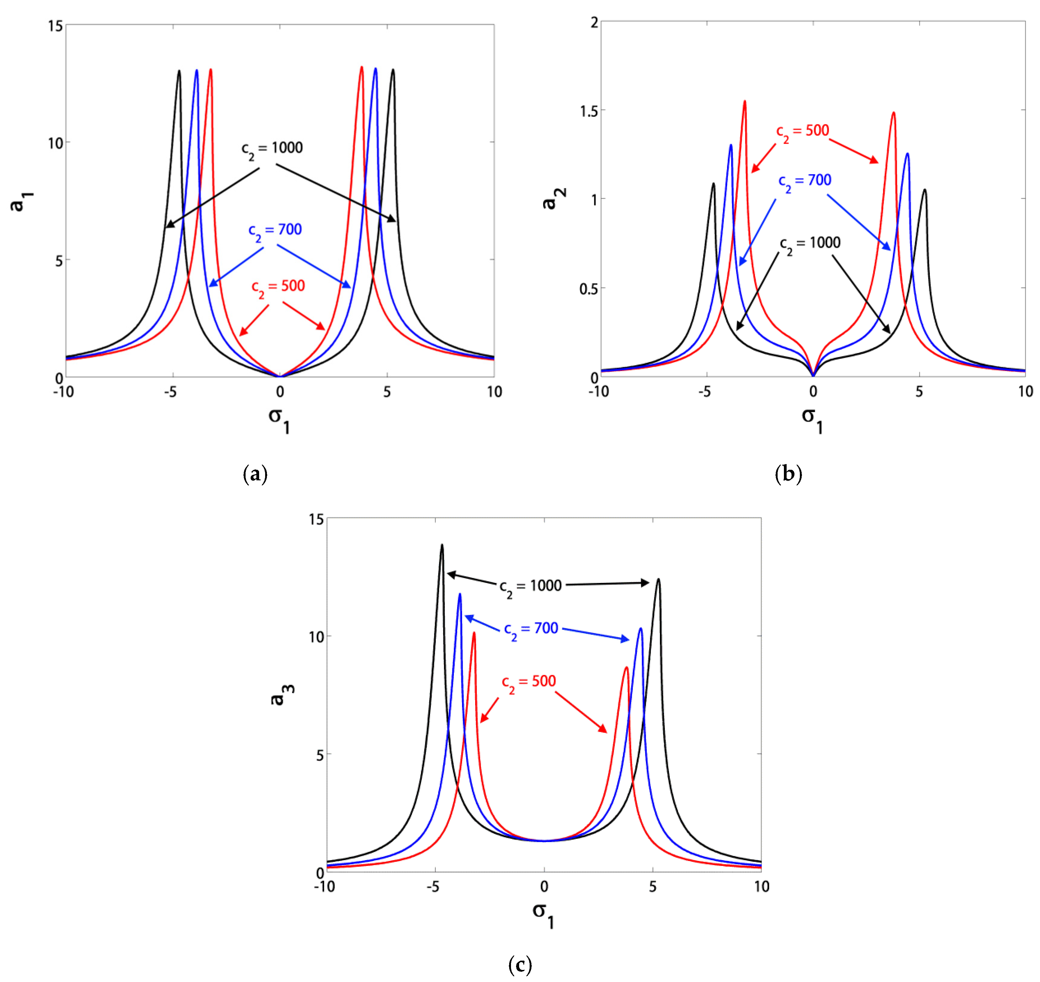
  • The minimum amplitude bandwidth could be adjusted via the control signal gain c1 or the feedback signal gain c2;
  • If we guaranteed that σ1 = σ2, then the blade operated safely in the range of σ1 ∈ [−5, 5];
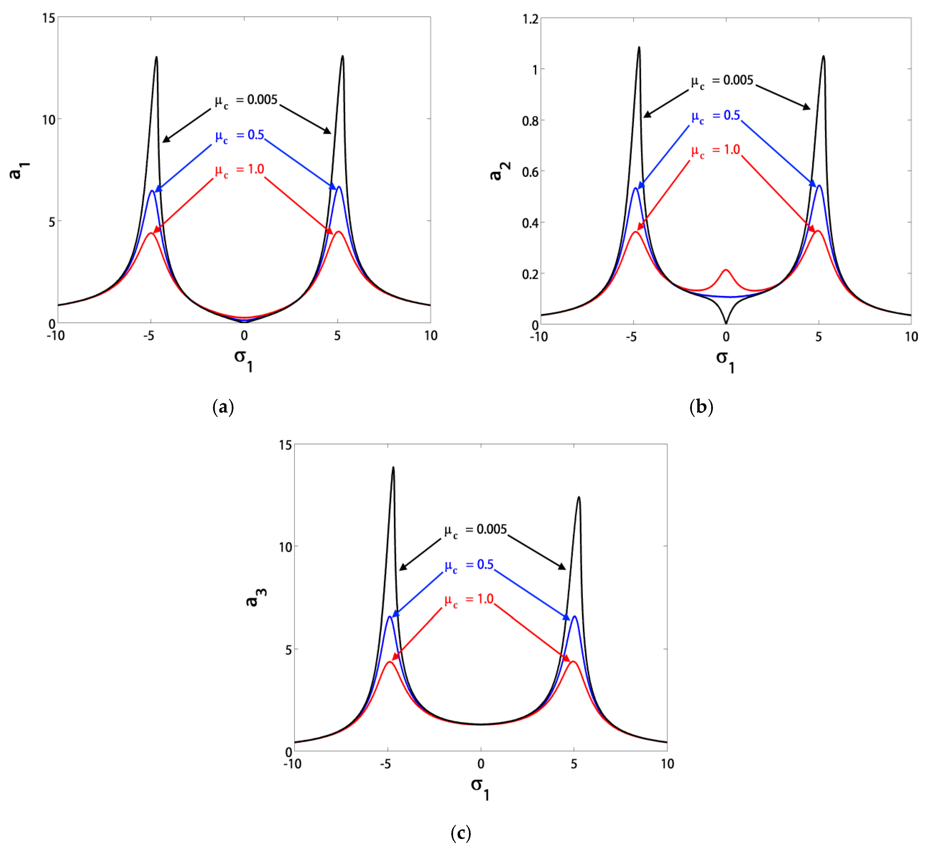
  • The controller damping μc was inversely proportional with the minimum vibratory level reached at σ1 = σ2;
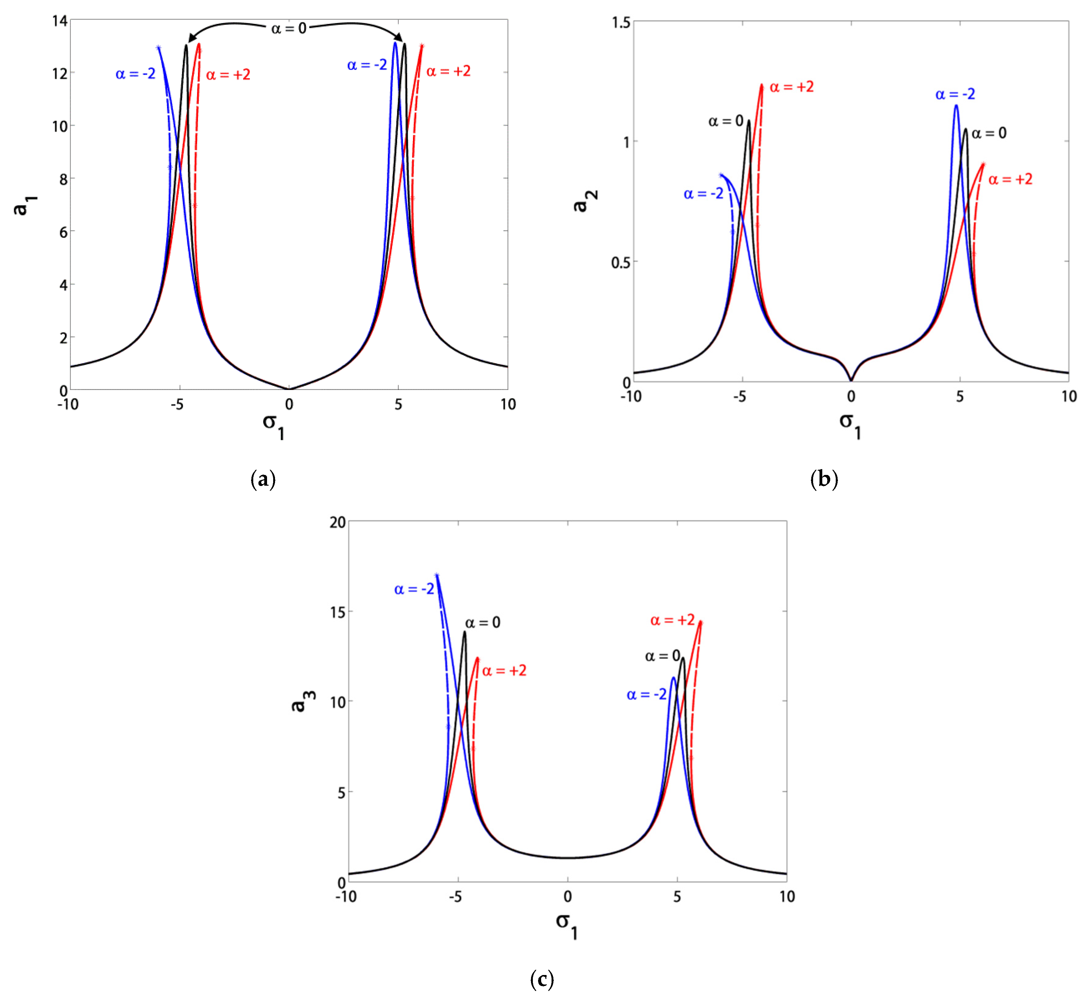
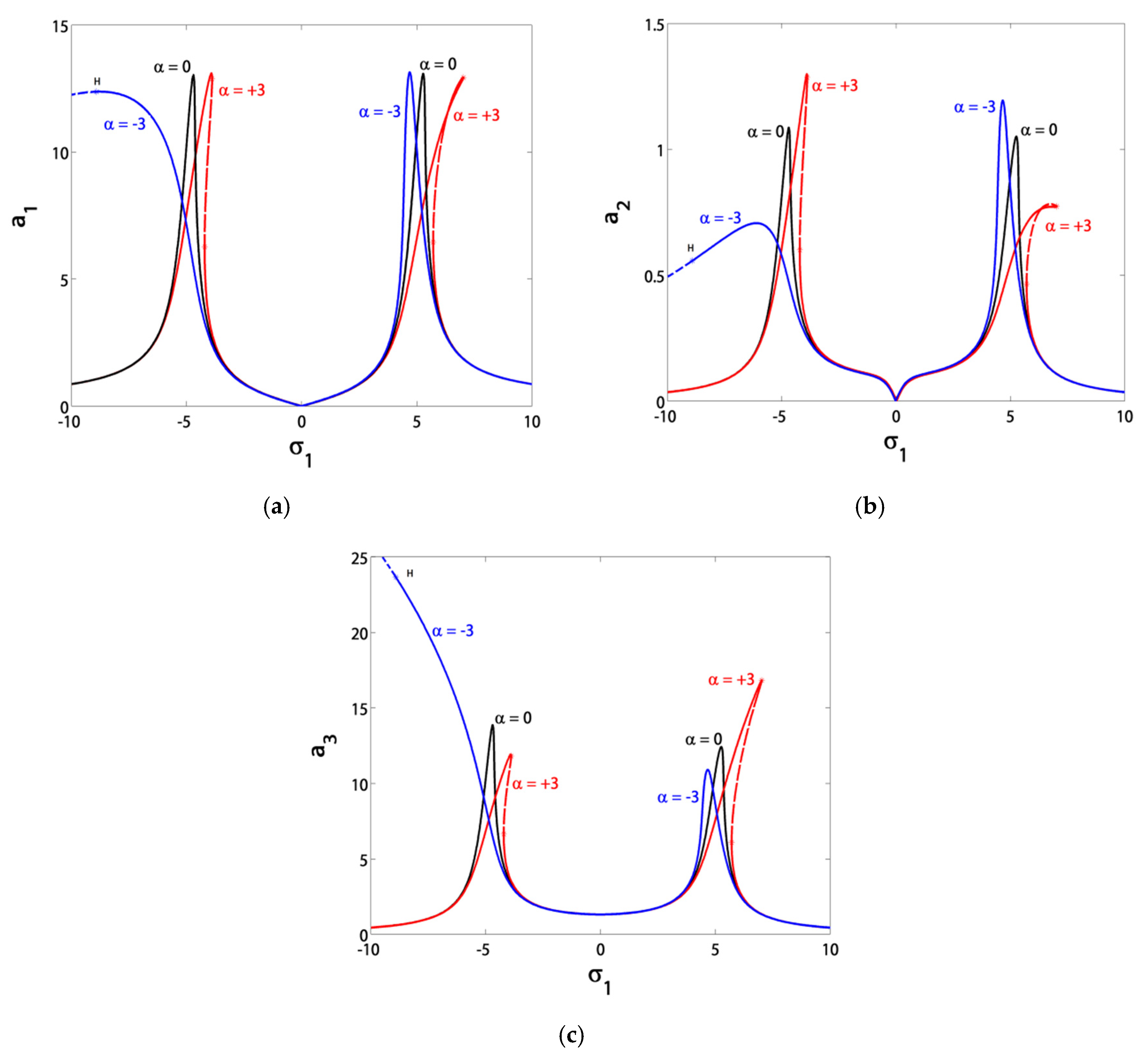
  • The controller nonlinearity parameter α should stay in the range of α ∈ (−3, 3), either for hardening or softening effects in the response curves without creating new jumps;
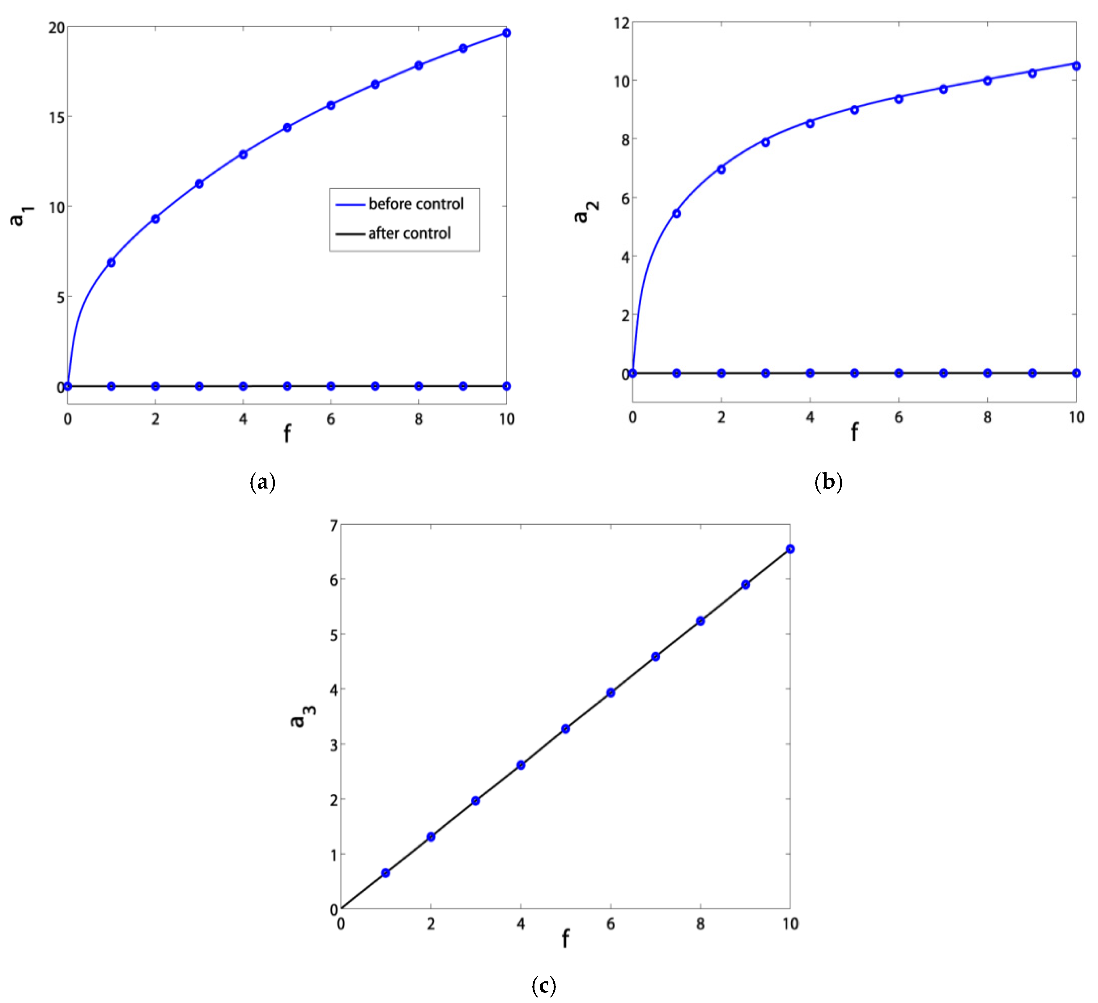
  • The blade vibration amplitudes were very sensitive to small rises in the excitation amplitude f before control. However, after control, they became saturated at a level of almost zero thanks to channeling most of the vibration energy to the controller.

Author Contributions

Y.S.H. and A.K. developed the idea of this research and made the problem formulation; Y.S.H. and A.K. derived the formulas, made the calculations, and performed the simulation study; Y.S.H., A.K., and J.T.M. oversaw all aspects of the research, data analysis, writing, and validation, prepared the initial draft of the paper, and revised this manuscript. All authors have read and agreed to the published version of the manuscript.

Funding

The authors received financial support from Taif University Researchers Supporting Project Number (TURSP-2020/155), Taif University, Taif, Saudi Arabia.

Acknowledgments

This research was supported by Taif University Researchers Supporting Project Number (TURSP-2020/155), Taif University, Taif, Saudi Arabia.

Conflicts of Interest

The authors declare that there is no conflict of interest.

Abbreviations

p, q, p, q, p, qHorizontal and vertical displacements, velocities, and accelerations of the blade’s cross-section.
y ¨ , y ˙ , y Acceleration, velocity, and displacement of the PPF controller.
μ , μ c Damping coefficients of the blade and controller.
ω , ω c Linear natural frequencies of the blade and controller.
β 11 , β 21 , β 13 , β 22 , β 5 Coupling factors between the blade’s vibrational directions.
β 5 , α Cubic nonlinearity coefficients of the blade and controller.
β 14 , β 24 Parametric excitation coefficients.
f 0 , f Amplitudes of the excitation force.
Ω ,   σ 1 , σ 2 Excitation frequency and detuning parameters.
c 1 , c 2 Gains of the control and feedback signals.

Appendix A

The considered thin-walled blade of length L and thickness h , shown in Figure A1, is connected to a rigid hub, which spun with an angular velocity Ω . A harmonic excitation F = f 0 + f cos ( Ω t ) may affect the blade’s rotation. Due to the blade’s flexural vibration, an angle γ appeared, and for twisting, another angle β = β 0 z / L appeared. A bunch of assumptions should be imposed to continue the analysis:
  • There will be no deformation in the cross-section for the long-term operation;
  • The blade’s thickness is very small, compared with its radius of gyration;
  • The blade can be considered an Euler–Bernoulli beam to neglect the shear force transversally;
  • In addition, we can neglect the elongation axially compared to the shown deflections.
Figure A1. Cross-section plane of the studied blade.
Symmetry 12 01984 g0a1
According to axes rotation rules, the rotary axes x p and y p could be related to the stationary axes x and y . The extended Hamilton principle was used for deriving the equations of motion. Considering K and U are the kinetic and strain energies, respectively, W is the virtual work due to external forces, and δ is the variation operator, we have
0 t ( δ K δ U + δ W ) d t = 0
In [12,13], detailed substitutions and extractions have been fulfilled to get the normalized equations of motion as
u ¨ 0 F 2 u 0 F 2 [ R ( z ) u 0 + R ( z ) u 0 ] + α Δ T u 0 [ α 3 ( z ) v 0 α 6 ( z ) u 0 ] = u 0 ( u 0 u 0 + v 0 v 0 ) + u 0 [ 1 2 ( u 0 ) 2 + 1 2 ( v 0 ) 2 ] F ˙ ( R 0 + z ) + p x
v ¨ 0 F 2 [ R ( z ) v 0 + R ( z ) v 0 ] + α Δ T v 0 [ α 3 ( z ) u 0 α 4 ( z ) v 0 ] = v 0 ( u 0 u 0 + v 0 v 0 ) + v 0 [ 1 2 ( u 0 ) 2 + 1 2 ( v 0 ) 2 ] + p y
The single-term Galerkin procedure is applied to Equation (A2) to represent the vibrational modes as
u 0 = G ( z )   p ( t )
v 0 = G ( z )   q ( t )
where p ( t ) , and   q ( t )   are the temporal deflections of the blade. The linear free undamped mode G ( z ) takes the form
G ( z ) = cosh ( Γ z ) cos ( Γ z ) [ cosh Γ + cos Γ sinh Γ + sin Γ ] [ sinh ( Γ z ) sin ( Γ z ) ]
where Γ is the solution of the equation cosh Γ cos Γ + 1 = 0 . Inserting Equations (A3) and (A4) into Equation (A2), then continuing with the Galerkin procedure and simplifying yields the system
p ¨ + 2 μ p ˙ + ω 2 p + β 13 q ˙ + β 11 q + β 5 p q 2 + β 5 p 3 = 2 f 0 f β 14 p cos ( Ω t ) + f 2 β 14 p   cos 2 ( Ω t )   + f β 16 Ω sin ( Ω t )
q ¨ + 2 μ q ˙ + ω 2 q + β 22 p ˙ + β 21 p + β 5 p 2 q + β 5 q 3 = 2 f 0 f β 24 q cos ( Ω t ) + f 2 β 24 q   cos 2 ( Ω t )
where all the parameters are given in detail in [12,13].

Appendix B

The elements r i j ( i , j = 1 , , 4 ) of the Jacobian matrix J given in Equation (14) are as follows:
r 11 = μ β 5 8 ω a 2 s 2 sin ( 2 ϕ 2 s ) + β 14 f 2 8 ω sin ( 2   ϕ 1 s )
r 12 = β 14 f 2 4 ω a 1 s cos ( 2   ϕ 1 s ) + β 16 Ω f 2 ω sin ϕ 1 s
r 13 = β 13 2 cos ϕ 2 s β 11 2 ω sin ϕ 2 s β 5 4 ω a 1 s a 2 s sin ( 2 ϕ 2 s )
r 14 = β 13 2 a 2 s sin ϕ 20 β 11 2 ω a 2 s cos ϕ 2 s β 5 4 ω a 1 s a 2 s 2 cos ( 2 ϕ 2 s )
r 15 = c 1 2 ω sin ϕ 3 s
r 16 = c 1 2 ω a 3 s cos ϕ 3 s
r 21 = β 13 2 a 2 s a 1 s 2 sin ϕ 2 s + β 11 2 ω a 2 s a 1 s 2 cos ϕ 2 s 3 β 5 4 ω a 1 s β 16 Ω f 2 ω 1 a 1 s 2 sin ϕ 1 s c 1 2 ω a 3 s a 1 s 2 cos ϕ 3 s
r 22 = β 14 f 2 4 ω sin ( 2 ϕ 1 s ) + β 16 Ω f 2 ω 1 a 1 s cos ϕ 1 s
r 23 = β 13 2 1 a 1 s sin ϕ 2 s β 11 2 ω 1 a 1 s cos ϕ 2 s β 5 2 ω a 2 s β 5 4 ω a 2 s cos ( 2 ϕ 2 s )
r 24 = β 13 2 a 2 s a 1 s cos ϕ 2 s + β 11 2 ω a 2 s a 1 s sin ϕ 2 s + β 5 4 ω a 2 s 2 sin ( 2 ϕ 2 s )
r 25 = c 1 2 ω 1 a 1 s cos ϕ 3 s
r 26 = c 1 2 ω a 3 s a 1 s sin ϕ 3 s
r 31 = β 22 2 cos ϕ 2 s + β 21 2 ω sin ϕ 2 s + β 5 4 ω a 1 s a 2 s sin ( 2 ϕ 2 s )
r 32 = β 24 f 2 4 ω a 2 s cos ( 2 ϕ 1 s 2 ϕ 2 s )
r 33 = μ + β 5 8 ω a 1 s 2 sin ( 2 ϕ 2 s ) + β 24 f 2 8 ω sin ( 2 ϕ 1 s 2 ϕ 2 s )
   r 34 = β 22 2 a 1 s sin ϕ 2 s + β 21 2 ω a 1 s cos ϕ 2 s + β 5 4 ω a 1 s 2 a 2 s cos ( 2 ϕ 2 s ) β 24 f 2 4 ω a 2 s cos ( 2 ϕ 1 s 2 ϕ 2 s )
r 35 = r 36 = 0
r 41 = β 22 2 1 a 2 s sin ϕ 2 s + β 21 2 ω 1 a 2 s cos ϕ 2 s + β 5 2 ω   a 1 s + β 5 4 ω a 1 s cos ( 2 ϕ 2 s ) 3 β 5 4 ω a 1 s β 13 2 a 2 s a 1 s 2 sin ϕ 2 s + β 11 2 ω a 2 s a 1 s 2 cos ϕ 2 s β 16 Ω f 2 ω 1 a 1 s 2 sin ϕ 1 s c 1 2 ω a 3 s a 1 s 2 cos ϕ 3 s
r 42 = β 24 f 2 4 ω sin ( 2 ϕ 1 s 2 ϕ 2 s ) β 14 f 2 4 ω sin ( 2 ϕ 1 s ) + β 16 Ω f 2 ω 1 a 1 s cos ϕ 1 s
r 43 = β 22 2 a 1 s a 2 s 2 sin ϕ 2 s β 21 2 ω a 1 s a 2 s 2 cos ϕ 2 s β 5 2 ω a 2 s β 5 4 ω a 2 s cos ( 2 ϕ 2 s ) + 3 β 5 4 ω a 2 s + β 13 2 1 a 1 s sin ϕ 2 s β 11 2 ω 1 a 1 s cos ϕ 2 s
r 44 = β 22 2 a 1 s a 2 s cos ϕ 2 s β 21 2 ω a 1 s a 2 s sin ϕ 2 s β 5 4 ω a 1 s 2 sin ( 2 ϕ 2 s ) β 24 f 2 4 ω sin ( 2 ϕ 1 s 2 ϕ 2 s ) + β 13 2 a 2 s a 1 s cos ϕ 2 s + β 11 2 ω a 2 s a 1 s sin ϕ 2 s + β 5 4 ω a 2 s 2 sin ( 2 ϕ 2 s )
r 45 = c 1 2 ω 1 a 1 s cos ϕ 3 s
r 46 = c 1 2 ω a 3 s a 1 s sin ϕ 3 s
r 51 = c 2 2 ω c sin ϕ 3 s
r 52 = r 53 = r 54 = 0
r 55 = μ c
r 56 = c 2 2 ω c a 1 s cos ϕ 3 s
r 61 = c 2 2 ω c 1 a 3 s cos ϕ 3 s β 13 2 a 2 s a 1 s 2 sin ϕ 2 s + β 11 2 ω a 2 s a 1 s 2 cos ϕ 2 s 3 β 5 4 ω a 1 s β 16 Ω f 2 ω 1 a 1 s 2 sin ϕ 1 s c 1 2 ω a 3 s a 1 s 2 cos ϕ 3 s
r 62 = β 14 f 2 4 ω sin ( 2 ϕ 1 s ) + β 16 Ω f 2 ω 1 a 1 s cos ϕ 1 s
r 63 = β 13 2 1 a 1 s sin ϕ 2 s β 11 2 ω 1 a 1 s cos ϕ 2 s β 5 2 ω a 2 s β 5 4 ω a 2 s cos ( 2 ϕ 2 s )
r 64 = β 13 2 a 2 s a 1 s cos ϕ 2 s + β 11 2 ω a 2 s a 1 s sin ϕ 2 s + β 5 4 ω a 2 s 2 sin ( 2 ϕ 2 s )
r 65 = 3 α 4 ω c a 3 s + c 2 2 ω c a 1 s a 3 s 2 cos ϕ 3 s + c 1 2 ω 1 a 1 s cos ϕ 3 s
r 66 = c 2 2 ω c a 1 s a 3 s sin ϕ 3 s c 1 2 ω a 3 s a 1 s sin ϕ 3 s
The elements of the stability criteria given in Equation (16) are as follows:
γ 1 = i = 1 6 r i i
γ 2 = 1 2 ! i = 1 6 j = 1 6 r i i r j j r i j r j i
γ 3 = 1 3 ! i = 1 6 j = 1 6 k = 1 6 r i i r j j r k k 3 r i i r j k r k j + 2 r i j r j k r k i
γ 4 = 1 4 ! i = 1 6 j = 1 6 k = 1 6 l = 1 6 r i i r j j r k k r l l 6 r i i r j j r k l r l k + 8 r i i r j k r k l r l j + 3 r i j r j i r k l r l k 6 r i j r j k r k l r l i
γ 5 = 1 5 ! i = 1 6 j = 1 6 k = 1 6 l = 1 6 m = 1 6 ( r i i r j j r k k r l l r m m 10 r i i r j j r k k r l m r m l + 20 r i i r j j r k l r l m r m k 20 r i j r j i r k l r l m r m k + 15 r i i r j k r k j r l m r m l 30 r i i r j k r k l r l m r m j + 24 r i j r j k r k l r l m r m i )
γ 6 = 1 6 ! i = 1 6 j = 1 6 k = 1 6 l = 1 6 m = 1 6 n = 1 6 ( r i i r j j r k k r l l r m m r n n 15 r i i r j j r k k r l l r m n r n m + 40 r i i r j j r k k r l m r m n r n l 90 r i i r j j r k l r l m r m n r n k + 144 r i i r j k r k l r l m r m n r n j + 45 r i i r j j r k l r l k r m n r n m 15 r i j r j i r k l r l k r m n r n m 120 r i j r j k r k l r l m r m n r n i   + 40 r i j r j k r k i r l m r m n r n l + 90 r i j r j i r k l r l m r m n r n k 120 r i i r j k r k j r l m r m n r n l )

References

  1. Yoo, H.H.; Kwak, J.Y.; Chung, J. Vibration analysis of rotating pre-twisted blades with a concentrated mass. J. Sound Vib. 2001, 240, 891–908. [Google Scholar] [CrossRef]
  2. Lin, C.Y.; Chen, L.W. Dynamic stability of rotating pre-twisted blades with a constrained damping layer. Compos. Struct. 2003, 61, 235–245. [Google Scholar] [CrossRef]
  3. Oh, S.Y.; Song, O.; Librescu, L. Effects of pretwist and presetting on coupled bending vibrations of rotating thin-walled composite beams. Int. J. Solids Struct. 2003, 40, 1203–1224. [Google Scholar] [CrossRef]
  4. Librescu, L.; Oh, S.Y.; Song, O. Spinning thin-walled beams made of functionally graded materials: Modeling, vibration and instability. Eur. J. Mech. A Solids 2004, 23, 499–515. [Google Scholar] [CrossRef]
  5. Sinha, S.K. Dynamic characteristics of a flexible bladed-rotor with Coulomb damping due to tip-rub. J. Sound Vib. 2004, 273, 875–919. [Google Scholar] [CrossRef]
  6. Hamdan, M.N.; El-Sinawi, A.H. On the non-linear vibrations of an inextensible rotating arm with setting angle and flexible hub. J. Sound Vib. 2005, 281, 375–398. [Google Scholar] [CrossRef]
  7. Choi, S.C.; Park, J.S.; Kim, J.H. Active damping of rotating composite thin-walled beams using MFC actuators and PVDF sensors. Compos. Struct. 2006, 76, 362–374. [Google Scholar] [CrossRef]
  8. Choi, S.C.; Park, J.S.; Kim, J.H. Vibration control of pre-twisted rotating composite thin-walled beams with piezoelectric fiber composites. J. Sound Vib. 2007, 300, 176–196. [Google Scholar] [CrossRef]
  9. Fazelzadeh, S.A.; Malekzadeh, P.; Zahedinejad, P.; Hosseini, M. Vibration analysis of functionally graded thin-walled rotating blades under high temperature supersonic flow using the differential quadrature method. J. Sound Vib. 2007, 306, 333–348. [Google Scholar] [CrossRef]
  10. Vadiraja, D.N.; Sahasrabudhe, A.D. Vibration analysis and optimal control of rotating pre-twisted thin-walled beams using MFC actuators and sensors. Thin-Walled Struct. 2009, 47, 555–567. [Google Scholar] [CrossRef]
  11. Younesian, D.; Esmailzadeh, E. Vibration suppression of rotating beams using time-varying internal tensile force. J. Sound Vib. 2011, 330, 308–320. [Google Scholar] [CrossRef]
  12. Yao, M.H.; Chen, Y.P.; Zhang, W. Nonlinear vibrations of blade with varying rotating speed. Nonlinear Dyn. 2012, 68, 487–504. [Google Scholar] [CrossRef]
  13. Yao, M.H.; Zhang, W.; Chen, Y.P. Analysis on nonlinear oscillations and resonant responses of a compressor blade. Acta Mech. 2014, 225, 3483–3510. [Google Scholar] [CrossRef]
  14. Latalski, J.; Warminski, J.; Rega, G. Bending-twisting vibrations of a rotating hub-thin-walled composite beam system. Math. Mech. Solids 2017, 22, 1303–1325. [Google Scholar] [CrossRef]
  15. Rafiee, M.; Nitzsche, F.; Labrosse, M. Dynamics, vibration and control of rotating composite beams and blades: A critical review. Thin-Walled Struct. 2017, 119, 795–819. [Google Scholar] [CrossRef]
  16. Chen, J.; Li, Q.S. Vibration characteristics of a rotating pre-twisted composite laminated blade. Compos. Struct. 2019, 208, 78–90. [Google Scholar] [CrossRef]
  17. Liu, T.R.; Gong, A.L. Theoretical modeling and vibration control for pre-twisted composite blade based on LLI controller. Trans. Inst. Meas. Control. 2020, 42, 1255–1270. [Google Scholar] [CrossRef]
  18. Zhang, Y.F.; Niu, Y.; Zhang, W. Nonlinear vibrations and internal resonance of pretwisted rotating cantilever rectangular plate with varying cross-section and aerodynamic force. Eng. Struct. 2020, 225, 111259. [Google Scholar] [CrossRef]
  19. Zhang, W.; Liu, G.; Siriguleng, B. Saturation phenomena and nonlinear resonances of rotating pretwisted laminated composite blade under subsonic air flow excitation. J. Sound Vib. 2020, 478, 115353. [Google Scholar] [CrossRef]
  20. Zhang, W.; Niu, Y.; Behdinan, K. Vibration characteristics of rotating pretwisted composite tapered blade with graphene coating layers. Aerosp. Sci. Technol. 2020, 98, 105644. [Google Scholar] [CrossRef]
  21. Wang, Z.; Almeida, J.H.S.; St-Pierre, L.; Wang, Z.; Castro, S.G.P. Reliability-based buckling optimization with an accelerated Kriging metamodel for filament-wound variable angle tow composite cylinders. Compos. Struct. 2020, 254. [Google Scholar] [CrossRef]
  22. Almeida, J.H.S.; Bittrich, L.; Spickenheuer, A. Improving the open-hole tension characteristics with variable-axial composite laminates: Optimization, progressive damage modeling and experimental observations. Compos. Sci. Technol. 2020, 185. [Google Scholar] [CrossRef]
  23. Monticeli, F.M.; Almeida, J.H.S.; Neves, R.M.; Ornaghi, F.G.; Ornaghi, H.L. On the 3D void formation of hybrid carbon/glass fiber composite laminates: A statistical approach. Compos. Part A Appl. Sci. Manuf. 2020, 137, 106036. [Google Scholar] [CrossRef]
  24. Shin, C.; Hong, C.; Jeong, W.B. Active vibration control of clamped beams using positive position feedback controllers with moment pair. J. Mech. Sci. Technol. 2012, 26, 731–740. [Google Scholar] [CrossRef]
  25. El-Ganaini, W.A.; Saeed, N.A.; Eissa, M. Positive position feedback (PPF) controller for suppression of nonlinear system vibration. Nonlinear Dyn. 2013, 72, 517–537. [Google Scholar] [CrossRef]
  26. El-Ganaini, W.A.; Kandil, A.; Eissa, M.; Kamel, M. Effects of delayed time active controller on the vibration of a nonlinear magnetic levitation system to multi excitations. J. Vib. Control. 2016, 22, 1257–1275. [Google Scholar] [CrossRef]
  27. Hamed, Y.S.; El Shehry, A.; Sayed, M. Nonlinear modified positive position feedback control of cantilever beam system carrying an intermediate lumped mass. Alex. Eng. J. 2020, 59, 3847–3862. [Google Scholar] [CrossRef]
  28. Nayfeh, A.H.; Mook, D.T. Nonlinear Oscillations; Wiley: New York, NY, USA, 1995. [Google Scholar] [CrossRef]
Figure 1. Process of controlling the rotating blade via macro fiber composite (MFC).
Symmetry 12 01984 g001
Figure 2. The blade’s horizontal and vertical amplitude responses to the excitation frequency detuning σ 1 before control: (a) horizontal, (b) vertical.
Symmetry 12 01984 g002
Figure 3. The blade and controller amplitude responses to the excitation frequency detuning σ 1 after control: (a) horizontal, (b) vertical, (c) controller.
Symmetry 12 01984 g003
Figure 4. Effect of the control signal gain c 1 on the blade and the controller amplitude responses to the excitation frequency detuning σ 1 : (a) horizontal, (b) vertical, (c) controller.
Symmetry 12 01984 g004
Figure 5. Effect of the feedback signal gain c 2 on the blade and the controller amplitude responses to the excitation frequency detuning σ 1 : (a) horizontal, (b) vertical, (c) controller.
Symmetry 12 01984 g005
Figure 6. Effect of the controller damping μ c on the blade and the controller amplitude responses to the excitation frequency detuning σ 1 : (a) horizontal, (b) vertical, (c) controller.
Symmetry 12 01984 g006
Figure 7. Effect of the controller frequency detuning σ 2 on the blade and the controller amplitude responses to the excitation frequency detuning σ 1 : (a) horizontal, (b) vertical, (c) controller.
Symmetry 12 01984 g007
Figure 8. Effect of the controller nonlinearity parameter α on the blade and the controller amplitude responses to the excitation frequency detuning σ 1 for α = { 2 ,   0 ,   + 2 } : (a) horizontal, (b) vertical, (c) controller.
Symmetry 12 01984 g008
Figure 9. Effect of the controller nonlinearity parameter α on the blade and the controller amplitude responses to the excitation frequency detuning σ 1 for α = { 3 ,   0 ,   + 3 } : (a) horizontal, (b) vertical, (c) controller.
Symmetry 12 01984 g009
Figure 10. The blade’s horizontal and vertical amplitude responses to the excitation amplitude f before and after control at σ 1 = σ 2 = 0 : (a) horizontal, (b) vertical, (c) controller.
Symmetry 12 01984 g010
Figure 11. The blade’s horizontal and vertical temporal displacements before control: (a) horizontal, (b) vertical.
Symmetry 12 01984 g011
Figure 12. The blade’s horizontal and vertical, as well as the controller’s, temporal displacements after control: (a) horizontal, (b) vertical, (c) controller.
Symmetry 12 01984 g012
Figure 13. The analytical and numerical blade’s amplitude, compared to the excitation frequency detuning σ 1 before control: (a) horizontal, (b) vertical.
Symmetry 12 01984 g013
Figure 14. The analytical and numerical blade’s amplitudes, compared to the excitation frequency detuning σ 1 after control at σ 2 = 0 : (a) horizontal, (b) vertical, (c) controller.
Symmetry 12 01984 g014
Figure 15. The analytical and numerical blade and controller amplitudes, compared to the excitation amplitude f before and after control: (a) horizontal, (b) vertical, (c) controller.
Symmetry 12 01984 g015
Figure 16. The analytical and numerical blade and controller amplitudes, compared to the excitation frequency detuning σ 1 after control at σ 2 = 5 : (a) horizontal, (b) vertical, (c) controller.
Symmetry 12 01984 g016aSymmetry 12 01984 g016b
Figure 17. The analytical and numerical blade and controller amplitudes, compared to the excitation frequency detuning σ 1 after control at σ 2 = 5 : (a) horizontal, (b) vertical, (c) controller.
Symmetry 12 01984 g017
Figure 18. The analytical and numerical blade’s amplitude, compared to the temporal displacements before control: (a) horizontal, (b) vertical.
Symmetry 12 01984 g018
Figure 19. The analytical and numerical blade and controller amplitudes, compared to the temporal displacements after control: (a) horizontal, (b) vertical, (c) controller.
Symmetry 12 01984 g019
Publisher’s Note: MDPI stays neutral with regard to jurisdictional claims in published maps and institutional affiliations.

