Multivariate Control Chart Based on Kernel PCA for Monitoring Mixed Variable and Attribute Quality Characteristics

Abstract

The need for a control chart that can visualize and recognize the symmetric or asymmetric pattern of the monitoring process with more than one type of quality characteristic is a necessity in the era of Industry 4.0. In the past, the control charts were only developed to monitor one kind of quality characteristic. Several control charts were created to deal with this problem. However, there are some problems and drawbacks to the conventional mixed charts. In this study, another approach is used to monitor mixed quality characteristics by applying the Kernel Principal Component Analyisis (KPCA) method. Using the Hotelling’s T² statistic, the kernel PCA mix chart is proposed to simultaneously monitor the variable and attribute quality characteristics. Due to its ability to estimate the asymmetric pattern of the mixed process, the kernel density estimation (KDE) used in the proposed chart has successfully estimated the control limits that produce ARL₀ at about 370 for $\alpha =0.00273$. Through several experiments based on the proportion of the attribute characteristics and kernel functions, the proposed chart demonstrates better performance in detecting outlier and shift in the process. When it is applied to monitor the synthetic data, the proposed chart can detect the shift accurately. Additionally, the proposed chart outperforms the performance of the conventional mixed chart based on PCA mix by producing lower false alarm with more accurate detection of out of control processes.

1. Introduction

The control chart can visualize the quality characteristics in a graphical form and calculate its control limit based on the symmetric or asymmetric distribution of the monitored processes. In statistical process control (SPC), two types of control chart have been developed based on the monitored quality characteristics, namely the variable and attribute charts [1]. The variable control chart is developed to monitor the metric quality characteristics (variable or ratio scale) such as length or height. On the other hand, to monitor the nonmetric quality characteristics (categorical scale), the attribute chart is used. Some works have developed the variable and attribute charts, especially to monitor more than one characteristic (multivariable or multiattribute characteristics). The Shewhart, multivariate exponentially weighted moving average (MEWMA), and multivariate cumulative sum (MCUSUM) type charts are developed to accommodate the multivariable characteristics [1].

The recent development of the Shewhart type chart includes the T²-PCA chart [2], the robust T² chart [3,4], the variable parameters (VP)-T² Hotelling chart [5], and the T² chart for short-run production [6]. Meanwhile, the latest development of MEWMA and MCUSUM charts covers an adaptive MEWMA chart [7], one-sided and two one-sided MEWMA charts [8], dual MCUSUM chart [9], Max MCUSUM for autocorrelated data [10], as well as the mixed multivariate memory control charts [11]. Other recent charts of the multiattribute charts consist of multiple dependent state repetitive sampling (MDSRS) [12] and fuzzy bivariate chart [13] for Poisson distribution, as well as the multinomial generalized likelihood ratio (MGLR) control chart for multinomial distribution [14].

To improve the product quality, the mixed monitoring procedure is necessary in the production process [15]. The quality characteristics in a product not only can be measured by the variable or attribute separately but also can be measured together using the mixed scheme. Therefore, to accommodate these needs, some researchers have developed the mixed characteristics charts. Aslam et al. [16] suggested the mixed chart by applying combined $\overline{X}$ and np charts in monitoring the quality processes. This mixed chart is developed by transforming the variable characteristics into attributes which are then monitored simultaneously on a chart. The performance of the mixed chart of Aslam et al. [16] was compared with hybrid exponential weighted moving average (HEWMA) in [17]. Wang et al. [18] proposed a spatial-sign covariance matrix-based chart by integrating the standardized ranks and spatial signs to calculate the mixed statistics. Finally, the T² based principal component analysis (PCA) mix chart is proposed to monitor the mixed characteristics processes [19] and to detect outlier [20] using the kernel-based control limit [21].

The drawback of the PCA mix chart was discovered when it was applied to inspect the extreme imbalanced categorical data or attribute characteristics. Ahsan et al. [19] found that the performance of PCA mix chart is decreased for an extremely imbalanced proportion of the attribute characteristics. Commonly, in the manufacturing process there is 95% good product and 5% defect product. To solve such issue, the kernel PCA (KPCA) method proposed by Schölkopf [22] can be employed to accommodate the difference in data type. KPCA is a nonlinear version of the conventional PCA that can model data from non-Gaussian distributions [23]. This approach can efficiently calculate principal component scores (PCs) on the high dimensional feature space using kernel functions [24]. This method is also applied in control chart and success in detecting outlier [25].

Based on the above considerations, this paper proposes a mixed multivariate control chart based on the KPCA method that can accommodate the different types of quality characteristics, named KPCA mix chart. In this approach, the attribute characteristics or the categorical data will be transformed into the dummy variables (numeric variables that reflect categorical data or attribute characteristics symbolized in 0 and 1). Further, along with the variable characteristics of the continuous data, the kernel matrix is formed, and the PCs from the mixed characteristics are computed. The computed PCs are then transformed into T² statistics. In estimating the control limit of T² statistics, this study uses kernel density estimation (KDE), the same approach used in Ahsan et al. [19] to find the asymmetric or even unknown pattern of the mixed characteristics. Moreover, to show the appropriateness of the proposed chart, its performance is compared with the PCA mix chart. The rest of the paper is organized as follows: Section 2 describes the proposed KPCA mix. The KDE control limit from the different kinds of kernel function are tabulated in Section 3. Section 4 presents the performance of the proposed chart in detecting outlier and shift in the process. The utilization of the proposed chart in simulated and real data is shown in Section 5. The managerial implication is described in Section 6. The conclusions and possible development of this paper are laid down in Section 7.

2. Kernel PCA Mix Control Chart

2.1. Kernel PCA

PCA is the basis of transformation to diagonalize the estimated covariance matrix C from input data $x_j,j=1,\dots .,n,x_j\in {ℝ}^p,{\displaystyle \sum _{j=1}^n{x}_j=0}$ defined as follows:

$$C=\frac{1}{n}{\displaystyle \sum _{j=1}^n{x}_j{x}_j^T}.$$

(1)

The new coordinate, principal component, is calculated based on the eigenvector projection of the input data. PCA works under the assumption that the data has a linear relationship. However, in the complex case such as the chemical industry or biology, the relationship of the data is not always linear. As a consequence, the conventional PCA has a poor performance for such a case [26].

To overcome the nonlinearity problem, Schölkopf et al. [22] introduced the kernel PCA method. The basic idea of this method is calculating the PCs in feature space by conducting a nonlinear mapping $\mathsf{\Phi }:{ℝ}^p\to F, x\mapsto X$ (see Figure 1). This can be done by involving kernel functions known from SVM [27]. In other words, PCA can be executed in feature space F by employing the kernel function.

Assume that the centered input data are mapped to feature space F, $\mathsf{\Phi }(x_1),\dots ,\mathsf{\Phi }(x_n)$. The covariance matrix in feature space can be written as:

$$C^F=\frac{1}{n}{\displaystyle \sum _{j=1}^n\mathsf{\Phi }(x_j)\mathsf{\Phi }{(x_j^{})}^T}.$$

(2)

The next step is finding the eigenvalues $\lambda \ge 0$ eigenvector $V\in F\backslash \left\{0\right\}$ that satisfies:

$$\lambda V=C^{F}V.$$

(3)

By substituting the $C^F$ in Equations (2) and (3), it can be found that:

$$\begin{array}{ll}\lambda V& =\left(\frac{1}{n}{\displaystyle \sum _{j=1}^n\mathsf{\Phi }(x_j)\mathsf{\Phi }{(x_j^{})}^T}\right)V\\ & =\frac{1}{n}{\displaystyle \sum _{j=1}^n\langle \mathsf{\Phi }(x_j),V\rangle \mathsf{\Phi }{(x_j^{})}^T,}\end{array}$$

(4)

where $\langle \mathsf{\Phi }(x_j),V\rangle$ is a dot product between $\mathsf{\Phi }(x_j)\hspace{0.17em}\mathrm{and}\hspace{0.17em}V$. As a consequence, all solutions from V with $\lambda \ge 0$ lies on the range of $\mathsf{\Phi }(x_1),\dots ,\mathsf{\Phi }(x_n)$. Therefore, $\lambda V=C^{F}V$ is equivalent to:

$$\lambda \langle \mathsf{\Phi }(x_k),V\rangle =\langle \mathsf{\Phi }(x_k),C^{F}V\rangle ,k=1,\dots .,n$$

(5)

and there are ${\alpha }_1,\dots .,{\alpha }_n$ so that:

$$V={\displaystyle \sum _{i=1}^n{\alpha }_i\mathsf{\Phi }(x_i)}.$$

(6)

By combining Equations (5) and (6), we found that:

$$\lambda {\displaystyle \sum _{i=1}^n{\alpha }_i}\langle \mathsf{\Phi }(x_k),\mathsf{\Phi }(x_i)\rangle =\frac{1}{n}{\displaystyle \sum _{i=1}^n}{\alpha }_i\langle \mathsf{\Phi }(x_k),{\displaystyle \sum _{j=1}^n\mathsf{\Phi }(x_j)\langle \mathsf{\Phi }(x_j^{}),\mathsf{\Phi }(x_i)\rangle }\rangle .$$

(7)

In general, the mapping $\mathsf{\Phi }(.)$ is not always can be calculated. To solve the problem, we just need to calculate the dot product from to vector in feature space. Let matrix K with a size of $n\times n$ be defined as $K_{ij}=\langle \mathsf{\Phi }(x_i^{}),\mathsf{\Phi }(x_j)\rangle$. By replacing the left-hand side from Equation (7) with matrix K we found:

$$\lambda {\displaystyle \sum _{i=1}^n{\alpha }_i}\langle \mathsf{\Phi }(x_k),\mathsf{\Phi }(x_i)\rangle =\lambda {\displaystyle \sum _{i=1}^n{\alpha }_i}{K}_{ki},$$

(8)

and the right-hand side from Equation (7) becomes:

$$\frac{1}{n}{\displaystyle \sum _{i=1}^n}{\alpha }_i\langle \mathsf{\Phi }(x_k),{\displaystyle \sum _{j=1}^n\mathsf{\Phi }(x_j)\langle \mathsf{\Phi }(x_j^{}),\mathsf{\Phi }(x_i)\rangle }\rangle =\frac{1}{n}{\displaystyle \sum _{i=1}^n}{\alpha }_i\langle {\displaystyle \sum _{j=1}^n{K}_{kj}^{}{K}_{ji}}\rangle .$$

(9)

By combining Equations (8) and (9), we found the following expression:

$$\lambda {\displaystyle \sum _{i=1}^n{\alpha }_i}{K}_{ki}=\frac{1}{n}{\displaystyle \sum _{i=1}^n}{\alpha }_i\langle {\displaystyle \sum _{j=1}^n{K}_{kj}^{}{K}_{ji}}\rangle .$$

(10)

If we simplify the Equation (10) into a matrix form, we found:

$$\lambda \mathsf{\alpha }K=\frac{1}{n}\mathsf{\alpha }{K}^2.$$

(11)

The solution of Equation (11) can be found by solving the eigenvalue problem from:

$$n\lambda \mathsf{\alpha }=\mathsf{\alpha }K$$

(12)

for non-zero eigenvalue. In other words, conducting PCA in feature space is equivalent to solving the eigenvalue problem from Equation (12). After solving the eigenvalue problem, eigenvector ${\mathsf{\alpha }}_1,{\mathsf{\alpha }}_2,\dots .,{\mathsf{\alpha }}_n$ and eigenvalue ${\lambda }_1\ge {\lambda }_2\ge \dots \ge {\lambda }_n$ can be determined.

The dimension reduction is conducted by taking the first l eigenvector. Further, normalize the ${\mathsf{\alpha }}_1,{\mathsf{\alpha }}_2,\dots .,{\mathsf{\alpha }}_l$ that provide $\langle V_v,V_v\rangle =1,\hspace{0.17em}\forall \hspace{0.17em}v=1,2,\dots ,l$. From Equation (6), we found that:

$$V_v={\displaystyle \sum _{i=1}^n{\alpha }_i^v\mathsf{\Phi }(x_i)}.$$

(13)

Thus, $\langle V_v,V_v\rangle =1$ can be written as

$$\begin{array}{l}1=\langle {\displaystyle \sum _{i=1}^n{\alpha }_i^v\mathsf{\Phi }(x_i)},{\displaystyle \sum _{j=1}^n{\alpha }_j^v\mathsf{\Phi }(x_j)}\rangle \\ =\hspace{0.17em}{\displaystyle \sum _{i=1}^n{\displaystyle \sum _{j=1}^n{\alpha }_i^v{\alpha }_j^v\langle \mathsf{\Phi }(x_i),\mathsf{\Phi }(x_j)\rangle }}\\ ={\displaystyle \sum _{i=1}^n{\displaystyle \sum _{j=1}^n{\alpha }_i^v{\alpha }_j^v{K}_{ij}}}\\ =\langle {\alpha }_v,K{\alpha }_v\rangle \\ ={\lambda }_v\langle {\alpha }_v,{\alpha }_v\rangle \end{array}$$

(14)

Principal component score t is calculated by projecting $\mathsf{\Phi }(x_i)$ to eigenvector $V_v$ where $v=1,2,\dots ,l$ as follows:

$$t_v=\langle V_v,\mathsf{\Phi }(x)\rangle ={\displaystyle \sum _{i=1}^n{\alpha }_i^v\langle \mathsf{\Phi }(x_i),\mathsf{\Phi }(x)\rangle },$$

(15)

To solve the eigenvalue problem in Equation (12) and principal component calculation, the nonlinear mapping does not need to be conducted. To replace this, the kernel function can be constructed $K\left(x,y\right)=\langle \mathsf{\Phi }(x),\mathsf{\Phi }(y)\rangle$. In this work, the kernel centering is calculated before it is applied in KPCA using the following expression:

$$\tilde{K}=K-1_{n}K-K{1}_n+1_{n}K{1}_n,$$

(16)

where $1_n=\frac{1}{n}\left[\begin{array}{ccc}1& \cdots & 1\\ ⋮& \ddots & ⋮\\ 1& \cdots & 1\end{array}\right]\in {ℝ}^{nxn}.$

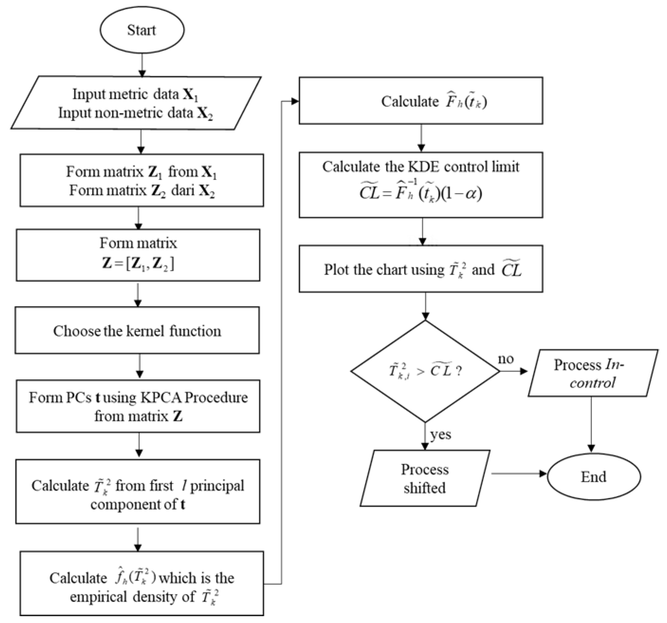
2.2. Kernel PCA Mix Control Chart Procedures

After explaining the KPCA algorithm in the previous subsection, the KPCA mix chart procedure is presented in this subsection. The main idea of KPCA mix chart is constructing the matrix Z representing the metric and nonmetric variables. There are two steps in this KPCA mix chart procedures. First, the T² statistics are calculated from matrix Z. Further, the control limit of the proposed chart is calculated using the KDE approach. These procedures are illustrated by the flowchart in Figure 2. The procedures are detailed as follows:

Statistics T² Calculation

• Form matrix $Z\hspace{0.17em}=[Z_1,Z_2]$ sized $n\times (p+m)$ where:
  • $Z_{1\hspace{0.17em}}$ sized $n\times p$ is centered on a matrix $X_1$ which is contained the metric data.
  • $Z_2$ sized $n\times m$ is centered on a matrix $G$ which is contained binary coding from every level of nonmetric data $X_2$. For example, $X_2$ has three categories such as “no defect”, “minor defect”, and “major defect” represented as 1, 2, and 3, respectively

    $$X_2=\left[\begin{array}{c}1\\ 2\\ \begin{array}{c}1\\ ⋮\end{array}\\ 3\end{array}\right],\mathrm{then} \mathrm{matrix} \mathbf{G} \mathrm{can} \mathrm{be} \mathrm{written} \mathrm{as} G=\left[\begin{array}{c}\begin{array}{ccc}1& 0& 0\end{array}\\ \begin{array}{ccc}0& 1& 0\end{array}\\ \begin{array}{c}\begin{array}{ccc}1& 0& 0\end{array}\\ \begin{array}{ccc}⋮& ⋮& ⋮\end{array}\end{array}\\ \begin{array}{ccc}0& 0& 1\end{array}\end{array}\right],$$

    where the dummy variable for “no defect” symbolized as 1 is 1 0 0, the dummy variable for “minor defect” symbolized as 2 is 0 1 0, and the dummy variable for “major defect” represented as 3 is 0 0 1.
• Calculate

  $$\tilde{Z}=N^{\frac{1}{2}}Z{M}^{\frac{1}{2}},$$

  (17)
• Choose the kernel function.
• Calculate the matrix kernel $K=K({\tilde{z}}_i,{\tilde{z}}_j)=\langle \mathsf{\Phi }({\tilde{z}}_i),\mathsf{\Phi }({\tilde{z}}_j)\rangle .$
• Calculate principal component score t as follows:

  $$t_v={\displaystyle \sum _{i=1}^n{\tilde{\alpha }}_{i,v}^{}\langle \mathsf{\Phi }(z_i),\mathsf{\Phi }(z)\rangle }={\displaystyle \sum _{i=1}^n{\tilde{\alpha }}_{i,v}^{}\tilde{K}(z_i,z)}.$$

  (18)
• From the first l principal component t, calculate the T² statistics using the following equation:

  $${\tilde{T}}_k^2={\displaystyle \sum _{v=1}^l{t}_v^{}{\lambda }_v^{-1}{t}_v^T},$$

  (19)

  where $v=1,2,\dots ,l$, and ${\lambda }_v$ eigenvalues that correspond to v-th PCs.

KDE control limit calculation

1. Estimate the empirical density of ${\tilde{T}}_k^2$ statistics using the following equation:

$${\widehat{f}}_h({\tilde{T}}_k^2)=\frac{1}{n\widehat{h}}{\displaystyle \sum _{i=1}^{n}k\left(\frac{T_{}^2-{\tilde{T}}_{k,i}^2}{\widehat{h}}\right)}$$

(20)

2. Calculate the cumulative distribution ${\widehat{F}}_h({\tilde{t}}_k)={\displaystyle \underset{0}{\overset{{\tilde{t}}_k}{\int }}{\widehat{f}}_h({\tilde{T}}_k^2)d}{\tilde{T}}_k^2$ using the trapezoid rule as follows:

$${\displaystyle \underset{{\pi }_{\min }}{\overset{{\pi }_{\max }}{\int }}{\widehat{f}}_h({\tilde{T}}_k^2)d}{\tilde{T}}_k^2\approx \frac{{\pi }_{\max }-{\pi }_{\min }}{2n}{\displaystyle \sum _{i=1}^n\left({\widehat{f}}_h\left({\tilde{T}}_{k,i}^2\right)+{\widehat{f}}_h\left({\tilde{T}}_{k,\left(i+1\right)}^2\right)\right)}$$

(21)

where ${\pi }_{\min }$ and ${\pi }_{\max }$ are the maximum and minimum value of ${\tilde{T}}_k^2$.

3. Calculate the KDE control limit using the following expression:

$$\widetilde{CL}={\widehat{F}}_h^{-1}({\tilde{t}}_k)(1-\alpha ).$$

(22)

In this paper, R statistical software was used to create the proposed KPCA mix chart and conduct the simulation studies. The Kernel-Based Machine Learning Lab (kernlab) package was used to perform the KPCA algorithm.

3. KDE Control Limit

In this section, KDE control limit of the ${\tilde{T}}_k^2$ statistics is presented for various kernel functions. Three types of kernel functions are used in this paper, such as:

• Linear Kernel K(x_i,x_j) = 〈x_i,x_j〉.
• Polynomial Kernel K(x,y) = (〈x,y〉 + 1)^d.
• Radial Basis Function (RBF) Kernel $K(x_i,x_j)=\exp \left(-{\sigma }^{*}\left|\right|x_i-x_j|{|}^2\right).$

The continuous or metric quality characteristic $X_1$ is generated from the multivariate normal distribution. In this research, the number of metric quality characteristics p is 5. Meanwhile, the nonmetric or categorical quality characteristics are generated from a multinomial distribution $X_2\sim M(n,{\theta }_1,{\theta }_2,{\theta }_3)$ with three types of parameters as follows:

• ${\theta }_1,{\theta }_2=0.3 \mathrm{and} {\theta }_3=0.4$ (balanced case),
• ${\theta }_1,{\theta }_2=0.1 \mathrm{and} {\theta }_3=0.8$ (imbalanced case),
• ${\theta }_1,{\theta }_2=0.05 \mathrm{and} {\theta }_3=0.9$ (extreme imbalanced case).

3.1. Linear Kernel

Table 1. KDE control limit of linear kernel.

	$\begin{array}{l}{\theta }_1,{\theta }_2=0.3 \\ \mathrm{and} {\theta }_3=0.4\end{array}$	$\begin{array}{l}{\theta }_1,{\theta }_2=0.1 \\ \mathrm{and} {\theta }_3=0.8\end{array}$	$\begin{array}{l}{\theta }_1,{\theta }_2=0.05 \\ \mathrm{and} {\theta }_3=0.9\end{array}$
p = 5, l = 2	10,170.30	11,267.65	11,217.93
	375.01	387.40	365.19
p = 5, l = 3	13,292.86	13,567.33	13,582.07
	376.94	385.82	379.60
p = 5, l = 4	16,007.85	15,845.09	15,942.24
	361.19	356.42	376.72

ARL₀ target is 370.

reports the KDE control limit for linear kernel when the number of continuous characteristics p is 5 and the number of PCs l = 2, 3, and 5. From the table, it can be seen that the KDE control limit produces stable ARL₀ at 370 for $\alpha =0.00273$. Additionally, it can be seen that the larger number of PCs l used the larger KDE control limit produced.

3.2. Polynomial Kernel

KDE control limits of polynomial kernel for various cases are reported in

Table 2. KDE control limit of polynomial kernel with various d for ${\theta }_1,{\theta }_2=0.3 \mathrm{and} {\theta }_3=0.4$ .

	d
	1	2	3
p = 5, l = 2	10,115.98	32,409.33	71,318.15
	355.84	804.52	844.36
p = 5, l = 3	13,129.43	39,586.61	83,200.83
	358.20	774.80	815.38
p = 5, l = 4	15,708.87	48,741.28	90,609.87
	386.68	812.37	696.31

ARL₀ target is 370.

,

Table 3. KDE control limit of polynomial kernel with various d for ${\theta }_1,{\theta }_2=0.1 \mathrm{and} {\theta }_3=0.8$ .

	d
	1	2	3
p = 5, l = 2	10,665.10	19,383.63	57,755.22
	371.39	487.68	755.76
p = 5, l = 3	13,316.01	24,878.64	71,965.38
	385.64	717.66	699.74
p = 5, l = 4	15,864.00	29,099.03	81,079.33
	351.55	656.43	620.34

ARL₀ target is 370.

and

Table 4. KDE control limit of polynomial kernel with various d for ${\theta }_1,{\theta }_2=0.05 \mathrm{and} {\theta }_3=0.9$ .

	d
	1	2	3
p = 5, l = 2	11,293.83	16,354.36	48,299.77
	379.08	542.78	668.36
p = 5, l = 3	13,476.47	22,357.91	119,229.20
	354.44	787.47	957.12
p = 5, l = 4	15,820.29	26,376.10	77,170.29
	351.76	830.91	631.40

ARL₀ target is 370.

. According to the results, the larger the d used, the larger the ARL₀ produced. In this case, the ARL₀ that is close to the theoretical is achieved when the parameter of the polynomial kernel is 1 (d = 1). Moreover, similar to the linear kernel, KDE control limit is larger for the larger number of principal components used.

3.3. RBF Kernel

Table 5. KDE control limit of RBF kernel with various ${\sigma }^{*}$ for ${\theta }_1,{\theta }_2=0.3 \mathrm{and} {\theta }_3=0.4$.

	${\mathit{\sigma }}^{*}$
	0.001	0.005	0.01	0.05	0.1
p = 5, l = 2	10,490.03	9974.92	9358.18	6338.11	5570.16
	388.28	381.70	418.82	404.65	512.10
p = 5, l = 3	12,854.18	12,165.33	11,727.51	7129.09	6302.07
	367.22	394.55	390.09	900.73	1000.00
p = 5, l = 4	16,197.98	14,669.40	13,256.48	7799.56	6556.82
	361.66	355.83	418.54	1000.00	904.12

ARL₀ target is 370.

,

Table 6. KDE control limit of RBF kernel with various ${\sigma }^{*}$ for ${\theta }_1,{\theta }_2=0.1 \mathrm{and} {\theta }_3=0.8$.

	${\mathit{\sigma }}^{*}$
	0.001	0.005	0.01	0.05	0.1
p = 5, l = 2	10,464.28	9642.60	9939.38	6487.39	5731.99
	369.76	366.09	468.92	477.56	584.15
p = 5, l = 3	12,714.55	13,059.87	11,763.30	7276.46	6496.19
	360.03	385.56	444.63	962.98	1000.00
p = 5, l = 4	16,821.44	14,567.58	13,399.80	7999.69	6759.66
	386.13	359.66	406.92	1000.00	1000.00

ARL₀ target is 370.

and

Table 7. KDE control limit of RBF kernel with various ${\sigma }^{*}$ for ${\theta }_1,{\theta }_2=0.05 \mathrm{and} {\theta }_3=0.9$.

	${\mathit{\sigma }}^{*}$
	0.001	0.005	0.01	0.05	0.1
p = 5, l = 2	11,379.40	10,474.76	9693.14	6445.41	5714.85
	386.22	385.89	358.27	463.50	687.76
p = 5, l = 3	13,524.98	12,872.44	11,690.72	7353.56	6392.95
	361.81	443.36	436.45	1000.00	1000.00
p = 5, l = 4	15,611.95	14,734.50	14,882.03	7874.67	6690.34
	354.36	397.19	437.90	1000.00	1000.00

ARL₀ target is 370.

present the KDE control limit of the proposed chart for p = 5 and various proportions of nonmetric data. From the tables, it can be seen that the smaller the hyperparameter ${\sigma }^{*}$ used, the closer the ARL₀ to the theory (in this case is 370). In general, the ARL₀ is close to the theory when the hyperparameter ${\sigma }^{*}=0.001$. Thus, for the same case in this work, the hyperparameter ${\sigma }^{*}$ is set to 0.001.

4. Performance of the Proposed Chart

In this paper, the performance of the proposed chart to detect outlier and to detect a shift in the process is evaluated for some scenarios. Similar to the previous section, the variable quality characteristics are generated from multivariate normal distribution and the attribute quality characteristics are generated from multinomial distribution.

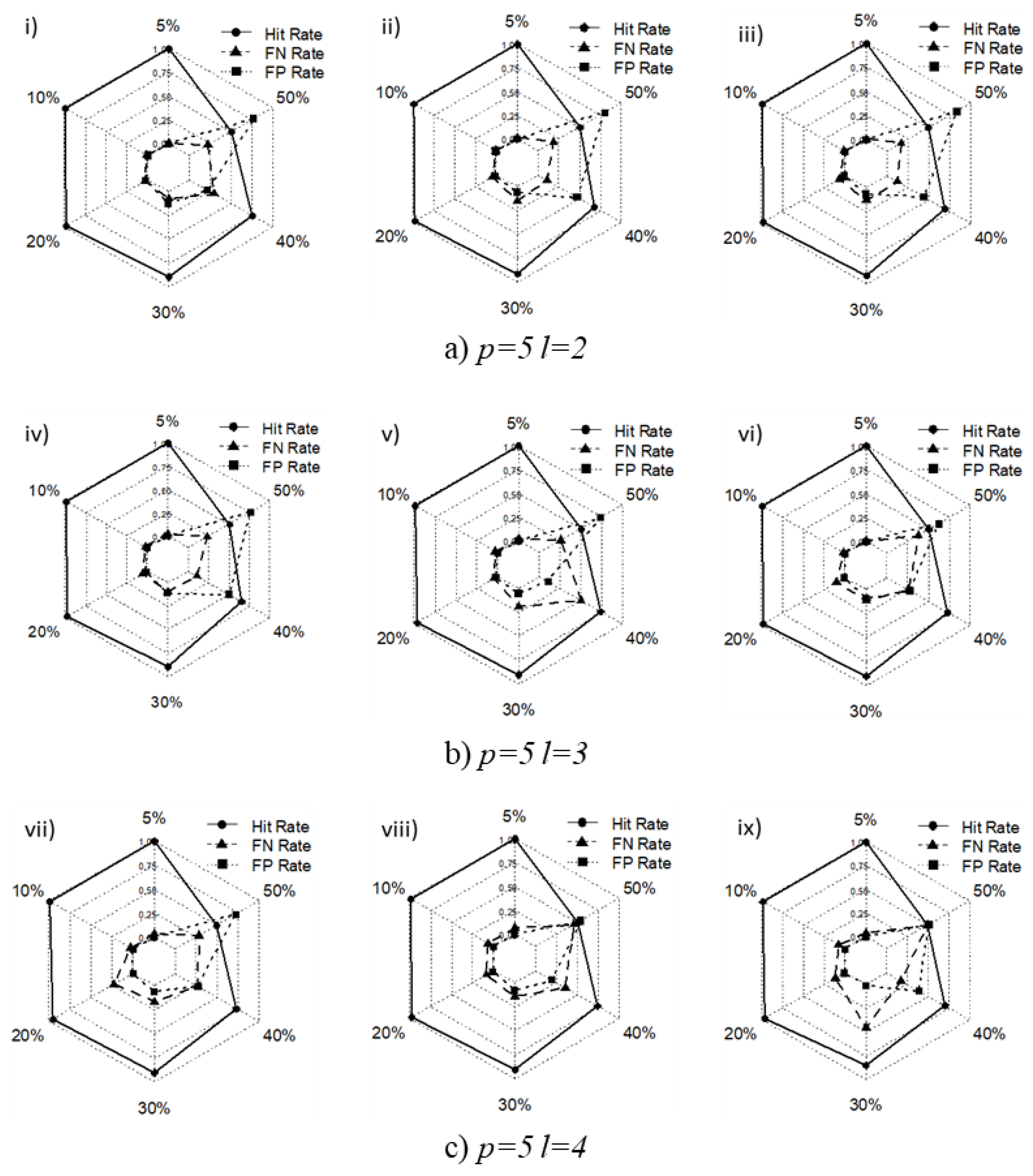
4.1. Detecting Outlier

4.1.1. Simulation Setup

In this part, the performance of the proposed chart in detecting the presence of outlier is presented. Using the same algorithm as in Ahsan et al. [20], the simulation studies was conducted 1000 times to calculate the hit rate, FN (false negative) rate, and FP (false positive) rate. The metric data $X_1$ is generated to follow the multivariate normal distribution $X_1\sim N_p(0,I).$ Meanwhile, the nonmetric data is generated to multinomial distribution $X_2\sim M(n,{\theta }_1,{\theta }_2,{\theta }_3)$. The percentage of outlier $\epsilon$ added to the clean or in-control data is set to 5%, 10%, 20%, 30%, 40%, and 50% out of the total observation. Furthermore,

Table 8. Simulation scenarios for linear, polynomial, and RBF kernel to evaluate the performance of the proposed chart in detecting outliers.

Scenario	Nonmetric Parameter	p	l
i	${\theta }_1,{\theta }_2=0.3 \mathrm{and} {\theta }_3=0.4$	5	2
ii	${\theta }_1,{\theta }_2=0.1 \mathrm{and} {\theta }_3=0.8$	5	2
iii	${\theta }_1,{\theta }_2=0.05 \mathrm{and} {\theta }_3=0.9$	5	2
iv	${\theta }_1,{\theta }_2=0.3 \mathrm{and} {\theta }_3=0.4$	5	3
v	${\theta }_1,{\theta }_2=0.1 \mathrm{and} {\theta }_3=0.8$	5	3
vi	${\theta }_1,{\theta }_2=0.05 \mathrm{and} {\theta }_3=0.9$	5	3
vii	${\theta }_1,{\theta }_2=0.3 \mathrm{and} {\theta }_3=0.4$	5	4
viii	${\theta }_1,{\theta }_2=0.1 \mathrm{and} {\theta }_3=0.8$	5	4
ix	${\theta }_1,{\theta }_2=0.05 \mathrm{and} {\theta }_3=0.9$	5	4

shows the scenarios used to assess the proposed chart performance.

4.1.2. Simulation Results

Figure 3 reports the performance evaluation results of the proposed chart with kernel linear to detect the outlier (see Appendix A

Table A1. Simulation results for linear kernel.

Scenario	$\epsilon =5\%$			$\epsilon =10\%$
	Hit Rate	FN Rate	FP Rate	Hit Rate	FN Rate	FP Rate
i	0.9990	0.0082	0.0006	0.9968	0.0126	0.0022
ii	0.9989	0.0108	0.0005	0.9949	0.0072	0.0048
iii	0.9980	0.0034	0.0019	0.9972	0.0120	0.0018
iv	0.9985	0.0232	0.0004	0.9961	0.0197	0.0021
v	0.9985	0.0204	0.0005	0.9960	0.0295	0.0012
vi	0.9983	0.0078	0.0013	0.9961	0.0208	0.0020
vii	0.9981	0.0340	0.0002	0.9953	0.0286	0.0021
viii	0.9963	0.0722	0.0001	0.9932	0.0627	0.0006
ix	0.9978	0.0402	0.0002	0.9913	0.0834	0.0004
Scenario	$\epsilon =20\%$			$\epsilon =30\%$
	Hit Rate	FN Rate	FP Rate	Hit Rate	FN Rate	FP Rate
i	0.9762	0.0316	0.0219	0.8892	0.0734	0.1269
ii	0.9784	0.0414	0.0166	0.9127	0.1515	0.0597
iii	0.9802	0.0679	0.0078	0.9105	0.1313	0.0716
iv	0.9761	0.0537	0.0164	0.8920	0.0974	0.1125
v	0.9733	0.0420	0.0229	0.9080	0.1916	0.0494
vi	0.9738	0.1040	0.0068	0.8993	0.1173	0.0936
vii	0.9521	0.2320	0.0019	0.9021	0.1719	0.0661
viii	0.9737	0.0873	0.0110	0.8993	0.1448	0.0818
ix	0.9705	0.1144	0.0083	0.8563	0.4560	0.0099
Scenario	$\epsilon =40\%$			$\epsilon =50\%$
	Hit Rate	FN Rate	FP Rate	Hit Rate	FN Rate	FP Rate
i	0.7491	0.2988	0.2190	0.5001	0.2254	0.7745
ii	0.6728	0.1134	0.4698	0.5013	0.1903	0.8070
iii	0.6852	0.1269	0.4401	0.4985	0.1686	0.8345
iv	0.6569	0.1056	0.5015	0.5002	0.2320	0.7677
v	0.7377	0.5011	0.1032	0.5009	0.2608	0.7374
vi	0.7320	0.2549	0.2768	0.5012	0.3773	0.6203
vii	0.7293	0.2701	0.2712	0.4969	0.2847	0.7215
viii	0.7405	0.3587	0.1935	0.5000	0.4616	0.5385
ix	0.6984	0.1764	0.3851	0.4993	0.4956	0.5057

for the detailed results). According to the results, the increase in the proportion of outliers added to the clean data causes a decrease in performance which can be seen from a decrease in the hit rate value. Moreover, for this case, the usage of kernel linear in kernel PCA mix chart is still reasonable for 30% outlier added to the clean data which can be seen from the high hit rate value produced (around 0.85–0.9). The performance of the proposed chart with the polynomial kernel in detecting outliers is presented in Figure 4 (see Appendix A

Table A2. Simulation results for polynomial kernel.

Scenario	$\epsilon =5\%$			$\epsilon =10\%$
	Hit Rate	FN Rate	FP Rate	Hit Rate	FN Rate	FP Rate
i	0.9989	0.0168	0.0003	0.9970	0.0156	0.0016
ii	0.9991	0.0118	0.0004	0.9969	0.0131	0.0019
iii	0.9990	0.0094	0.0006	0.9964	0.0323	0.0005
iv	0.9985	0.0140	0.0008	0.9948	0.0471	0.0006
v	0.9987	0.0124	0.0008	0.9958	0.0329	0.0011
vi	0.9984	0.0184	0.0008	0.9953	0.0118	0.0039
vii	0.9964	0.0714	0.0001	0.9948	0.0374	0.0016
viii	0.9981	0.0250	0.0007	0.9933	0.0621	0.0005
ix	0.9968	0.0614	0.0001	0.9948	0.0388	0.0015
Scenario	$\epsilon =20\%$			$\epsilon =30\%$
	Hit Rate	FN Rate	FP Rate	Hit Rate	FN Rate	FP Rate
i	0.9775	0.0338	0.0197	0.9109	0.1282	0.0724
ii	0.9805	0.0531	0.0110	0.9012	0.1002	0.0982
iii	0.9791	0.0405	0.0160	0.8878	0.0735	0.1287
iv	0.9728	0.1147	0.0053	0.9061	0.1607	0.0652
v	0.9751	0.0462	0.0195	0.9006	0.1217	0.0898
vi	0.9758	0.0459	0.0188	0.9002	0.2621	0.0302
vii	0.9718	0.0489	0.0230	0.8961	0.1312	0.0922
viii	0.9721	0.0539	0.0214	0.8999	0.2430	0.0389
ix	0.9719	0.1062	0.0086	0.8850	0.1042	0.1196
Scenario	$\epsilon =40\%$			$\epsilon =50\%$
	Hit Rate	FN Rate	FP Rate	Hit Rate	FN Rate	FP Rate
i	0.7061	0.1532	0.3877	0.5009	0.2100	0.7882
Ii	0.7352	0.2314	0.2870	0.4996	0.2009	0.8000
Iii	0.7137	0.1764	0.3595	0.5001	0.2589	0.7410
Iv	0.6933	0.1531	0.4091	0.4985	0.3272	0.6759
V	0.7368	0.2681	0.2598	0.4986	0.2994	0.7034
vi	0.7231	0.2207	0.3143	0.4988	0.3352	0.6671
vii	0.7159	0.2166	0.3291	0.4999	0.2743	0.7258
viii	0.7226	0.2461	0.2982	0.4999	0.2245	0.7757
ix	0.7330	0.2971	0.2469	0.4997	0.3320	0.6686

for detailed results). In this case, the parameter of the polynomial kernel is 1 (based on the result from the previous section). Similar to the previous results, the larger the outlier added to the clean data the smaller the hit rate value. According to its hit rate, the polynomial kernel is still in a good performance for 30% outlier added to the in-control data. Similar results also occur in RBF Kernel (see Figure 5 and Appendix A

Table A3. Simulation results for RBF kernel.

Scenario	$\epsilon =5\%$			$\epsilon =10\%$
	Hit Rate	FN Rate	FP Rate	Hit Rate	FN Rate	FP Rate
i	0.9991	0.0094	0.0005	0.9976	0.0152	0.0010
ii	0.9993	0.0086	0.0003	0.9977	0.0153	0.0009
iii	0.9989	0.0060	0.0008	0.9972	0.0211	0.0008
iv	0.9987	0.0123	0.0007	0.9959	0.0301	0.0012
v	0.9986	0.0109	0.0009	0.9956	0.0340	0.0011
vi	0.9987	0.0198	0.0004	0.9959	0.0275	0.0015
vii	0.9979	0.0124	0.0016	0.9952	0.0308	0.0019
viii	0.9975	0.0462	0.0001	0.9955	0.0317	0.0014
ix	0.9984	0.0184	0.0007	0.9949	0.0426	0.0009
Scenario	ε = 20%			ε = 30%
	Hit Rate	FN Rate	FP Rate	Hit Rate	FN Rate	FP Rate
i	0.9801	0.0337	0.0165	0.8822	0.0590	0.1429
ii	0.9778	0.0291	0.0204	0.9154	0.1205	0.0692
iii	0.9824	0.0508	0.0093	0.9099	0.2463	0.0231
iv	0.9728	0.0387	0.0244	0.9007	0.1158	0.0923
v	0.9660	0.0265	0.0359	0.9045	0.1338	0.0791
vi	0.9745	0.0440	0.0209	0.8812	0.0776	0.1365
vii	0.9648	0.1655	0.0026	0.9017	0.1300	0.0848
viii	0.9750	0.0538	0.0177	0.9082	0.1758	0.0558
ix	0.9700	0.1341	0.0040	0.9072	0.1675	0.0608
Scenario	ε = 40%			ε = 50%
	Hit Rate	FN Rate	FP Rate	Hit Rate	FN Rate	FP Rate
i	0.7361	0.2238	0.2906	0.4996	0.2591	0.7416
ii	0.7349	0.2098	0.3019	0.5006	0.4056	0.5933
iii	0.7350	0.2118	0.3004	0.4982	0.2819	0.7217
iv	0.7202	0.2077	0.3279	0.5014	0.2229	0.7744
v	0.7070	0.1784	0.3694	0.5005	0.6262	0.3728
vi	0.7000	0.1662	0.3892	0.5019	0.2490	0.7472
vii	0.7189	0.2161	0.3244	0.5001	0.3647	0.6351
viii	0.7359	0.2788	0.2544	0.4991	0.3117	0.6902
ix	0.7325	0.2540	0.2764	0.5004	0.2676	0.7316

). Using the hyperparameter ${\sigma }^{*}=0.001,$ the performance of the proposed chart is still good for smaller than 40% outlier added. When more than 40% outlier added to the in-control data, the misdetection for this case occurs due to the large false alarm produced. This happens because the proposed chart declares the actual in-control observations as the outliers. Thus, to improve the performance of the proposed chart in detecting outliers, the new method needs to overcome this issue.

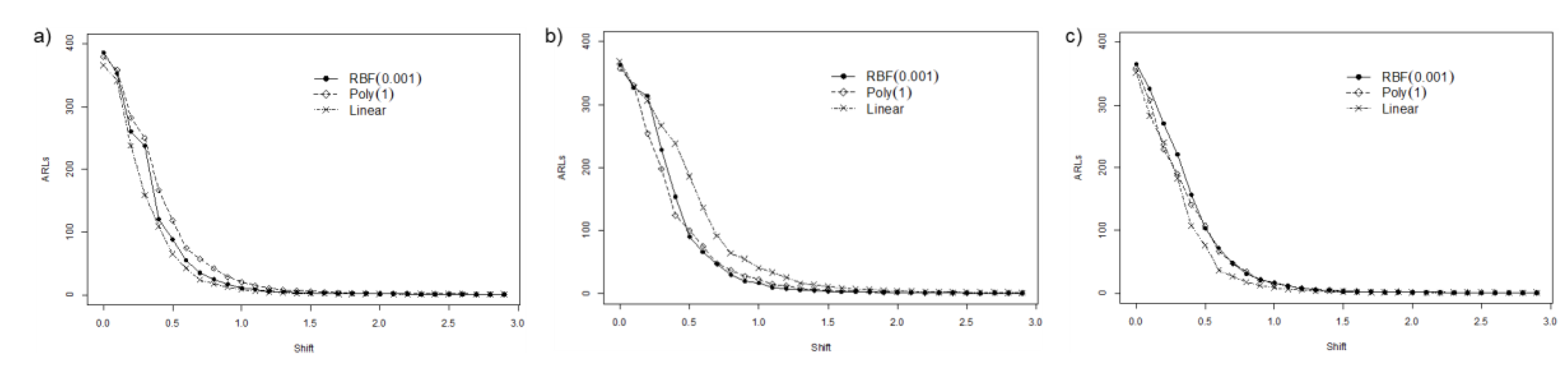
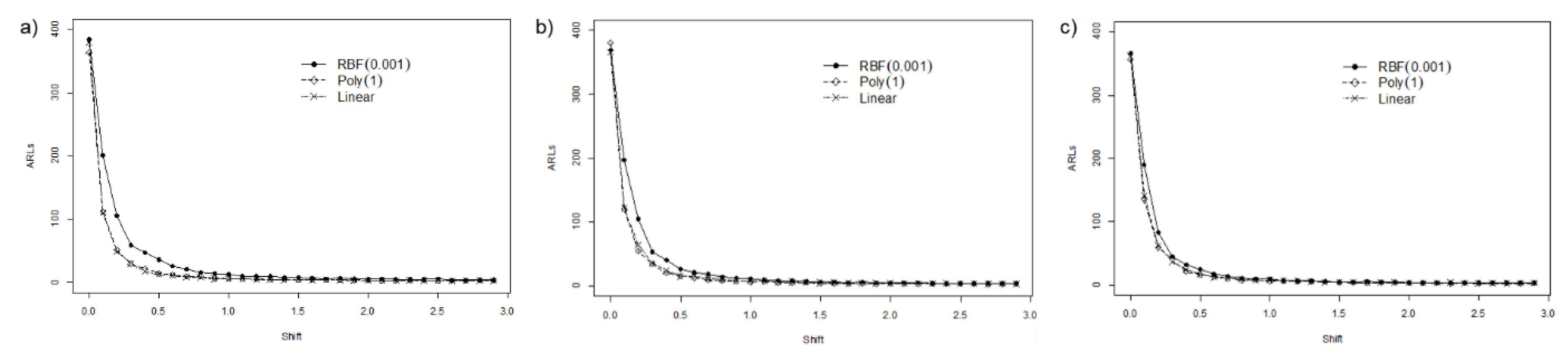
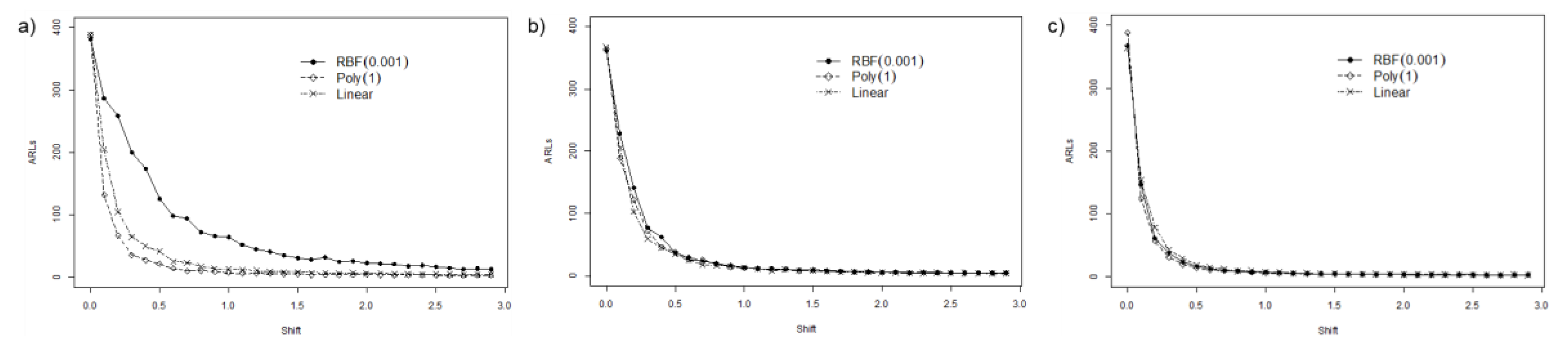
4.2. Detecting Shift in the Process

The performance of the proposed chart is evaluated to detect a shift in the process using the average run length (ARL) criterion. This chart is also evaluated using several scenarios based on the proportion of the nonmetric parameter and kernel function. Moreover, the control limits used in this simulation are taken from the previous section.

4.2.1. Extreme Imbalanced

In this subsection, the performance of the proposed chart is evaluated when the variable characteristics are generated from the multivariate normal distribution $N_p(0,I)$ and the attribute characteristics are generated from a multinomial distribution with extreme imbalanced parameter (${\theta }_1,{\theta }_2=0.05 \mathrm{and} {\theta }_3=0.9$). For p = 5 and l = 2, the evaluation results for various kernel function are visualized in Figure 6a. From the results, it can be seen that ARL₀ for all cases is around 370. Additionally, it can be concluded that the proposed chart can detect the shift in the process, which can be seen from the smaller ARL₁ value for the larger shift given. According to the figure, the ARLs value for the kernel RBF and linear are not significantly different. Furthermore, the kernel function for this case did not performed well compared to the two kernel functions.

Figure 6b depicts the performance evaluation results from the kernel PCA mix control chart for p = 5 and l = 3 with various kernel functions and extreme imbalanced proportion of categorical quality characteristics. It can be seen from the table that the proposed chart can detect a shift in the process which can be seen from smaller ARL₁ for the larger shift. For the smaller shift, the polynomial kernel produces a better performance compared to the RBF kernel which can be seen from the smaller ARL₁ owned. On the other hand, for the larger shift, the RBF kernel outperforms the polynomial kernel. For this case, the linear kernel does not perform well compared to the other kernel functions.

Figure 6c presents the ARLs of the proposed chart for ${\theta }_1,{\theta }_2=0.05 \mathrm{and} {\theta }_3=0.9$ and p = 5 and l = 4. From the figure it can be seen the difference between the kernel functions used. In general, for all kernel functions used, it can be said that the proposed chart can detect the shift in the process which can be seen from the smaller ARL₁ value for the larger shift. In this case, the similar performance from all kernel functions compared can be seen. However, for the small shift, the linear kernel produces a slightly better performance compared to the other kernels. The detailed results for this case can be found in Appendix A

Table A4. ARLs for θ₁, θ₂ = 0.05, θ₃ = 0.9, p = 5, and l = 2.

Shift		Kernel
δμ	δθ	RBF (0.001)	Poly (1)	Linear
0	0	386.221	379.075	365.194
0.1	0.0025	353.105	358.055	341.855
0.2	0.0050	260.201	282.095	237.335
0.3	0.0075	236.995	249.421	159.401
0.4	0.0100	119.915	166.745	109.505
0.5	0.0125	88.045	117.945	65.1308
0.6	0.0150	54.982	74.185	42.411
0.7	0.0175	35.195	57.105	24.155
0.8	0.0200	25.005	42.295	17.541
0.9	0.0225	16.545	28.530	12.075
1.0	0.0250	10.751	20.582	9.195
1.1	0.0275	8.307	14.291	6.815
1.2	0.0300	5.895	10.425	4.335
1.3	0.0325	4.615	8.222	3.441
1.4	0.0350	4.164	6.685	2.593
1.5	0.0375	2.811	5.565	2.445

,

Table A5. ARLs for θ₁, θ₂ = 0.05 and θ₃ = 0.9, p = 5, and l = 3.

Shift		Kernel
δμ	δθ	RBF (0.001)	Poly (1)	Linear
0	0	362.455	357.21	368.175
0.1	0.0025	326.510	330.370	328.430
0.2	0.0050	314.055	253.810	305.860
0.3	0.0075	227.840	197.685	266.260
0.4	0.0100	153.770	124.415	238.035
0.5	0.0125	90.460	99.950	185.685
0.6	0.0150	66.235	75.310	136.395
0.7	0.0175	47.225	47.925	91.755
0.8	0.0200	30.040	36.930	64.465
0.9	0.0225	20.005	27.735	55.045
1.0	0.0250	16.620	22.370	40.715
1.1	0.0275	9.930	15.050	34.060
1.2	0.0300	7.560	12.555	25.985
1.3	0.0325	5.780	7.225	16.330
1.4	0.0350	4.480	6.640	14.010
1.5	0.0375	3.925	5.225	10.945

and

Table A6. ARLs for θ₁, θ₂ = 0.05 and θ₃ = 0.9, p = 5, and l = 4.

Shift		Kernel
δμ	δθ	RBF (0.001)	Poly (1)	Linear
0	0	364.425	359.040	351.510
0.1	0.0025	325.890	307.205	282.950
0.2	0.0050	270.730	229.495	240.455
0.3	0.0075	220.725	190.665	182.670
0.4	0.0100	157.060	141.245	107.775
0.5	0.0125	103.130	107.685	76.505
0.6	0.0150	71.660	66.605	37.040
0.7	0.0175	47.840	47.645	26.845
0.8	0.0200	31.330	34.700	17.955
0.9	0.0225	21.765	20.820	12.165
1.0	0.0250	16.580	15.775	8.985
1.1	0.0275	11.385	11.305	6.610
1.2	0.0300	8.025	7.890	5.160
1.3	0.0325	5.815	5.665	3.545
1.4	0.0350	4.875	4.840	2.995
1.5	0.0375	3.655	3.115	2.515

.

4.2.2. Imbalanced

In this part, the performance of the proposed chart for the imbalanced parameter of the nonmetric characteristics with various kernel functions are presented. Figure 7a shows the ARLs of the proposed chart for ${\theta }_1,{\theta }_2=0.1,\hspace{0.17em}\hspace{0.17em}{\theta }_3=0.8$, p = 5, and l = 2 with various kernel functions used. According to the table, it can be said that the proposed chart is able to detect a shift in the process indicated by the smaller the value of ARL₁ when the process shift gets larger. For this case, the best performance is produced by the linear and polynomial kernels. On the other hand, the RBF kernel does not perform well for this scenario.

The performance of the proposed chart in detecting the shift in process for ${\theta }_1,{\theta }_2=0.1,\hspace{0.17em}\hspace{0.17em}{\theta }_3=0.8$, p = 5, and l = 3 is presented in Figure 7b. In general, the proposed chart can detect the shift for all kernel functions used. According to the figure, it can be seen that the linear and polynomial kernels have similar performance. For this case, these two kernel functions outperform the performance of RBF kernel. Furthermore, Figure 7c reports the performance of the proposed chart with various kernel functions for ${\theta }_1,{\theta }_2=0.1,\hspace{0.17em}\hspace{0.17em}{\theta }_3=0.8$, p = 5, and l = 3. According to the figure, the best performance for this case is performed by the linear and polynomial kernel. The detailed results for this case can be found in Appendix A

Table A7. ARLs for θ₁, θ₂ = 0.1 and θ₃ = 0.8, p = 5, and l = 2.

Shift		Kernel
δμ	δθ	RBF (0.001)	Poly (1)	Linear
0	0	384.025	362.975	378.955
0.1	0.0025	201.185	112.091	110.12
0.2	0.0050	105.521	51.482	48.485
0.3	0.0075	58.972	28.981	29.690
0.4	0.0100	46.851	21.675	17.275
0.5	0.0125	36.065	14.685	13.241
0.6	0.0150	25.685	12.135	11.015
0.7	0.0175	20.352	9.515	8.195
0.8	0.0200	16.151	8.755	7.760
0.9	0.0225	14.222	6.542	5.775
1.0	0.0250	12.701	6.163	5.631
1.1	0.0275	10.141	5.621	5.352
1.2	0.0300	10.111	5.210	4.605
1.3	0.0325	9.370	5.005	4.825
1.4	0.0350	8.001	4.655	3.362
1.5	0.0375	8.025	3.855	4.265

,

Table A8. ARLs for θ₁, θ₂ = 0.1 and θ₃ = 0.8, p = 5, and l = 3.

Shift		Kernel
δμ	δθ	RBF (0.001)	Poly (1)	Linear
0	0	369.025	380.04	365.145
0.1	0.0025	196.880	120.265	121.500
0.2	0.0050	104.580	54.185	64.130
0.3	0.0075	52.845	33.930	34.475
0.4	0.0100	40.210	20.265	23.995
0.5	0.0125	25.925	15.600	14.590
0.6	0.0150	20.940	12.755	14.920
0.7	0.0175	17.880	8.760	11.355
0.8	0.0200	13.400	8.225	9.655
0.9	0.0225	12.105	7.480	7.850
1.0	0.0250	10.355	5.605	7.360
1.1	0.0275	8.620	6.270	6.935
1.2	0.0300	7.725	5.050	5.860
1.3	0.0325	7.920	5.080	5.810
1.4	0.0350	6.870	4.870	4.960
1.5	0.0375	6.020	4.180	4.745

and

Table A9. ARLs for θ₁, θ₂ = 0.1 and θ₃ = 0.8, p = 5, and l = 4.

Shift		Kernel
δμ	δθ	RBF (0.001)	Poly (1)	Linear
0	0	366.170	356.350	360.710
0.1	0.0025	189.895	135.420	141.050
0.2	0.0050	82.905	58.890	62.395
0.3	0.0075	44.645	40.855	36.430
0.4	0.0100	31.450	21.180	24.260
0.5	0.0125	24.900	16.725	16.325
0.6	0.0150	17.610	13.455	12.685
0.7	0.0175	14.075	10.630	9.945
0.8	0.0200	10.665	7.650	9.210
0.9	0.0225	10.065	8.325	7.005
1.0	0.0250	9.725	6.200	7.590
1.1	0.0275	7.095	6.420	6.990
1.2	0.0300	7.165	5.600	6.210
1.3	0.0325	6.390	5.310	5.510
1.4	0.0350	6.035	4.740	4.360
1.5	0.0375	5.060	4.515	4.570

.

4.2.3. Balanced

In this subsection, the performance of the proposed chart to detect a shift in the process for the balanced proportion of the nonmetric data is presented. Some scenarios based on the kernel function and number of the PCs l used are used to assess the performance of the proposed chart. For the balanced nonmetric data with p = 5 and l = 2, the proposed chart can detect the shift in the process according to its ARL₁ values for all kernel functions (see Figure 8a). For this case, the linear and polynomial kernel outperform the performance of the RBF kernel. Moreover, the best performance for this case is presented by the polynomial kernel.

Figure 8b shows the ARLs of the proposed chart for a balanced proportion of the nonmetric parameter with p = 5 and l = 3. For this case, all kernel functions demonstrate good performance as can be seen in Figure 8b. For a small shift, the polynomial kernel shows a great performance which can be found from the smaller ARL₁ produced. On the other hand, the RBF kernel outperforms the other kernel functions for the large shift. This similar performance also happens for p = 5 and l = 3, which can be seen in Figure 8c. According to the figure, the kernel polynomial has a slightly better performance for the small shift compared to the other kernel functions. The detailed results for this case can be found in Appendix A

Table A10. ARLs for θ₁, θ₂ = 0.3 and θ₃ = 0.4, p = 5, and l = 2.

Shift		Kernel
δμ	δθ	RBF (0.001)	Poly (1)	Linear
0	0	380.765	388.43	388.155
0.1	0.0025	286.715	131.855	205.025
0.2	0.0050	258.211	66.763	104.961
0.3	0.0075	199.535	35.440	64.611
0.4	0.0100	174.015	27.561	50.075
0.5	0.0125	125.242	20.835	41.332
0.6	0.0150	98.741	13.985	25.425
0.7	0.0175	94.721	10.721	23.351
0.8	0.0200	72.552	10.385	17.281
0.9	0.0225	66.411	8.961	14.015
1.0	0.0250	64.092	6.990	13.272
1.1	0.0275	51.721	6.205	12.245
1.2	0.0300	44.495	6.695	11.131
1.3	0.0325	41.312	6.081	8.565
1.4	0.0350	35.025	5.622	8.465
1.5	0.0375	31.112	5.361	8.425

,

Table A11. ARLs for θ₁, θ₂ = 0.3 and θ₃ = 0.4, p = 5, and l = 3.

Shift		Kernel
δμ	δθ	RBF (0.001)	Poly (1)	Linear
0	0	360.92	364.295	366.095
0.1	0.0025	228.395	189.135	205.490
0.2	0.0050	141.870	121.995	102.540
0.3	0.0075	77.115	71.655	59.360
0.4	0.0100	61.580	46.030	45.345
0.5	0.0125	36.800	38.575	34.255
0.6	0.0150	29.860	26.030	25.575
0.7	0.0175	23.410	26.030	17.965
0.8	0.0200	19.785	19.700	16.910
0.9	0.0225	16.905	14.245	15.370
1.0	0.0250	13.835	12.510	13.815
1.1	0.0275	11.890	11.980	11.430
1.2	0.0300	11.705	10.165	8795
1.3	0.0325	9.845	11.230	10.145
1.4	0.0350	9.350	8.155	8.335
1.5	0.0375	9.485	9.370	8.080

and

Table A12. ARLs for θ₁, θ₂ = 0.3 and θ₃ = 0.4, p = 5, and l = 4.

Shift		Kernel
δμ	δθ	RBF (0.001)	Poly (1)	Linear
0	0	367.040	388.005	363.535
0.1	0.0025	146.845	124.230	153.925
0.2	0.0050	61.075	56.070	78.945
0.3	0.0075	37.595	30.505	43.010
0.4	0.0100	24.050	19.800	29.545
0.5	0.0125	16.650	14.650	18.340
0.6	0.0150	12.310	10.640	15.205
0.7	0.0175	9.255	10.055	12.315
0.8	0.0200	8.790	9.055	9.130
0.9	0.0225	7.825	6.900	9.840
1.0	0.0250	7.550	6.095	6.970
1.1	0.0275	6.245	5.545	7.615
1.2	0.0300	5.815	5.490	5.315
1.3	0.0325	4.900	5.025	5.975
1.4	0.0350	4.920	4.720	4.730
1.5	0.0375	4.665	4.525	5.150

.

4.3. Summary and Discussion

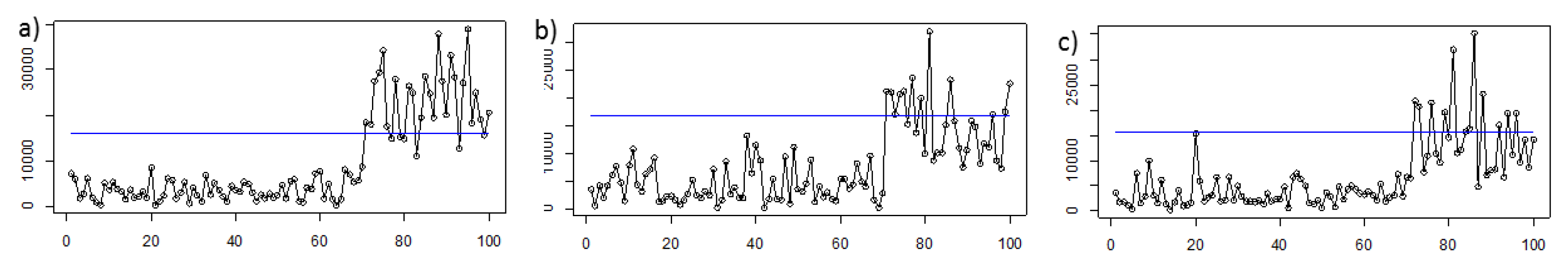
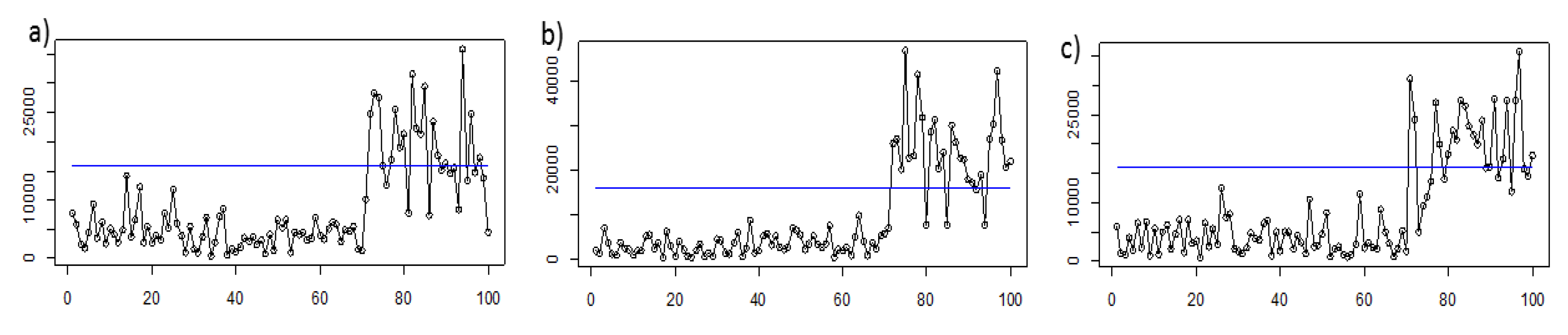
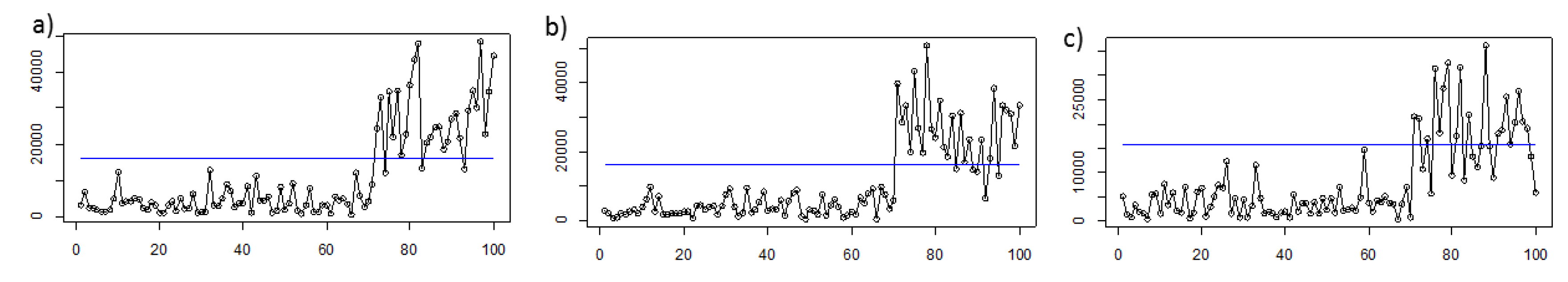
In this section, the summary of simulation studies and discussion about the performance of the proposed KPCA mix chart are presented. The simulation studies were conducted to evaluate the performance of the proposed chart in detecting outlier and process shift. In detecting outliers, it can be found that the KPCA mix chart still has better performance for 30% outlier added to the clean data. In general, for more than 30% outlier added, the misdetection is mainly caused by the high FP rate value (see Appendix A Table A1, Table A2 and Table A3).

Table 9. Summary of the proposed chart performance in detecting shift in the process for various scenarios and kernel functions.

Parameter of Nonmetric Data	l	Kernel Function
		RBF	Polynomial	Linear
Balanced	2		⁂●
	3		⁂●	⁂●
	4	⁂●	⁂●
Imbalanced	2		⁂●
	3		⁂●	⁂●
	4		⁂●	⁂●
Extreme Imbalanced	2	●		●
	3	●	●
	4			●

● represents better performance for a small shift. ⁂ represents better performance for the large shift.

summarizes the proposed KPCA mix chart performance in detecting process shift for all scenarios. The sign ● symbolizes the better performance for a small shift while the sign ⁂ represents the better performance for the large shift. Based on the results, the polynomial kernel demonstrates good performance in the balanced and imbalanced cases for both small and large shifts in the process. On the other hand, for the extreme imbalanced parameter of the nonmetric data, the RBF and linear kernels show a better performance when it is used to monitor a small shift.

Based on the summary of simulation studies discussed, some limitations are found. First, the proposed KPCA mix chart is producing more false alarm when the larger outlier is added in simulations. Second, there is no superior kernel functions for all cases. Third, executing the KPCA mix chart requires more computational time due to the complexity of the kernel function. To overcome these problems, new methods for calculating the control limit and robust estimator are needed to reduce the false alarm when more outliers are added. Additionally, discovering new kernel functions and using the Fast KPCA method can improve the accuracy and speed of the computation of the proposed chart.

5. Applications

In this section, the proposed chart is applied for the simulated and real data. First, some scenarios of data are given in order to see the ability of the proposed chart in detecting mean shift. Second, the proposed chart is applied to monitor the real data and its monitoring result is compared with the PCA mix chart [19].

5.1. Simulated Data

Table 10. Scenarios of simulated data for proposed chart application.

Scenario	${\mathit{\theta }}_1$	${\mathit{\theta }}_2$	${\mathit{\theta }}_3$	p	l	In Control Mean Process μ	Shifted Mean Process ${\mathsf{\mu }}_{\mathit{s}\mathit{h}\mathit{i}\mathit{f}\mathit{t}}$
1	0.30	0.30	0.40	5	4	0	2
2	0.10	0.10	0.80	5	4	0	2
3	0.05	0.05	0.90	5	4	0	2

shows the application of the proposed chart to monitor three scenarios of data. The linear, polynomial, and RBF kernel are employed in this application. The first 70 metric observations are generated to follow the multivariate normal distribution with $\mathsf{\mu }=0$ and $\mathsf{\Sigma }=I$. Meanwhile, the remaining 30 shifted observations are generated to follow a multivariate normal distribution with ${\mathsf{\mu }}_{shift}=2$ and $\mathsf{\Sigma }=I$. Furthermore, the nonmetric data is generated to follow the multinomial distribution with a certain parameter (${\theta }_1$, ${\theta }_2$, and ${\theta }_2$) as given in Table 10.

Figure 9, Figure 10 and Figure 11 illustrate the application of the proposed chart to monitor simulated data for RBF, polynomial, and linear kernels, respectively. From the results, it can be seen that for all kernel function used, the proposed chart can correctly detect the shift in 71st observation. However, for the imbalanced proportion of nonmetric data (see scenarios 2 and 3), the shift is not clearly seen as in the balanced case when the RBF kernel is used (see Figure 9). On the other hand, the polynomial kernel has a good performance for the imbalanced and extreme imbalanced cases as depicted in Figure 10. Furthermore, compared to the polynomial kernel, the linear kernel has better performance for the balanced and imbalanced cases as presented in Figure 11.

5.2. Real Data

In this subsection, the proposed chart is applied to monitor the machine failure data used by Ahsan et al. [19] in evaluating the mixed chart based on PCA mix. The machine failure dataset has a balanced proportion of the categorical characteristics (see the complete description in [20]). Therefore, in this application, the RBF kernel is used.

Table 11. Performance comparison between the proposed kernel PCA mix ${\tilde{T}}_k^2$ chart and PCA mix chart to monitor testing dataset in machine failure data.

Criteria	Number of Observations
	PCA Mix Chart [19]	Proposed Chart with RBF Kernel [This Study]
In-control observations	247	247
Out of control observations	3	3
Success detection of in-control observations	247	246
Success detection of out-of-control observations	2	3
Misdetection of in-control observations	0	1
Misdetection of out-of-control observations	1	0

presents the performance comparison between the proposed KPCA mix and PCA mix charts in monitoring the machine failure dataset. Based on the monitoring results, it can be concluded that the proposed chart can detect all out of control observations. However, the proposed KPCA mix chart produced more false alarms than the PCA mix chart.

6. Managerial Implication

In the industrial 4.0 era, monitoring the products with control chart plays a crucial role for the enhancement of process quality. Monitoring and enhancing the process are the main purpose of the control chart by reducing the variability in the process. The traditional control charts are used to monitor one type of quality characteristics. For instance, the numerical measurements such as length or weight are monitored using a variable type control chart. On the other hand, the categorical data such as defect, color, or softness are monitored using the attribute control chart. Thus, if a corporation wants to monitor the numerical and categorical data simultaneously, they need to use two types of the chart (variable and attribute) individually which is inefficient.

The findings in this paper are in-line with the concept of continuous quality enhancement and the adaptive monitoring process. The mixed monitoring scheme, proposed in this paper, covers not only one type of quality characteristic but also the mixed variable and attribute quality characteristic in one chart. Through simulation studies, this chart was guaranteed effective in monitoring shifts in the mixed process. By using this chart, fast corrective actions for any assignable causes can be taken by the administrator due to the sensitivity of the mixed monitoring scheme. Additionally, monitoring control limits need to be readjusted for the certain time intervals. The historical in-control observation can be used to calculated new control limits by estimating its empirical distribution (asymmetric or even unknown) using the KDE method. The adjusted control limit will help the company to adapt to the new data production behavior in the future.

7. Conclusions and Future Works

In this paper, a new control chart based on kernel PCA for monitoring mixed variable (continuous data) and attribute (categorical data) quality characteristics was proposed. The principal component scores (PCs) were transformed into T² statistics in constructing the proposed method. In calculating the accurate control limit, kernel density estimation (KDE) was employed. To evaluate the performance of the proposed chart, some scenarios with various kernel function such as linear, polynomial, and radial basis function kernels were used. For in-control condition, using the KDE control limit, the proposed chart produces ARL₀ at about 370 ($\alpha =0.00273$) for all scenarios. For the shifted process, the control chart was evaluated in monitoring the outlier in phase I and process shift in phase II. In monitoring outlier, the proposed chart was successful in detecting outliers mixed with clean data. In general, for this case, the proposed chart still has a good performance in detecting up to 30% outliers added in simulations. In monitoring the shift in the process, the proposed control chart based on kernel PCA demonstrated better performance. For this case, the different result was produced for different kernel function. The polynomial kernel showed a good performance for both small and large shifts with the balanced and imbalanced proportion of categorical data. This can be concluded from the high hit rate yielded by the polynomial kernel. On the other hand, for a small shift in the process, the linear and RBF kernels demonstrated good performance for an extreme imbalanced proportion of categorical data in term of accuracy detection. Furthermore, the proposed chart was applied to monitor the simulated and real data. The proposed chart shows great performance in monitoring the simulated data in terms of success detection of the out-of-control observations. Meanwhile, in monitoring the real data, the proposed chart outperforms the performance of the conventional PCA mix chart by producing lower false alarms. As future study, the bootstrap resampling method [28] can be employed to estimate the control limit of the proposed method. Development of mixed kernel function can also be a good alternative to exchange the conventional kernel used in this study. Finally, the use of fast kernel PCA [29] can improve the computational time.

References

1. Montgomery, D.C. Introduction to Statistical Quality Control; John Wiley & Sons: New York, NY, USA, 2009; ISBN 0470169923. [Google Scholar]
2. Ahsan, M.; Mashuri, M.; Kuswanto, H.; Prastyo, D.D. Intrusion Detection System using Multivariate Control Chart Hotelling’s T2 based on PCA. Int. J. Adv. Sci. Eng. Inf. Technol. 2018, 8, 1905–1911. [Google Scholar] [CrossRef]
3. Maleki, F.; Mehri, S.; Aghaie, A.; Shahriari, H. Robust T2 control chart using median-based estimators. Qual. Reliab. Eng. Int. 2020, 36, 2187–2201. [Google Scholar] [CrossRef]
4. Ahsan, M.; Mashuri, M.; Lee, M.H.; Kuswanto, H.; Prastyo, D.D. Robust adaptive multivariate Hotelling’s T2 control chart based on kernel density estimation for intrusion detection system. Expert Syst. Appl. 2020, 145, 113105. [Google Scholar] [CrossRef]
5. Salmasnia, A.; Kaveie, M.; Namdar, M. An integrated production and maintenance planning model under VP-T2 Hotelling chart. Comput. Ind. Eng. 2018, 118, 89–103. [Google Scholar] [CrossRef]
6. Chong, N.L.; Khoo, M.B.C.; Haq, A.; Castagliola, P. Hotelling’s T2 control charts with fixed and variable sample sizes for monitoring short production runs. Qual. Reliab. Eng. Int. 2019, 35, 14–29. [Google Scholar] [CrossRef] [Green Version]
7. Haq, A.; Khoo, M.B.C. An adaptive multivariate EWMA chart. Comput. Ind. Eng. 2019, 127, 549–557. [Google Scholar] [CrossRef]
8. Haq, A. One-sided and two one-sided MEWMA charts for monitoring process mean. J. Stat. Comput. Simul. 2020, 90, 699–718. [Google Scholar] [CrossRef]
9. Haq, A.; Munir, T.; Khoo, M.B.C. Dual multivariate CUSUM mean charts. Comput. Ind. Eng. 2019, 137, 106028. [Google Scholar] [CrossRef]
10. Khusna, H.; Mashuri, M.; Suhartono; Prastyo, D.D.; Lee, M.H.; Ahsan, M. Residual-based maximum MCUSUM control chart for joint monitoring the mean and variability of multivariate autocorrelated processes. Prod. Manuf. Res. 2019, 7, 364–394. [Google Scholar] [CrossRef] [Green Version]
11. Zaman, B.; Lee, M.H.; Riaz, M.; Abujiya, M.R. An improved process monitoring by mixed multivariate memory control charts: An application in wind turbine field. Comput. Ind. Eng. 2020, 142, 106343. [Google Scholar] [CrossRef]
12. Aldosari, M.S.; Aslam, M.; Srinivasa Rao, G.; Jun, C.-H. An attribute control chart for multivariate Poisson distribution using multiple dependent state repetitive sampling. Qual. Reliab. Eng. Int. 2019, 35, 627–643. [Google Scholar] [CrossRef]
13. Mashuri, M.; Wibawati; Purhadi; Irhamah. A Fuzzy Bivariate Poisson Control Chart. Symmetry 2020, 12, 573. [Google Scholar]
14. Lee, J.; Peng, Y.; Wang, N.; Reynolds, M.R., Jr. A GLR control chart for monitoring a multinomial process. Qual. Reliab. Eng. Int. 2017, 33, 1773–1782. [Google Scholar] [CrossRef]
15. Pu, X.; Li, Y.; Xiang, D. Mixed variables-attributes test plans for single and double acceptance sampling under exponential distribution. Math. Probl. Eng. 2011, 2011, 1–15. [Google Scholar] [CrossRef]
16. Aslam, M.; Azam, M.; Khan, N.; Jun, C.H. A mixed control chart to monitor the process. Int. J. Prod. Res. 2015, 53, 4684–4693. [Google Scholar] [CrossRef]
17. Aslam, M.; Khan, N.; Aldosari, M.S.; Jun, C.H. Mixed Control Charts Using EWMA Statistics. IEEE Access 2016, 4, 8286–8293. [Google Scholar] [CrossRef]
18. Wang, J.; Su, Q.; Fang, Y.; Zhang, P. A multivariate sign chart for monitoring dependence among mixed-type data. Comput. Ind. Eng. 2018, 126, 625–636. [Google Scholar] [CrossRef]
19. Ahsan, M.; Mashuri, M.; Kuswanto, H.; Prastyo, D.D.; Khusna, H. Multivariate Control Chart based on PCA Mix for Variable and Attribute Quality Characteristics. Prod. Manuf. Res. 2018, 6, 364–384. [Google Scholar] [CrossRef]
20. Ahsan, M.; Mashuri, M.; Kuswanto, H.; Prastyo, D.D.; Khusna, H. Outlier detection using PCA mix based T2 control chart for continuous and categorical data. Commun. Stat.-Simul. Comput. 2019, 1–28. [Google Scholar] [CrossRef]
21. Phaladiganon, P.; Kim, S.B.; Chen, V.C.P.; Jiang, W. Principal component analysis-based control charts for multivariate nonnormal distributions. Expert Syst. Appl. 2013, 40, 3044–3054. [Google Scholar] [CrossRef]
22. Schölkopf, B.; Smola, A.; Müller, K.-R. Kernel principal component analysis. Artif. Neural Netw.-ICANN 1997, 97, 583–588. [Google Scholar] [CrossRef]
23. Ma, X.; Zabaras, N. Kernel principal component analysis for stochastic input model generation. J. Comput. Phys. 2011, 230, 7311–7331. [Google Scholar] [CrossRef]
24. Lee, J.-M.; Yoo, C.; Choi, S.W.; Vanrolleghem, P.A.; Lee, I.-B. Nonlinear process monitoring using kernel principal component analysis. Chem. Eng. Sci. 2004, 59, 223–234. [Google Scholar] [CrossRef]
25. Stefatos, G.; Hamza, A. Ben Statistical process control using kernel PCA. In Proceedings of the 2007 Mediterranean Conference on Control & Automation, Athens, Greece, 27–29 June 2007; pp. 1–6. [Google Scholar]
26. Dong, D.; McAvoy, T.J. Nonlinear principal component analysis—Based on principal curves and neural networks. Comput. Chem. Eng. 1996, 20, 65–78. [Google Scholar] [CrossRef]
27. Boser, B.E.; Guyon, I.M.; Vapnik, V.N. A Training Algorithm for Optimal Margin Classifiers. In Proceedings of the 5th Annual Acm Workshop on Computational Learning Theory, Pittsburgh, PA, USA, 27–29 July 1992; pp. 144–152. [Google Scholar]
28. Khusna, H.; Mashuri, M.; Ahsan, M.; Suhartono, S.; Prastyo, D.D. Bootstrap Based Maximum Multivariate CUSUM Control Chart. Qual. Technol. Quant. Manag. 2018, 17, 52–74. [Google Scholar] [CrossRef]
29. Khediri, I.B.; Limam, M.; Weihs, C. Variable window adaptive Kernel Principal Component Analysis for nonlinear nonstationary process monitoring. Comput. Ind. Eng. 2011, 61, 437–446. [Google Scholar] [CrossRef]
Figure 1. Illustration of KPCA [23].
Symmetry 12 01838 g001
Figure 2. KPCA mix chart procedures.
Symmetry 12 01838 g002
Figure 3. Visualization of the hit rate, FN rate, and FP rate for all scenarios with the linear kernel for: (a) p = 5 l = 2, (b) p = 5 l = 3, and (c) p = 5 l = 4.
Symmetry 12 01838 g003
Figure 4. Visualization of the hit rate, FN rate, and FP rate for all scenarios with the polynomial kernel for: (a) p = 5 l=2, (b) p = 5 l = 3, and (c) p = 5 l = 4.
Symmetry 12 01838 g004
Figure 5. Visualization of the hit rate, FN rate, and FP rate for all scenarios with the RBF kernel for: (a) p = 5 l = 2, (b) p = 5 l = 3, and (c) p = 5 l = 4.
Symmetry 12 01838 g005
Figure 6. ARLs comparison from various kernel function with θ 1 , θ 2 = 0.05   and   θ 3 = 0.9 for (a) p = 5 and l = 2, (b) p = 5 and l = 3, and (c) p = 5 and l = 4.
Symmetry 12 01838 g006
Figure 7. ARLs comparison from various kernel function with θ 1 , θ 2 = 0.1   and   θ 3 = 0.8 for (a) p = 5 and l = 2, (b) p = 5 and l = 3, and (c) p = 5 and l = 4.
Symmetry 12 01838 g007
Figure 8. ARLs comparison from various kernel function with θ 1 , θ 2 = 0.3   and   θ 3 = 0.4 for (a) p = 5 and l = 2, (b) p = 5 and l = 3, and (c) p = 5 and l = 4.
Symmetry 12 01838 g008
Figure 9. Application of the proposed T ˜ k 2 chart with kernel RBF (0.001) for (a) scenario 1, (b) scenario 2, and (c) scenario 3.
Symmetry 12 01838 g009
Figure 10. Application of the proposed T ˜ k 2 chart with kernel polynomial (1) for (a) scenario 1, (b) scenario 2, and (c) scenario 3.
Symmetry 12 01838 g010
Figure 11. Application of the proposed T ˜ k 2 chart with kernel linear for (a) scenario 1, (b) scenario 2, and (c) scenario 3.
Symmetry 12 01838 g011