Influence of the Replacement of the Actual Plastic Orthotropy with Various Approximations of Normal Anisotropy on Residual Stresses and Strains in a Thin Disk Subjected to External Pressure

Abstract

Plastic anisotropy is very common to metallic materials. This property may significantly affect the performance of structures. However, the actual orthotropic yield criterion is often replaced with a criterion based on the assumption of normal anisotropy. The present paper aims to reveal the influence of this replacement on the distribution of strains and residual strains in a thin hollow disk under plane stress conditions. The boundary-value problem is intentionally formulated such that it is possible to obtain an exact semi-analytical solution without relaxing the boundary conditions. It is assumed that the disk is loaded by external pressure, followed by elastic unloading. The comparative analysis of the distributions of residual strains shows a significant deviation of the distribution resulting from the solutions based on the assumption of normal anisotropy from the distribution found using the actual orthotropic yield criterion. This finding shows that replacing the actual orthotropic yield criterion with the assumption of normal anisotropy may result in very inaccurate predictions. The type of anisotropy accepted is of practical importance because it usually results from such processes as drawing end extrusion with an axis of symmetry.

1. Introduction

Many metallic materials are plastically anisotropic. The orthotropic form of anisotropy is most common, arising from such metal forming processes as rolling, drawing and extrusion [1]. This material property affects both subsequent sheet metal forming processes and the performance of structures and machine parts made of the products of these processes [2]. For example, the residual stresses and, hence, the elastic springing are very sensitive to plastic anisotropy [3,4]. The effect of plastic anisotropy on the solution behavior for thin rotating disks has been revealed in [5,6,7]. However, for simplifying theoretical calculations, the real orthotropic yield criterion is often replaced with a transversely isotropic yield criterion (i.e., it is assumed that the material properties are independent of the direction within the transverse plane). This type of anisotropy is called normal anisotropy. The effect of the replacement above is usually not evaluated. The primary objective of the present paper is to evaluate this effect for a particular structure.

The assumption of normal anisotropy is often used for the analysis of various sheet metal forming processes. In [8,9,10,11,12], theoretical analyses for the elastic/plastic bending of sheet metal have been carried out to predict springback, bendability, strain and stress distributions, and the maximum load on the punch. In [13], a numerical and analytical study on the stretch flanging of V-shaped sheet metal has been presented. A non-linear correlation between the hole expansion ratio and tensile properties, including the coefficient of normal anisotropy, has been revealed in [14,15]. Many instability (or failure) criteria used for predicting the limit strain and formability of sheet metal are applicable only for normal anisotropy [16,17,18]. In [19,20,21], the influence of plastic anisotropy on the plastic behavior and failure of porous ductile materials has been studied using different modifications of the Gurson yield criterion. Still, in all these cases, the matrix is supposed to be transversely isotropic. The assumption of normal anisotropy is also used to study the effect of anisotropy on the hardness of billets after upsetting [22], and to estimate the no-rivet connection quality [23].

Moreover, the assumption of normal anisotropy is often used not only to analyze technological processes but also for the estimation of plastic anisotropy of different materials. For example, in [24], Al/Cu bimetallic sheets have been studied, and the copper layer thickness’s influence on the normal anisotropy has been reported. The normal anisotropy coefficients have also been used. The authors of [25] studied the influence of continuous annealing temperature on battery shell steel’s mechanical properties. In [26], the normal anisotropy of crystallographic orientations has been calculated to evaluate the effect of crystallographic texture on the stretch-flangeability during the hole expansion test of hot-rolled multiphase steel.

There are various expressions for calculating the parameters involved in transversely isotropic yield criteria [2,27,28,29,30]. These expressions depend on the number of directions along which the yield stress is available. Therefore, it is of interest to reveal the effect of different transversely isotropic yield criteria on the distribution of residual stresses and strains in structures. For this purpose, it is not necessary to solve a complicated boundary value problem. It is more important to derive an analytic or semi-analytic solution without relaxing any boundary conditions. In [31], the effect of replacing the exact yield criterion by transversely isotropic yield criteria on the distribution of residual stresses in a thin hollow disk subjected to external pressure and subsequent unloading has been investigated. In the present study, this analysis is extended to the distribution of residual strains. A comprehensive overview of the boundary value problem solved has been provided in [32]. This overview does not include solutions for anisotropic materials.

2. Statement of the Problem

In many cases, the actual orthotropic yield criterion (i.e., this criterion describes experimental data with sufficient accuracy) is replaced with the assumption of normal anisotropy [8,9,10,11,12,13,14,15,16,17,18,19,20,21,22,23]. The effect of this replacement on the final result is unknown. It may depend on the actual yield criterion and its approximations. In the present paper, the quadratic yield criterion proposed by Hill [33] is chosen as the actual yield criterion. However, any other criterion can play this role. Having Hill’s yield criterion, one can find parameters that are necessary for formulating any yield criterion based on the assumption of normal anisotropy. These different yield criteria are used for finding the distributions of residual stresses and strains under the same system of loading. The difference in these distributions is considered as the effect of the replacement of the actual yield criterion with approximate yield criteria.

It is seen from the above that the choice of the boundary value problem is not so crucial for the primary objective of this study. For the reason of transparency of the final result, it is desirable to have semi-analytic solutions without relaxing the equations and boundary conditions. The boundary value problem below satisfies this requirement.

Consider the deformation of a thin hollow disk of inner radius a₀ and outer radius b₀ by a uniform external pressure $p_0$, followed by unloading (Figure 1). The internal pressure is zero. It is natural to solve this boundary value problem in a cylindrical coordinate system $\left(r,\theta ,z\right)$ whose $z-$axis coincides with the axis of symmetry of the disk. Let ${\sigma }_r$, ${\sigma }_{\theta }$ and ${\sigma }_z$ be the normal stresses referred to this coordinate system. The state of stress is plane, ${\sigma }_z=0$. The stress boundary conditions are

$${\sigma }_r=0$$

(1)

for $r=a_0$ and

$${\sigma }_r=-p_0$$

(2)

for $r=b_0$.

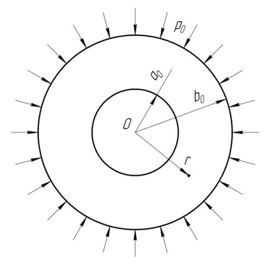
Figure 1. Schematic of the disk subjected to external pressure $p_0$.

The constitutive equations comprise Hooke’s law, the yield criterion, and its associated flow rule. It is assumed that the material of the disk is orthotropic and obeys the Hill’s quadratic yield criterion [33]. Moreover, the principal axes of anisotropy coincide with the coordinate curves of the cylindrical coordinate system. Then, since ${\sigma }_z=0$, the yield criterion is represented as

$$\left(G+H\right){\sigma }_r^2-2H{\sigma }_r{\sigma }_{\theta }+\left(H+F\right){\sigma }_{\theta }^2=1,$$

(3)

where

$$2F=\frac{1}{Y^2}+\frac{1}{Z^2}-\frac{1}{X^2},\hspace{1em}2G=\frac{1}{Z^2}+\frac{1}{X^2}-\frac{1}{Y^2},\hspace{1em}2H=\frac{1}{X^2}+\frac{1}{Y^2}-\frac{1}{Z^2}$$

(4)

and X, Y and Z are the yield stresses in tension in the radial, circumferential, and axial directions, respectively. One can also express the coefficients F, G, and H in terms of the Lankford’s coefficients $R_0$ and $R_{90}$ as [2]

$$F=\frac{1}{X^2}\frac{R_0}{R_{90}\left(R_0+1\right)},\hspace{1em}G=\frac{1}{X^2}\frac{1}{\left(R_0+1\right)},\hspace{1em}H=\frac{1}{X^2}\frac{R_0}{\left(R_0+1\right)}.$$

(5)

here, the coefficient $R_0$ corresponds to the radial direction and the coefficient $R_{90}$ to the circumferential direction. Actual orthotropic yield criteria are often approximated by the normally anisotropic yield criterion of the form

$${\sigma }_r^2-\frac{2\overline{R}}{\left(1+\overline{R}\right)}{\sigma }_r{\sigma }_{\theta }+{\sigma }_{\theta }^2={\overline{\sigma }}_s^2,$$

(6)

where ${\overline{\sigma }}_s$ is the average yield stress in tension in any direction in planes z = constant. The value of $\overline{R}$ is expressed through the Lankford’s coefficients in different directions. Several expressions are available in the literature [2,27,28,29,30]. All of them can be represented as [30]

$$\overline{R}=\{\begin{array}{ll}\frac{R_0+2{\displaystyle \sum _{i=1}^{n-2}{R}_{\Delta \alpha i}}+R_{90}}{2\left(n-1\right)}& \mathrm{if}\hspace{1em}n>2,\\ \frac{R_0+R_{90}}{2}& \mathrm{if}\hspace{1em}n=2.\end{array}$$

(7)

Similar expressions are used for the average yield stress in tension:

$${\overline{\sigma }}_s=\{\begin{array}{ll}\frac{X+2{\displaystyle \sum _{i=1}^{n-2}{\sigma }_s{}_{\Delta \alpha i}}+Y}{2\left(n-1\right)}& \mathrm{if}\hspace{1em}n>2,\\ \frac{X+Y}{2}& \mathrm{if}\hspace{1em}n=2.\end{array}$$

(8)

The difference between the expressions in [2,27,28,29,30] is in the value of n. In Equations (7) and (8), n is the number of directions in which the Lankford’s coefficients and yield stresses are measured (including the radial and circumferential directions), $R_{\Delta \alpha i}$ is the Lankford’s coefficient in the direction $\gamma =\Delta \alpha i$, ${\sigma }_s{}_{\Delta \alpha i}$ is the yield stress in tension in the direction $\gamma =\Delta \alpha i$, $\gamma$ is the angle measured from the radial direction anticlockwise, and $\Delta \alpha =\pi /\left[2\left(n-1\right)\right]$.

It is evident from Equations (1)–(3) and (6) that the solution for any yield criterion is independent of $\theta$. Moreover, the stresses ${\sigma }_r$, ${\sigma }_{\theta }$ and ${\sigma }_z$ are the principal stresses. Therefore, the only non-trivial equilibrium equation is

$$\frac{\partial {\sigma }_r}{\partial r}+\frac{{\sigma }_r-{\sigma }_{\theta }}{r}=0.$$

(9)

Let ${\epsilon }_r$, ${\epsilon }_{\theta }$ and ${\epsilon }_z$ be the normal strains referred to the cylindrical coordinate system. These strains are the principal strains. Therefore, the Hooke’s law reduces to

$$E{\epsilon }_r^e={\sigma }_r-\nu {\sigma }_{\theta },\hspace{1em}E{\epsilon }_{\theta }^e={\sigma }_{\theta }-\nu {\sigma }_r,\hspace{1em}E{\epsilon }_z^e=-\nu \left({\sigma }_r+{\sigma }_{\theta }\right).$$

(10)

here, the superscript e denotes the elastic portion of the strain components, E is the Young’s modulus, and $\nu$ is the Poisson’s ratio. The plastic flow rule associated with Yield Criterion (3) is

$${\dot{\epsilon }}_r^p=\lambda \left[\left(G+H\right){\sigma }_r-H{\sigma }_{\theta }\right],\hspace{1em}{\dot{\epsilon }}_{\theta }^p=\lambda \left[\left(F+H\right){\sigma }_{\theta }-H{\sigma }_r\right],\hspace{1em}{\dot{\epsilon }}_z^p=-\lambda \left(G{\sigma }_r+F{\sigma }_{\theta }\right)$$

(11)

and with Yield Criterion (6) is

$${\dot{\epsilon }}_r^p={\lambda }_1\left[{\sigma }_r-\frac{\overline{R}{\sigma }_{\theta }}{\left(1+\overline{R}\right)}\right],\hspace{1em}{\dot{\epsilon }}_{\theta }^p={\lambda }_1\left[{\sigma }_{\theta }-\frac{\overline{R}{\sigma }_r}{\left(1+\overline{R}\right)}\right],\hspace{1em}{\dot{\epsilon }}_z^p=-\frac{{\lambda }_1}{\left(1+\overline{R}\right)}\left({\sigma }_r+{\sigma }_{\theta }\right).$$

(12)

here, $\lambda$ and ${\lambda }_1$ are non-negative multipliers, and the superscript p denotes the plastic portion of the strain components, and the superimposed dot denotes the time derivative. The total strain components are determined as

$${\epsilon }_r={\epsilon }_r^e+{\epsilon }_r^p,\hspace{1em}{\epsilon }_{\theta }={\epsilon }_{\theta }^e+{\epsilon }_{\theta }^p,\hspace{1em}{\epsilon }_z={\epsilon }_z^e+{\epsilon }_z^p.$$

(13)

In what follows, it is convenient to use the dimensionless quantities:

$$\rho =\frac{r}{b_0},\hspace{1em}a=\frac{a_0}{b_0},\hspace{1em}k=\frac{X}{E},\hspace{1em}s=\frac{{\overline{\sigma }}_s}{X},\hspace{1em}p=\frac{p_0}{X}.$$

(14)

The present paper aims to show the effect of replacing Yield Criterion (3) with (6) on the distribution of stresses and strain at the end of loading and residual stresses and strains.

3. Stress Solution

A stress solution has been found in [31]. For the reason of readability, the main results of this solution are presented in this section.

In the case of Yield Criterion (3), the distribution of the radial and circumferential stresses in the plastic region $a_0\le r\le r_c$ (or $a\le \rho \le {\rho }_c$) is given in parametric form as

$$\begin{array}{l}\frac{{\sigma }_r}{X}=-\frac{2\sin \psi }{\sqrt{4-{\eta }^2}},\hspace{1em}\frac{{\sigma }_{\theta }}{X}=-{\eta }_1\left(\frac{\eta \sin \psi }{\sqrt{4-{\eta }^2}}+\cos \psi \right),\\ \ln \left(\frac{\rho }{a}\right)=\frac{{\eta }_1\sqrt{4-{\eta }^2}}{2\left[1+{\eta }_1\left({\eta }_1-\eta \right)\right]}\psi +\\ \hspace{1em}\hspace{1em}\hspace{1em}\hspace{1em}\hspace{1em}+\frac{\left(2-\eta {\eta }_1\right)}{2\left[1+{\eta }_1\left({\eta }_1-\eta \right)\right]}\ln \left[\frac{{\eta }_1\sqrt{4-{\eta }^2}}{{\eta }_1\sqrt{4-{\eta }^2}\cos \psi -\left(2-\eta {\eta }_1\right)\sin \psi }\right],\end{array}$$

(15)

where $\eta =2HXY$, ${\eta }_1=Y/X$, $\psi$ is an auxiliary variable, $r_c$ is the radius of the elastic/plastic boundary and ${\rho }_c$ is its dimensionless representation, ${\rho }_c=r_c/b_0$. The distribution of the radial and circumferential stresses in the elastic region $r_c\le r\le b_0$ (or ${\rho }_c\le \rho \le 1$) is given as

$$\begin{array}{l}\frac{{\sigma }_r}{X}=\frac{A\left(1-{\rho }^2\right)}{{\rho }^2}-p,\hspace{1em}\frac{{\sigma }_{\theta }}{X}=-\frac{A\left(1+{\rho }^2\right)}{{\rho }^2}-p,\\ A={\rho }_c^2\left[\frac{{\eta }_1}{2}\left(\frac{\eta \sin {\psi }_c}{\sqrt{4-{\eta }^2}}+\cos {\psi }_c\right)-\frac{\sin {\psi }_c}{\sqrt{4-{\eta }^2}}\right].\end{array}$$

(16)

Let ${\psi }_c$ be the value of $\psi$ at $\rho ={\rho }_c$. One can find ${\psi }_c$ and ${\rho }_c$ as functions of p from the following equations:

$$\begin{array}{l}\ln \left(\frac{{\rho }_c}{a}\right)=\frac{{\eta }_1\sqrt{4-{\eta }^2}}{2\left[1+{\eta }_1\left({\eta }_1-\eta \right)\right]}{\psi }_c+\\ \hspace{1em}\hspace{1em}\hspace{1em}\hspace{1em}\hspace{1em}\hspace{1em}+\frac{\left(2-\eta {\eta }_1\right)}{2\left[1+{\eta }_1\left({\eta }_1-\eta \right)\right]}\ln \left[\frac{{\eta }_1\sqrt{4-{\eta }^2}}{{\eta }_1\sqrt{4-{\eta }^2}\cos {\psi }_c-\left(2-\eta {\eta }_1\right)\sin {\psi }_c}\right],\\ \frac{\sin {\psi }_c}{\sqrt{4-{\eta }^2}}\left(1-{\rho }_c^2\right)+\frac{{\eta }_1}{2}\left(\frac{\eta \sin {\psi }_c}{\sqrt{4-{\eta }^2}}+\cos {\psi }_c\right)\left(1+{\rho }_c^2\right)=-p.\end{array}$$

(17)

Then, the radial distribution of the stresses ${\sigma }_r$ and ${\sigma }_{\theta }$ at a given value of p immediately follows from Equations (15) and (16).

In the case of Yield Criterion (6), the distribution of the radial and circumferential stresses in the plastic region $a\le \rho \le {\rho }_c$ is given in parametric form as

$$\begin{array}{l}\frac{{\sigma }_r}{{\sigma }_s}=-q_1\sin \phi ,\hspace{1em}\frac{{\sigma }_{\theta }}{{\sigma }_s}=-q_2\sin \phi -\cos \phi ,\\ \ln \left(\frac{\rho }{a}\right)=-\frac{\sqrt{1+2\overline{R}}}{2}\left\{\phi +\left(q_1-q_2\right)\ln \left[\cos \phi +\left(q_1-q_2\right)\sin \phi \right]\right\},\\ q_1=\frac{1+\overline{R}}{\sqrt{1+2\overline{R}}},\hspace{1em}{q}_2=\frac{\overline{R}}{\sqrt{1+2\overline{R}}},\end{array}$$

(18)

where $\phi$ is an auxiliary variable. The distribution of the radial and circumferential stresses in the elastic region ${\rho }_c\le \rho \le 1$ is given as

$$\begin{array}{l}\frac{{\sigma }_r}{{\sigma }_s}=\frac{A_1}{{\rho }^2}-B_1,\hspace{1em}\frac{{\sigma }_{\theta }}{{\sigma }_s}=-\frac{A_1}{{\rho }^2}-B_1,\\ B_1=\frac{1}{2}\left[\left(q_1+q_2\right)\sin {\phi }_c-\cos {\phi }_c\right],\hspace{1em}{A}_1=\frac{{\rho }_c^2}{2}\left[\left(q_1-q_2\right)\sin {\phi }_c+\cos {\phi }_c\right],\end{array}$$

(19)

where ${\phi }_c$ is the value of $\phi$ at $\rho ={\rho }_c$. It is seen from Equation (18) that

$$\ln \left(\frac{{\rho }_c}{a}\right)=-\frac{\sqrt{1+2\overline{R}}}{2}\left\{{\phi }_c+\left(q_1-q_2\right)\ln \left[\cos {\phi }_c+\left(q_1-q_2\right)\sin {\phi }_c\right]\right\}.$$

(20)

Moreover, it follows from Equations (2), (14) and (19) that

$$B_1=A_1+\frac{p}{s}.$$

(21)

Substituting Equation (19) into Equation (21) leads to

$$\left(q_1+q_2\right)\sin {\phi }_c-\cos {\phi }_c={\rho }_c^2\left[\left(q_1-q_2\right)\sin {\phi }_c+\cos {\phi }_c\right]+\frac{2p}{s}.$$

(22)

The solution of Equations (20) and (22) supplies the dependencies of ${\phi }_c$ and ${\rho }_c$ on p. Then, the radial distribution of the stresses ${\sigma }_r$ and ${\sigma }_{\theta }$ at a given value of p immediately follows from Equations (18) and (19).

The radial stress increment at the end of unloading should satisfy the boundary conditions:

$$\Delta {\sigma }_r=0$$

(23)

for $\rho =a$ and

$$\Delta {\sigma }_r=p_0$$

(24)

for $\rho =1$. Assuming that the process of unloading is purely elastic, one can find from the equilibrium equations and Hooke’s law that the solution for the radial and circumferential stress increments satisfying the boundary conditions (23) and (24) is

$$\Delta {\sigma }_r=\frac{p_0}{\left(1-a^2\right)}\left(1-\frac{a^2}{{\rho }^2}\right),\hspace{1em}\Delta {\sigma }_{\theta }=\frac{p_0}{\left(1-a^2\right)}\left(1+\frac{a^2}{{\rho }^2}\right).$$

(25)

This solution is independent of the yield criterion accepted for the stage of loading.

Let ${\sigma }_r^f$ and ${\sigma }_{\theta }^f$ be the radial and circumferential stresses at the end of loading, respectively. The residual stresses are determined from the equations ${\sigma }_r^{res}={\sigma }_r^f+\Delta {\sigma }_r$ and ${\sigma }_{\theta }^{res}={\sigma }_{\theta }^f+\Delta {\sigma }_{\theta }$. Then, using Equations (14) and (25) one can find the radial distribution of residual stresses as

$$\frac{{\sigma }_r^{res}}{X}=\frac{{\sigma }_r^f}{X}+\frac{p}{\left(1-a^2\right)}\left(1-\frac{a^2}{{\rho }^2}\right),\hspace{1em}\frac{{\sigma }_{\theta }^{res}}{X}=\frac{{\sigma }_{\theta }^f}{X}+\frac{p}{\left(1-a^2\right)}\left(1+\frac{a^2}{{\rho }^2}\right)$$

(26)

in the case of Yield Criterion (3) and

$$\frac{{\sigma }_r^{res}}{{\sigma }_s}=\frac{{\sigma }_r^f}{{\sigma }_s}+\frac{p}{s\left(1-a^2\right)}\left(1-\frac{a^2}{{\rho }^2}\right),\hspace{1em}\frac{{\sigma }_{\theta }^{res}}{{\sigma }_s}=\frac{{\sigma }_{\theta }^f}{{\sigma }_s}+\frac{p}{s\left(1-a^2\right)}\left(1+\frac{a^2}{{\rho }^2}\right)$$

(27)

in the case of Yield Criterion (6). The radial and circumferential stresses on the right-hand side of Equation (26) should be eliminated using Equations (15) and (16), on the right-hand side of Equation (27) using Equations (18) and (19).

The solutions (26) and (27) are valid if the respective yield criterion is not violated in the range $a\le \rho \le 1$. This condition is represented as

$$\left(G+H\right){\left({\sigma }_r^{res}\right)}^2-2H{\sigma }_r^{res}{\sigma }_{\theta }^{res}+\left(H+F\right){\left({\sigma }_{\theta }^{res}\right)}^2\le 1$$

(28)

in the case of Yield Criterion (3) and

$${\left(\frac{{\sigma }_r^{res}}{{\sigma }_s}\right)}^2-\frac{2\overline{R}}{\left(1+\overline{R}\right)}\left(\frac{{\sigma }_r}{{\sigma }_s}\right)\left(\frac{{\sigma }_{\theta }}{{\sigma }_s}\right)+{\left(\frac{{\sigma }_{\theta }^{res}}{{\sigma }_s}\right)}^2\le 1$$

(29)

in the case of Yield Criterion (6).

4. Strain Solution

The solution in the elastic region immediately follows from the stress solution and Hooke’s law. In particular, substituting Equation (16) into Equation (10) and using Equation (14) leads to

$$\begin{array}{l}\frac{{\epsilon }_r^e}{k}=\frac{{\epsilon }_r^{}}{k}=\frac{A\left[\left(1-{\rho }^2\right)+\nu \left(1+{\rho }^2\right)\right]}{{\rho }^2}-p\left(1-\nu \right),\hspace{1em}\\ \frac{{\epsilon }_{\theta }^e}{k}=\frac{{\epsilon }_{\theta }^{}}{k}=-\frac{A\left[\left(1+{\rho }^2\right)+\nu \left(1-{\rho }^2\right)\right]}{{\rho }^2}-p\left(1-\nu \right),\\ \frac{{\epsilon }_z^e}{k}=\frac{{\epsilon }_z^{}}{k}=2\nu \left(A+p\right)\end{array}$$

(30)

in the range ${\rho }_c\le \rho \le 1$. One can eliminate A in Equation (30) using the third equation in (16). Equation (30) is valid for Yield Criterion (3). Substituting Equation (19) into Equation (10) and using Equation (14) leads to

$$\begin{array}{l}\frac{{\epsilon }_r^e}{k}=\frac{{\epsilon }_r^{}}{k}=s\left[\frac{A_1\left(1+\nu \right)}{{\rho }^2}-B_1\left(1-\nu \right)\right],\hspace{1em}\frac{{\epsilon }_{\theta }^e}{k}=\frac{{\epsilon }_{\theta }^{}}{k}=-s\left[\frac{A_1\left(1+\nu \right)}{{\rho }^2}+B_1\left(1-\nu \right)\right],\hspace{1em}\\ \frac{{\epsilon }_z^e}{k}=\frac{{\epsilon }_z^{}}{k}=2s\nu B_1\end{array}$$

(31)

in the range ${\rho }_c\le \rho \le 1$. One can eliminate $A_1$ and $B_1$ in Equation (31) using the third and fourth equations in (19). Equation (31) is valid for Yield Criterion (6).

One can eliminate $\lambda$ in Equation (11) to arrive at

$${\dot{\epsilon }}_r^p=\frac{\left[\left(G+H\right){\sigma }_r-H{\sigma }_{\theta }\right]}{\left[\left(F+H\right){\sigma }_{\theta }-H{\sigma }_r\right]}{\dot{\epsilon }}_{\theta }^p,\hspace{1em}{\dot{\epsilon }}_z^p=\frac{-\left(G{\sigma }_r+F{\sigma }_{\theta }\right)}{\left[\left(F+H\right){\sigma }_{\theta }-H{\sigma }_r\right]}{\dot{\epsilon }}_{\theta }^p.$$

Using the parameters $\eta$ and ${\eta }_1$ introduced after Equation (15), these equations transform to

$${\dot{\epsilon }}_r^p=\frac{{\eta }_1\left(2{\eta }_1{\sigma }_r-\eta {\sigma }_{\theta }\right)}{\left(2{\sigma }_{\theta }-\eta {\eta }_1{\sigma }_r\right)}{\dot{\epsilon }}_{\theta }^p,\hspace{1em}{\dot{\epsilon }}_z^p=-\frac{\left[\left(2-\eta {\eta }_1\right){\sigma }_{\theta }+{\eta }_1\left(2{\eta }_1-\eta \right){\sigma }_r\right]}{\left(2{\sigma }_{\theta }-\eta {\eta }_1{\sigma }_r\right)}{\dot{\epsilon }}_{\theta }^p.$$

(32)

Equations (15) and (32) combine to give

$${\dot{\epsilon }}_r^p=\frac{{\eta }_1}{2}\left(\sqrt{4-{\eta }^2}\tan \psi -\eta \right){\dot{\epsilon }}_{\theta }^p,\hspace{1em}{\dot{\epsilon }}_z^p=-\frac{1}{2}\left(2-\eta {\eta }_1+{\eta }_1\sqrt{4-{\eta }^2}\tan \psi \right){\dot{\epsilon }}_{\theta }^p.$$

(33)

The third equation in (15) shows that $\psi$ is independent of the time. Therefore, Equation (33) can be immediately integrated to give

$${\epsilon }_r^p=\frac{{\eta }_1}{2}\left(\sqrt{4-{\eta }^2}\tan \psi -\eta \right){\epsilon }_{\theta }^p,\hspace{1em}{\epsilon }_z^p=-\frac{1}{2}\left(2-\eta {\eta }_1+{\eta }_1\sqrt{4-{\eta }^2}\tan \psi \right){\epsilon }_{\theta }^p.$$

(34)

The elastic strains in the plastic region are determined from Equations (10), (14) and (15) as

$$\begin{array}{l}\frac{{\epsilon }_r^e}{k}=\nu {\eta }_1\cos \psi +\frac{\left(\nu \eta {\eta }_1-2\right)}{\sqrt{4-{\eta }^2}}\sin \psi ,\hspace{1em}\frac{{\epsilon }_{\theta }^e}{k}=\frac{\left(2\nu -\eta {\eta }_1\right)}{\sqrt{4-{\eta }^2}}\sin \psi -{\eta }_1\cos \psi ,\\ \frac{{\epsilon }_z^e}{k}=\nu \left[\frac{\left(2+\eta {\eta }_1\right)}{\sqrt{4-{\eta }^2}}\sin \psi +{\eta }_1\cos \psi \right].\end{array}$$

(35)

In the case under consideration, the equation of strain compatibility reduces to

$$\rho \frac{\partial {\epsilon }_{\theta }}{\partial \rho }+{\epsilon }_{\theta }-{\epsilon }_r=0.$$

(36)

Using Equation (15), one can replace differentiation with respect to $\rho$ with differentiation with respect to $\psi$. As a result, Equation (36) becomes

$$\left[{\eta }_1\sqrt{4-{\eta }^2}-\left(2-\eta {\eta }_1\right)\tan \psi \right]\frac{\partial {\epsilon }_{\theta }}{\partial \psi }+2\left({\epsilon }_{\theta }-{\epsilon }_r\right)=0.$$

(37)

Substituting Equations (34) and (35) into Equation (13) yields

$$\begin{array}{l}\frac{{\epsilon }_r^{}}{k}=\nu {\eta }_1\cos \psi +\frac{\left(\nu \eta {\eta }_1-2\right)}{\sqrt{4-{\eta }^2}}\sin \psi +\frac{{\eta }_1}{2}\left(\sqrt{4-{\eta }^2}\tan \psi -\eta \right)\frac{{\epsilon }_{\theta }^p}{k},\hspace{1em}\\ \frac{{\epsilon }_{\theta }^{}}{k}=\frac{\left(2\nu -\eta {\eta }_1\right)}{\sqrt{4-{\eta }^2}}\sin \psi -{\eta }_1\cos \psi +\frac{{\epsilon }_{\theta }^p}{k},\\ \frac{{\epsilon }_z^{}}{k}=\nu \left[\frac{\left(2+\eta {\eta }_1\right)}{\sqrt{4-{\eta }^2}}\sin \psi +{\eta }_1\cos \psi \right]-\frac{1}{2}\left(2-\eta {\eta }_1+{\eta }_1\sqrt{4-{\eta }^2}\tan \psi \right)\frac{{\epsilon }_{\theta }^p}{k}.\end{array}$$

(38)

Equations (37) and (38) combine to give

$$\frac{\partial \left({\epsilon }_{\theta }^p/k\right)}{\partial \psi }+\frac{\left(2+\eta {\eta }_1-{\eta }_1\sqrt{4-{\eta }^2}\tan \psi \right)}{\left[{\eta }_1\sqrt{4-{\eta }^2}-\left(2-\eta {\eta }_1\right)\tan \psi \right]}\frac{{\epsilon }_{\theta }^p}{k}-\frac{\cos \psi \left(2+\eta {\eta }_1-{\eta }_1\sqrt{4-{\eta }^2}\tan \psi \right)}{\sqrt{4-{\eta }^2}}=0.$$

(39)

This is a linear differential equation for ${\epsilon }_{\theta }^p$. The plastic strains vanish at the elastic/plastic boundary. Therefore, the boundary condition to Equation (39) is

$${\epsilon }_{\theta }^p=0$$

(40)

for $\psi ={\psi }_c$. The solution of Equation (39) satisfying this boundary condition is

$$\begin{array}{l}\frac{{\epsilon }_{\theta }^p}{k}=\frac{1}{\sqrt{4-{\eta }^2}}\exp \left[-{\displaystyle \underset{{\psi }_c}{\overset{\psi }{\int }}\frac{\left(2+\eta {\eta }_1-{\eta }_1\sqrt{4-{\eta }^2}\tan \omega \right)}{\left[{\eta }_1\sqrt{4-{\eta }^2}-\left(2-\eta {\eta }_1\right)\tan \omega \right]}d\omega }\right]\times \\ {\displaystyle \underset{{\psi }_c}{\overset{\psi }{\int }}\cos \mu \left(2+\eta {\eta }_1-{\eta }_1\sqrt{4-{\eta }^2}\tan \mu \right)\exp \left[{\displaystyle \underset{{\psi }_c}{\overset{\mu }{\int }}\frac{\left(2+\eta {\eta }_1-{\eta }_1\sqrt{4-{\eta }^2}\tan \omega \right)}{\left[{\eta }_1\sqrt{4-{\eta }^2}-\left(2-\eta {\eta }_1\right)\tan \omega \right]}d\omega }\right]d\mu }.\end{array}$$

(41)

Having found the dependence of ${\epsilon }_{\theta }^p$ on $\psi$, one can determine the other plastic strains from Equation (34) and the total strains from Equation (38) as functions of $\psi$. These functions and the third equation in (15) combine to supply the dependence of all these strains on $\rho$ in parametric form.

Turning to Yield Criterion (6), one can eliminate ${\lambda }_1$ in Equation (12) to arrive at

$${\dot{\epsilon }}_r^p=\frac{\left[{\sigma }_r+\overline{R}\left({\sigma }_r-{\sigma }_{\theta }\right)\right]}{\left[{\sigma }_{\theta }+\overline{R}\left({\sigma }_{\theta }-{\sigma }_r\right)\right]}{\dot{\epsilon }}_{\theta }^p,\hspace{1em}{\dot{\epsilon }}_z^p=-\frac{\left({\sigma }_r+{\sigma }_{\theta }\right)}{\left[{\sigma }_{\theta }+\overline{R}\left({\sigma }_{\theta }-{\sigma }_r\right)\right]}{\dot{\epsilon }}_{\theta }^p.$$

(42)

Equations (18) and (42) combine to give

$${\dot{\epsilon }}_r^p=-\frac{\left(\overline{R}\cos \phi -\sqrt{1+2\overline{R}}\sin \phi \right)}{\left(1+\overline{R}\right)\cos \phi }{\dot{\epsilon }}_{\theta }^p,\hspace{1em}{\dot{\epsilon }}_z^p=-\frac{\left(\cos \phi +\sqrt{1+2\overline{R}}\sin \phi \right)}{\left(1+\overline{R}\right)\cos \phi }{\dot{\epsilon }}_{\theta }^p.$$

(43)

The third equation in (18) shows that $\phi$ is independent of the time. Therefore, Equation (43) can be immediately integrated to give

$${\epsilon }_r^p=-\frac{\left(\overline{R}\cos \phi -\sqrt{1+2\overline{R}}\sin \phi \right)}{\left(1+\overline{R}\right)\cos \phi }{\epsilon }_{\theta }^p,\hspace{1em}{\epsilon }_z^p=-\frac{\left(\cos \phi +\sqrt{1+2\overline{R}}\sin \phi \right)}{\left(1+\overline{R}\right)\cos \phi }{\epsilon }_{\theta }^p.$$

(44)

The elastic strains in the plastic region are determined from Equations (10), (14) and (18) as

$$\begin{array}{l}\frac{{\epsilon }_r^e}{ks}=\left(\nu q_2-q_1\right)\sin \phi +\nu \cos \phi ,\hspace{1em}\frac{{\epsilon }_{\theta }^e}{ks}=\left(\nu q_1-q_2\right)\sin \phi -\cos \phi ,\\ \frac{{\epsilon }_z^e}{ks}=\nu \left(\sqrt{1+2\overline{R}}\sin \phi +\cos \phi \right).\end{array}$$

(45)

Equation (36) is valid. Using Equation (18), one can replace differentiation with respect to $\rho$ with differentiation with respect to $\phi$. As a result, Equation (36) becomes

$$\frac{\left(\sqrt{1+2\overline{R}}-\tan \phi \right)}{\left(1+\overline{R}\right)}\frac{\partial {\epsilon }_{\theta }}{\partial \phi }+{\epsilon }_{\theta }-{\epsilon }_r=0.$$

(46)

Substituting Equations (44) and (45) into Equation (13) yields

$$\begin{array}{l}\frac{{\epsilon }_r^{}}{ks}=\left(\nu q_2-q_1\right)\sin \phi +\nu \cos \phi -\frac{\left(\overline{R}\cos \phi -\sqrt{1+2\overline{R}}\sin \phi \right)}{\left(1+\overline{R}\right)\cos \phi }\frac{{\epsilon }_{\theta }^p}{ks},\hspace{1em}\\ \frac{{\epsilon }_{\theta }^{}}{ks}=\left(\nu q_1-q_2\right)\sin \phi -\cos \phi +\frac{{\epsilon }_{\theta }^p}{ks},\hspace{1em}\\ \frac{{\epsilon }_z^{}}{ks}=\nu \left(\sqrt{1+2\overline{R}}\sin \phi +\cos \phi \right)-\frac{\left(\cos \phi +\sqrt{1+2\overline{R}}\sin \phi \right)}{\left(1+\overline{R}\right)\cos \phi }\frac{{\epsilon }_{\theta }^p}{ks}.\end{array}$$

(47)

Equations (46) and (47) combine to give

$$\frac{\partial {\epsilon }_{\theta }^p}{k\partial \phi }+\sqrt{1+2\overline{R}}\frac{{\epsilon }_{\theta }^p}{k}+s\left(\sin \phi -\sqrt{1+2\overline{R}}\cos \phi \right)=0.$$

(48)

This is a linear differential equation for ${\epsilon }_{\theta }^p$. The plastic strains vanish at the elastic/plastic boundary. Therefore, the boundary condition to Equation (48) is

$${\epsilon }_{\theta }^p=0$$

(49)

for $\phi ={\phi }_c$. The solution of Equation (48) satisfying this boundary condition is

$$\frac{{\epsilon }_{\theta }^p}{ks}=\cos \phi -\exp \left[\sqrt{1+2\overline{R}}\left({\phi }_c-\phi \right)\right]\cos {\phi }_c.$$

(50)

Having found the dependence of ${\epsilon }_{\theta }^p$ on $\phi$, one can determine the other plastic strains from Equation (44) and the total strains from Equation (47) as functions of $\phi$. These functions and the third equation in (18) combine to supply the dependence of all these strains on $\rho$ in parametric form.

In the course of unloading, the increments of the strain components follow Hooke’s law:

$$\Delta {\epsilon }_r^{}=\frac{\Delta {\sigma }_r-\nu \Delta {\sigma }_{\theta }}{E},\hspace{1em}\Delta {\epsilon }_{\theta }^{}=\frac{\Delta {\sigma }_{\theta }-\nu \Delta {\sigma }_r}{E},\hspace{1em}\Delta {\epsilon }_z^{}=-\frac{\nu \left(\Delta {\sigma }_r+\Delta {\sigma }_{\theta }\right)}{E}.$$

(51)

Using Equations (14) and (25), one can transform this equation to

$$\begin{array}{l}\frac{\Delta {\epsilon }_r^{}}{k}=\frac{p}{\left(1-a^2\right)}\left[1-\nu -\left(1+\nu \right)\frac{a^2}{{\rho }^2}\right],\hspace{1em}\frac{\Delta {\epsilon }_{\theta }^{}}{k}=\frac{p}{\left(1-a^2\right)}\left[1-\nu +\left(1+\nu \right)\frac{a^2}{{\rho }^2}\right],\hspace{1em}\\ \frac{\Delta {\epsilon }_z^{}}{k}=-\frac{2\nu p}{\left(1-a^2\right)}.\end{array}$$

(52)

Using the strain solutions above and Equation (52), one can find the distribution of the residual strains as

$$\begin{array}{l}\frac{{\epsilon }_r^{res}}{k}=\frac{{\epsilon }_r^f}{k}+\frac{\Delta {\epsilon }_r}{k}=\frac{{\epsilon }_r^f}{k}+\frac{p}{\left(1-a^2\right)}\left[1-\nu -\left(1+\nu \right)\frac{a^2}{{\rho }^2}\right],\\ \frac{{\epsilon }_{\theta }^{res}}{k}=\frac{{\epsilon }_{\theta }^f}{k}+\frac{\Delta {\epsilon }_{\theta }}{k}=\frac{{\epsilon }_{\theta }^f}{k}+\frac{p}{\left(1-a^2\right)}\left[1-\nu +\left(1+\nu \right)\frac{a^2}{{\rho }^2}\right],\\ \frac{{\epsilon }_z^{res}}{k}=\frac{{\epsilon }_z^f}{k}+\frac{\Delta {\epsilon }_z}{k}=\frac{{\epsilon }_z^f}{k}-\frac{2\nu p}{\left(1-a^2\right)}.\end{array}$$

(53)

Here, the superscript f denotes the radial distribution of the strains at the end of loading.

5. Numerical Example and Discussion

The numerical example provided in this section evaluates the effect of replacing Hill’s quadratic yield criterion with several transversely isotropic yield criteria for a disk of inner radius a = 0.35 made of aluminum alloy 5352. This alloy’s mechanical properties involved in Yield Criterion (3) are available in the literature [34]. One of the principal axes of anisotropy coincides with the axial direction independently of the orientation of the two other axes. The left-hand side of Yield Criterion (3) is known from [34]. Then, Z = 220 MPa and the yield stresses in the directions of the other two principal axes of anisotropy are 198 and 279 MPa. The corresponding Lankford’s coefficients are 0.53 and 2.27.

Using these data and the formulation of the boundary value problem in Section 2, one can arrive at two different Hill’s yield criteria depending on the orientation of the principal axes of anisotropy relative to the radial direction. In particular, X = 198 MPa, R₀ = 0.53, and R₉₀ = 2.27 in Case (i) and X = 279 MPa, R₀ = 2.27, and R₉₀ = 0.53 in Case (ii). Using these parameters and Equation (5), one can find Hill’s locus from Yield Criterion (3) for each case. Then, the Lankford’s coefficient and the yield stresses in any direction can be found by means of any of these loci. Case (i) has been used. As a result, if Δα = 15° in Equations (7)-(8), R₁₅ = 0.46, R₃₀ = 0.65, R₄₅ = 1.10, R₆₀ = 1.41, and R₇₅ = 1.59; σ_S15 = 199 MPa, σ_S30 = 203 MPa, σ_S45 = 215 MPa, σ_S60 = 236 MPa, and σ_S75 = 264 MPa. The elastic properties are E = 68.5 GPa and ν = 0.33. The mechanical properties responsible for plastic anisotropy are summarized in Table 1.

Table 1. Input data for all the cases considered.

	Hill’s Yield Criterion (Equation (3))		Normal Anisotropy (Equation (6))
	Case (i)	Case (ii)	n = 2	n = 3	n = 7
X, MPa (R0)	198 (0.53)	279 (2.27)	238 (1.40)	226 (1.25)	225 (1.11)
Y, MPa (R90)	279 (2.27)	198 (0.53)

It is worthy of note that it is assumed in Equation (13) that X = 198 MPa independently of the yield criterion adopted. This choice allows one to compare the solutions at the same value of p₀ rather than p.

The solution for Yield Criterion (3) is valid for Cases (i) and (ii). The input data for the solution for Yield Criterion (6) have been derived from Equations (7) and (8) for three n-values (Table 1). In particular,

$$\begin{array}{c}\overline{R}={\overline{R}}_I=\frac{R_0+R_{90}}{2},\hspace{1em}\hspace{1em}\hspace{1em}\overline{R}={\overline{R}}_{II}=\frac{R_0+2R_{45}+R_{90}}{4},\\ \overline{R}={\overline{R}}_{III}=\frac{R_0+2\left(R_{15}+R_{30}+R_{45}+R_{60}+R_{75}\right)+R_{90}}{12},\end{array}$$

(54)

$$\begin{array}{c}{\overline{\sigma }}_s={\overline{\sigma }}_{sI}=\frac{X+Y}{2},\hspace{1em}\hspace{1em}\hspace{1em}{\overline{\sigma }}_s={\overline{\sigma }}_{sII}=\frac{X+2{\sigma }_{s45}+Y}{4},\\ {\overline{\sigma }}_s={\overline{\sigma }}_{sIII}=\frac{X+2\left({\sigma }_{s15}+{\sigma }_{s30}+{\sigma }_{s45}+{\sigma }_{s60}+{\sigma }_{s75}\right)+Y}{12}.\end{array}$$

(55)

The radius of the elastic/plastic boundary at the end of loading is an essential parameter for autofrettage [35]. Even though the system of loading in the case of hydraulic autofrettage is different from that considered in the present paper, it is of interest to understand the dependence of this radius on the yield criterion adopted. The variation of ${\rho }_c$ with p found with the use of Equations (16) and (19) is depicted in Figure 2. It is seen from this figure that the effect of the yield criterion on ${\rho }_c$ is significant and increases as p increases. Thus, the difference between the plastic region’s predicted sizes found using the actual orthotropic yield criterion and the assumption of normal anisotropy becomes larger as the pressure increases.

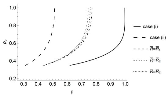
Figure 2. Dependence of ${\rho }_c$ on p for different yield criteria.

In what follows, it is assumed that the disk is loaded with the pressure p₀ = 140 MPa. The effect of the yield criterion on the distribution of stresses has been discussed in [31]. Therefore, the present paper is restricted to evaluating this effect on the distribution of strains.

Figure 3 shows the variation of the principal strains with the dimensionless radius at the end of loading found using the solutions given in Section 4. The distribution of the radial strain is the least sensitive to the choice of the yield criterion (Figure 3c). The distribution of the circumferential strain is more sensitive because of the solution for case (ii) (Figure 3b). The choice of the yield criterion has the most significant effect on the distribution of the axial strain (Figure 3a). The effect is pronounced in the vicinity of the inner radius of the disk.

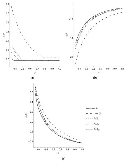
Figure 3. Radial distribution of axial (a), circumferential (b) and radial (c) strains.

The effect of the yield criterion on the distribution of the residual strains found from Equation (52) is shown in Figure 4. It is seen from Figure 3 and Figure 4 that the residual strains are more strongly affected than the strains at the end of loading. In particular, there is a significant deviation of all residual strains for Case (ii) from four other cases. However, the difference in the residual axial strain for the different yield criteria is negligible in the common elastic region (Figure 4a).

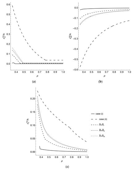
Figure 4. Radial distribution of residual axial (a), circumferential (b) and radial (c) strains.

6. Conclusions

Many metallic materials have different yield stresses in the directions of three principal axes of anisotropy. In the case of a sheet, the different yield stresses in its plane are often replaced with average yield stress independent of the direction. It has been shown in the present paper that this simplification in the theoretical description of material behavior can result in a very significant difference in the distribution of strains and residual strains even in the case of infinitesimal strains. It is expected that this difference will be even more considerable in the case of using the assumption of transversely isotropic yield criteria in the modeling of metal forming processes at large strains.

References

- Rees, D. Basic Engineering Plasticity; Elsevier: Amsterdam, The Netherlands, 2006. [Google Scholar] [CrossRef]
- Banabic, D. Sheet Metal Forming Processes: Constitutive Modeling and Numerical Simulation; Springer: Heidelberg, Germany, 2010. [Google Scholar] [CrossRef]
- Wagoner, R.; Li, M. Simulation of springback: Through-thickness integration. Int. J. Plast. 2007, 23, 345–360. [Google Scholar] [CrossRef]
- Prime, M.B. Amplified effect of mild plastic anisotropy on residual stress and strain anisotropy. Int. J. Solids Struct. 2017, 70–77. [Google Scholar] [CrossRef]
- Essa, S.; Argeso, H. Elastic analysis of variable profile and polar orthotropic FGM rotating disks for a variation function with three parameters. Acta Mech. 2017, 228, 3877–3899. [Google Scholar] [CrossRef]
- Yıldırım, V. Numerical/analytical solutions to the elastic response of arbitrarily functionally graded polar orthotropic rotating discs. J. Braz. Soc. Mech. Sci. Eng. 2018, 40, 320. [Google Scholar] [CrossRef]
- Jeong, W.; Alexandrov, S.; Lang, L. Effect of plastic anisotropy on the distribution of residual stresses and strains in rotating annular disks. Symmetry 2018, 10, 420. [Google Scholar] [CrossRef]
- Wang, C.; Kinzel, G.; Altan, T. Mathematical modeling of plane-strain bending of sheet and plate. J. Mater. Process. Technol. 1993, 39, 279–304. [Google Scholar] [CrossRef]
- Pourboghrat, F.; Chung, K.; Richmond, O. A hybrid membrane/shell method for rapid estimation of Springback in anisotropic sheet metals. J. Appl. Mech. 1998, 65, 671–684. [Google Scholar] [CrossRef]
- Chakrabarty, J.; Bin Lee, R.; Chan, K. An exact solution for the elastic/plastic bending of anisotropic sheet metal under conditions of plane strain. Int. J. Mech. Sci. 2001, 43, 1871–1880. [Google Scholar] [CrossRef]
- Leu, D.-K. Relationship between mechanical properties and geometric parameters to limitation condition of springback based on springback–radius concept in V-die bending process. Int. J. Adv. Manuf. Technol. 2018, 101, 913–926. [Google Scholar] [CrossRef]
- Salimi, M.; Jamshidian, M.; Beheshti, A.; Sadeghi Dolatabadi, A. Bending-unbending analysis of anisotropic sheet under plane strain condition. J. Adv. Mat. Eng. 2008, 26, 77–86. [Google Scholar]
- Li, D.; Luo, Y.; Peng, Y.; Hu, P. The numerical and analytical study on stretch flanging of V-shaped sheet metal. J. Mater. Process. Technol. 2007, 189, 262–267. [Google Scholar] [CrossRef]
- Paul, S.K. Non-linear correlation between uniaxial tensile properties and shear-edge hole expansion ratio. J. Mater. Eng. Perform. 2014, 23, 3610–3619. [Google Scholar] [CrossRef]
- Kim, J.H.; Kwon, Y.J.; Lee, T.; Lee, K.-A.; Kim, H.S.; Lee, C.S. Prediction of hole expansion ratio for various steel sheets based on uniaxial tensile properties. Met. Mater. Int. 2018, 24, 187–194. [Google Scholar] [CrossRef]
- Marciniak, Z.; Kuczyński, K. Limit strains in the processes of stretch-forming sheet metal. Int. J. Mech. Sci. 1967, 9, 609–620. [Google Scholar] [CrossRef]
- Bressan, J.; Williams, J. The use of a shear instability criterion to predict local necking in sheet metal deformation. Int. J. Mech. Sci. 1983, 25, 155–168. [Google Scholar] [CrossRef]
- Bressan, J.D.; Wang, Q.; Simonetto, E.; Ghiotti, A.; Bruschi, S. Formability prediction of Ti6Al4V titanium alloy sheet deformed at room temperature and 600 °C. Int. J. Mater. Form. 2020, 1–15. [Google Scholar] [CrossRef]
- Liao, K.-C.; Pan, J.; Tang, S. Approximate yield criteria for anisotropic porous ductile sheet metals. Mech. Mater. 1997, 26, 213–226. [Google Scholar] [CrossRef]
- Huang, H.-M.; Pan, J.; Tang, S. Failure prediction in anisotropic sheet metals under forming operations with consideration of rotating principal stretch directions. Int. J. Plast. 2000, 16, 611–633. [Google Scholar] [CrossRef]
- Chien, W.Y.; Pan, J.; Tang, S.C. Modified anisotropic Gurson yield criterion for porous ductile sheet metals. J. Eng. Mater. Technol. 2000, 123, 409–416. [Google Scholar] [CrossRef]
- Harikrishna, C.; Davidson, M.J.; Nagaraju, C.; RatnaPrasad, A.V. Effect of lubrication and anisotropy on hardness in the upsetting test. Trans. Indian Inst. Met. 2015, 69, 1449–1457. [Google Scholar] [CrossRef]
- Yang, X.-Y.; Yang, C.; Liang, F.; Zhang, W.-X.; Niu, Y. Influence of normal anisotropy coefficient on no-rivet connection quality. Suxing Gongcheng Xuebao/J. Plast. Eng. 2019, 26, 245–250. [Google Scholar] [CrossRef]
- Uscinowicz, R. Characterization of directional Elastoplastic properties of Al/Cu bimetallic sheet. J. Mater. Eng. Perform. 2019, 28, 1350–1359. [Google Scholar] [CrossRef]
- Ning, B.; Zhao, Z.; Mo, Z.; Wu, H.; Peng, C.; Gong, H. Influence of continuous annealing temperature on mechanical properties and texture of battery shell steel. Metals 2019, 10, 52. [Google Scholar] [CrossRef]
- Moura, A.N.; Ferreira, J.L.; Martins, J.B.R.; De Souza, M.V.; Castro, N.A.; Orlando, M.T.D. Microstructure, crystallographic texture, and stretch-Flangeability of hot-rolled multiphase steel. Steel Res. Int. 2020, 91. [Google Scholar] [CrossRef]
- Lequeu, P.; Jonas, J.J. Modeling of the plastic anisotropy of textured sheet. Met. Mater. Trans. A 1988, 19, 105–120. [Google Scholar] [CrossRef]
- Wang, X.; Cao, L.; Peng, X.; Zhang, J.; Zhuang, L.; Guo, M. Relationship among mechanical properties anisotropy, microstructure and texture in AA 6111 alloy sheets. J. Wuhan Univ. Technol. Sci. Ed. 2016, 31, 648–653. [Google Scholar] [CrossRef]
- Inoue, H.; Takasugi, T. Texture control for improving deep Drawability in rolled and annealed aluminum alloy sheets. Mater. Trans. 2007, 48, 2014–2022. [Google Scholar] [CrossRef]
- Serebryany, V.N.; Pozdnyakova, N.N. Evaluation of the normal anisotropy coefficient in AZ31 alloy sheets. Russ. Met. (Metally) 2009, 2009, 58–64. [Google Scholar] [CrossRef]
- Grechnikov, F.V.; Erisov, Y.A.; Alexandrov, S.E. Effect of the anisotropic yield condition on the predicted distribution of residual stresses in a thin disk. Dokl. Phys. 2019, 64, 233–237. [Google Scholar] [CrossRef]
- Cohen, T.; Masri, R.; Durban, D. Analysis of circular hole expansion with generalized yield criteria. Int. J. Solids Struct. 2009, 46, 3643–3650. [Google Scholar] [CrossRef]
- Hill, R. The Mathematical Theory of Plasticity; Oxford University Press: New York, NY, USA, 1950. [Google Scholar]
- Watson, M.; Dick, R.; Huang, Y.H.; Lockley, A.; Cardoso, R.; Santos, A. Benchmark 1—Failure prediction after cup drawing, reverse redrawing and expansion part A: Benchmark description. J. Phys. Conf. Ser. 2016, 734, 022001. [Google Scholar] [CrossRef]
- Dixit, U.S.; Kamal, S.M.; Shufen, R. Autofrettage Processes: Technology and Modelling; CRC Press: Boka Raton, FL, USA, 2019. [Google Scholar]
Publisher’s Note: MDPI stays neutral with regard to jurisdictional claims in published maps and institutional affiliations. |
© 2020 by the authors. Licensee MDPI, Basel, Switzerland. This article is an open access article distributed under the terms and conditions of the Creative Commons Attribution (CC BY) license (http://creativecommons.org/licenses/by/4.0/).