Solar Irradiance Forecasting Based on Deep Learning Methodologies and Multi-Site Data

Abstract

The ever-growing interest in and requirement for green energy have led to an increased focus on research related to forecasting solar irradiance recently. This study aims to develop forecast models based on deep learning (DL) methodologies and multiple-site data to predict the daily solar irradiance in two locations of India based on the daily solar radiation data obtained from NASA’s POWER project repository over 36 years (1983–2019). The forecast modeling of solar irradiance data is performed for extracting and learning the symmetry latent in data patterns and relationships by the machine learning models and utilizing it to predict future solar data. The goodness of fit and model performance are compared with rolling window evaluation using mean squared error, root-mean-square error and coefficient of determination ($R^2$) for evaluation. The contributions of this study can be summarized as follows: (i) time series models based on deep learning methodologies were implemented to forecast the daily solar irradiance of two locations in India in consideration of the historical data collected by NASA; (ii) the models were developed on the basis of single-location univariate data as well as multiple-location data; (iii) the accuracy, performance and reliability of the model were investigated on the basis of standard performance evaluation metrics and rolling window evaluation; (iv) the feature importance of the nearby locations with respect to forecasting target location solar irradiance was analyzed and compared based on the solar irradiance data obtained from NASA over 36 years. The results indicate that the bidirectional long short-term memory (LSTM) and attention-based LSTM models can be used for forecasting daily solar irradiance data. According to the findings, the multiple-site data with solar irradiance historical data improve upon the forecast performance of single-location univariate solar data.

1. Introduction

1.1. Motivation of the Study

Climate changes in recent times and the high demand for electricity have led to the requirement of power generation from green and renewable sources, solar energy being one of them. Solar energy, which is an abundant sustainable energy resource, causes the least harm to the environment, turning the Sun into a major source of energy [1]. This solar power can be harnessed either through concentrated power plants or photovolatic (PV) power plants. Here, we deal with the PV power plants; their performance is mainly related to the factors of electrical parameters of its components (PV panels, inverters), characteristics of the installation (orientation, tilt angle) and meteorological conditions [2]. The meteorological factor affecting the power produced by a PV field is mainly the absorbed solar irradiance. There is, in fact, a linear correlation between the PV modules’ maximum power and the solar irradiance [3]. The value of this solar irradiance being high or low depends on the geographical location and time along with the orientation of the panel that is relative to both the Sun and the sky [4]. As such, solar power tends to have a chaotic and intermittent behavior. In this study, the aim is to forecast irradiance optimally and in a generalized manner, as we face a problem similar to that of solar power forecasts [5]. The solar irradiance forecasting is performed on historical data from two locations in India for protection of the environment as well as energy security. The main aim is to achieve an increase in the amount of renewable or green energy contribution to the power generated.

1.2. Problem Statement

The PV system is required for the conversion of solar energy to electricity. However, having the environmentally friendly characteristic cannot guarantee the acceptance of PV as an alternative to conventional energy sources. The techno-economical study for viability of any PV system requires accurately estimating the energy yield with an appropriate mathematical model. Different models were proposed for the prediction of PV module performance. However, these models mostly have a complicated structure requiring detailed knowledge of the parameters which are normally unavailable in the manufacturer’s data sheet. Therefore, such models are not suitable for output power calculation. It is the ambient temperature and solar irradiance meteorological data that govern the output of a PV system. Therefore, reliable temperature and radiation data should be readily available for the design of a techno-economically viable photovoltaic system. Because of the difficulties in installation, calibration, maintenance and high cost for measurement of these data, they are either not available or are only partially available at the installation site. Hence, the demand exists for the development of alternative ways to predict them [6,7]. Solar irradiance is also characteristically variable; because of this, competent strategies of forecasting are required for enabling greater penetration of solar power. Influence of location, weather and other meteorological factors also make forecasting solar irradiance a challenging task. Therefore, for successful integration of solar energy with traditional generation supplies, the ability to accurately forecast solar irradiance is essential.

1.3. Related Work

There are basically three types of forecasting techniques: numerical weather prediction, image-based prediction and statistical and machine learning (ML) methods ranging for a period of short-term, medium-term and long-term predictions. Solar irradiance data are time series data, i.e., ranging for a period of time in sequential manner, and traditionally, linear forecasting methods were widely used because they were well understood, easy to compute and provided stable forecasts. Autoregression (AR) [8], the moving-average model (MA), autoregressive with exogeous inputs (ARX) [9], autoregressive moving-average (ARMA) [10], autoregressive moving-average with exogeous inputs (ARMAX) [11], autoregressive integrated moving average (ARIMA) [12], seasonal autoregressive integrated moving average (SARIMA) [13], autoregressive integrated moving-average with exogeous inputs (ARIMAX) [14], seasonal autoregressive integrated moving-average with exogeous inputs (SARIMAX) [15] and generalized autoregressive score (GAS) [16,17] are the traditional forecast models. Belmahdi et al. [18] proposed the ARMA and ARIMA models for forecasting the global solar radiation parameter. The models showed improvement in terms of forecast error; however, only the solar radiation parameter was considered. The geographical or meteorological parameters were not employed. These are mostly linear over the previous inputs or states; hence, they are not adapted to many real-world applications. One major limitation is their pre-assumed linearity form of the data that cannot capture complex nonlinear patterns. The challenges also include lower forecast accuracy and less scalability for big data. Yagli et al. [19] performed a study using satellite-derived irradiance data from multiple locations on 68 machine learning models. The research proposed that multilayer perceptron (MLP) models were one of the best performers and, for assessment of model performance, resulted in a daily or short evaluation period as advised. Following this, the neural network models used here were focused for day-ahead forecasting. The neural network models (NN) work on nonlinear transforming layers with data not required to be necessarily stationary. Neural networks are also strongly capable of determining the complex structures in data, working as an efficient tool for reconstruction of a noisy system driven by data, which is why they are suitable for complex and variable time series forecasting. These are suited for modeling problems which require capturing dependencies and are capable of preserving knowledge as they progress through the subsequent time steps in the data. The authors of [20] proposed an approach for prediction of solar irradiance using deep recurrent neural networks with the aim of improving model complexity and enabling feature extraction of high-level features. The proposed method showed better performance than the conventional feedforward neural networks and support vector machines. The recurrent neural network (RNN) [21] architecture is a special type of neural network accounting for data node dependencies by preserving sequential information in an inner state, which allows the persistence of knowledge accrued from subsequent time steps. However, the RNN is prone to vanishing and exploding gradients. This led to the development of RNN variants such as long short-term memory (LSTM) networks [22], bidirectional LSTM and gated recurrent units (GRU) as extensions of the RNN architecture by replacing the conventional perceptron architecture with memory cell and gating mechanisms that regulate information flow across the network. These variants are widely used for the task of solar irradiance forecasting. The authors of [23] stated that LSTM is a powerful approach for time series forecasting; they used it for day-ahead prediction of solar irradiance. The study proved the LSTM model to be robust; it outperformed other forecast mechanisms such as gradient boosting regression, feedforward neural networks and the persistence model. The authors of [24] proposed a mechanism for hourly day-ahead prediction of solar irradiance using the weather forecasting data. The proposed model consisting of the LSTM variant was compared to the persistence algorithm, linear least square regression and multilayered feedforward neural networks using a backpropagation algorithm (BPNN) for solar irradiance prediction which resulted in LSTM performing the best among all of the methods. The authors of [25] developed a least absolute shrinkage and selection operator (LASSO) and LSTM integrated temporal model for solar intensity forecasting which could predict short-term solar intensity with high precision. Furthermore, recurrent neural networks can be divided into two categories based on the type of mechanism they follow, one being the traditional memory-based models and the other being the attention-based ones. Some of the memory-based models are LSTM, GRU, bidirectional RNNs and so on, while some attention-based models are the attention LSTM, self-attention generative adversarial networks and multi-headed LSTM. The memory-based RNNs are the most widely used models for the task of solar irradiance forecasting in literature. Here, we also intend to introduce the attention mechanism for the task of solar irradiance forecasting. For the task of predicting an element, the attention vector is estimated on the strength of its correlation with other elements and then the sum of these values, which are weighted by the attention vector, is taken. The attention mechanism which was originally introduced and used specifically for machine translation has been recently used for time series forecasting in solar energy tasks. The authors of [26] proposed a temporal attention mechanism for forecasting solar power production from PV plants. The authors of [27] improved upon the attention-based architecture of transformers for forecasting solar power production. In previous works, the prediction task was performed on data from a single target location. The data from the surrounding locations were not exploited for predicting future values of target location. Here, along with the target location’s data, the regional data surrounding the target location were also utilized for building the model. This was done in order to exploit the available data of multiple locations and their contribution in forecasting the future value of a particular target location. A thorough study focusing on various memory-based and attention-based deep recurrent neural network mechanisms for solar irradiance forecasting has not been carried out yet. As such, the DNN-based time series models were built on the basis of the multiple-site concept to forecast the daily solar irradiance of two locations in India on data collected from NASA over a period of 36 years.

1.4. Contributions of the Study

The variable nature of solar energy poses challenges in its integration to the power grid. Accurate forecasting is required for a techno-economically viable solar energy system. The photovoltaic power data are often proprietary and not publicly available, which creates the need to utilize the satellite-derived information of solar irradiance, since the relationship between solar power and solar irradiance is quasilinear [19]. Forecasting at different time horizons has different applications for solar energy systems such as monitoring, maintenance of stability and regulation, management of scheduling and unit commitment. Hence, solar irradiance forecasting is crucial for the domain of solar energy’s advancement in economic feasibility and efficient market penetration; thus, it is essential in order to pave the way for solar energy to be a major type of green energy. The study aims to develop forecast models based on deep learning (DL) methodologies and data from multiple sites to predict the daily solar irradiance. The deep neural network mechanism of machine learning was chosen since the machine-learning-based model estimates particular types of data with high accuracy in comparison to the traditional statistical mechanisms. The machine learning models are capable of extracting and learning the inherent symmetry in patterns and relationships in data. Along with the memory-based variants of RNN, the study also introduces the attention-based mechanism for forecasting solar irradiance. The machine learning models are data-driven, and a large data set is required to understand the behavior of the system, which is often complex. Hence, the past 36 years (1983–2019) of data were provided to the model. For further validation of the proposed mechanism, two locations in India along with the adjoining regional sites were considered for testing the forecast accuracy. The goodness of fit and model performance were compared with rolling window evaluation using mean squared error, root-mean-square error and coefficient of determination ($R^2$) for evaluation. To the best of our knowledge, no comprehensive investigation of solar irradiance forecast models utilizing the RNN variants and multiple-site data has been performed yet. The contributions of this study can be summarized as follows:

• Time series models based on deep learning methodologies were implemented to forecast the daily solar irradiance of two locations in India through consideration of the historical data collected.
• The models were developed on the basis of single-location univariate solar irradiance data as well as data from multiple locations.
• The accuracy, performance and reliability of the model were investigated on the basis of standard performance evaluation metrics and rolling window evaluation.
• The feature importance of the nearby locations with respect to forecasting target location solar irradiance was analyzed and compared on the basis of the solar irradiance data obtained from NASA over 36 years.

The paper is organized as follows: Section 2 highlights the materials and methods considered in this work. The data set used in this study along with the forecast framework, the methodology developed and the metrics used for performance evaluation are discussed in Section 2. The performance of the forecasting models and a discussion are presented in Section 3. The conclusion is given in Section 4.

2. Materials and Methods

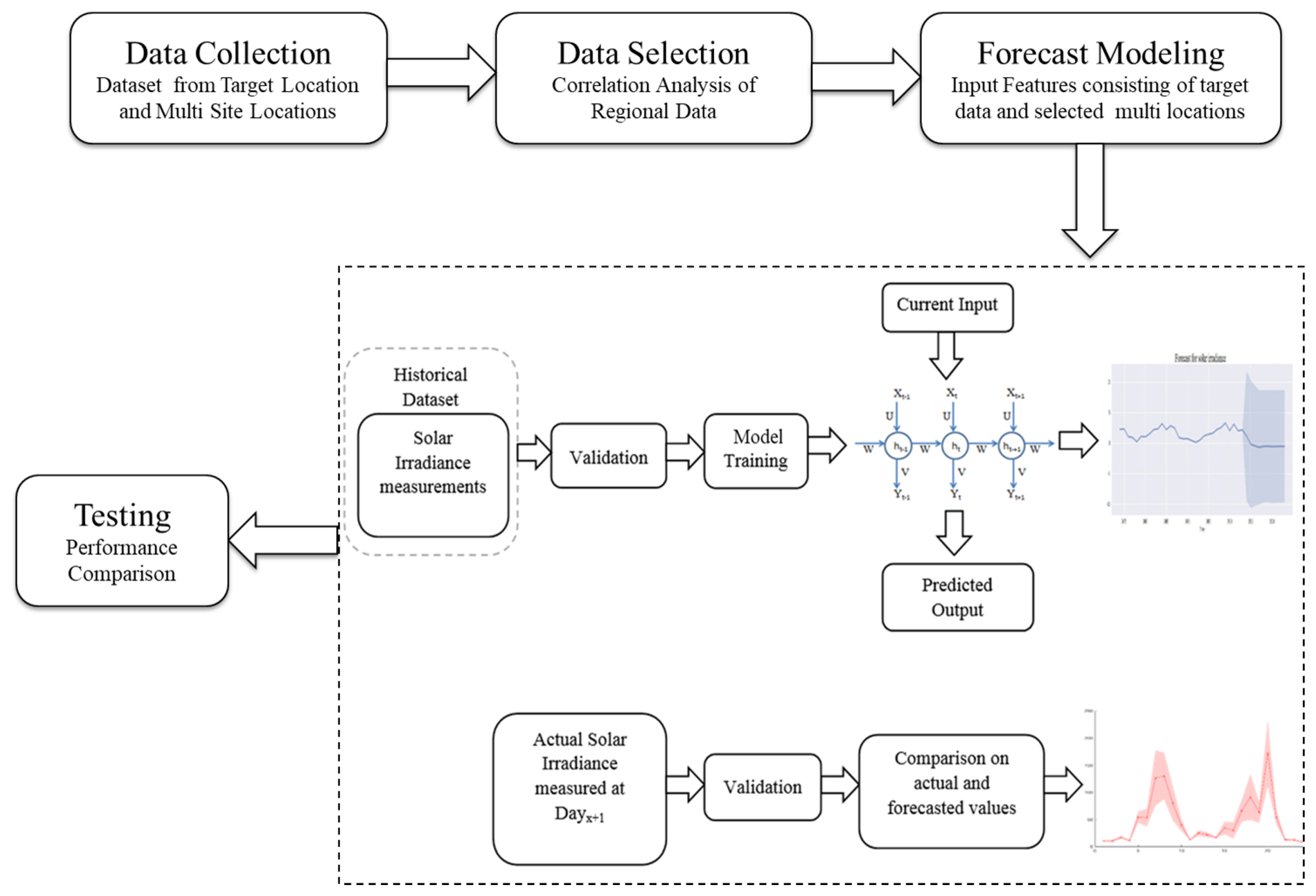
In the sections that follow, the methodology of the proposed deep learning framework for forecasting daily solar irradiance is discussed. The outline of the proposed framework is shown in Figure 1. The first step consisted of data collection of the point target location and the multiple-site region surrounding the target location. Then, the proposed model selected the relevant location data from the multiple-site high-dimensional data. The optimal model of forecasting was then obtained utilizing deep learning models. The proposed mechanism was validated on meteorological data from two target locations for different time horizons of forecasting. The efficiency was compared with the single-location forecast model and various deep learning models in terms of performance metrics.

2.1. Data Collection

Forecast models for solar irradiance were built on historical time series data. These data can be obtained through ground-based stations or satellite-based data sets. Due to the limited availability of ground-based stations, the satellite-based data was utilized here from NASA’s POWER database, which is open access with long-term coverage. The daily solar irradiance data consisting of solar radiation incidents on a horizontal surface having unit kwhr/m${}^2$ per day were collected from the SSE-Renewable Energy Community of the POWER Data Access Viewer for a period of 36 years from 1983 to 2019.

The problem of forecasting that we are trying to address here is the forecast of data in a particular target location utilizing not only the target location data, but also the data of the region surrounding the target location. This would address the data dependency on unrelated features, since it is only the solar irradiance data that is considered for all of the sites. Instead of only relying on lags of the particular target locations data, which might consist of discrepancies, this framework considered multiple-site data of the target solar irradiance feature. The relevance of the feature is discussed in the next section. Here, we introduce a multi-site mechanism converting the problem into multivariate forecasting utilizing the concerned solar irradiance data from multiple sites. Figure 2 and Figure 3 below show the point location and the region selected for the solar irradiance data from the POWER Regional Data Access widget which provides access to near real-time data. Point P represents the target location while the enclosed region represents the multiple sites surrounding the target location. These regional data were further analyzed and processed in the next step for the task of forecasting. For a single point—that is, the target location’s data—a near real-time $1/2\times 1/2$ degree data set was accessed by supplying a numeric vector with length of two, giving the decimal degree longitude and latitude in that order for data to download. For the regional coverage, a bounding box was attained for the surrounding location to a target point location with a maximum bounding box of $4.5\times 4.5$ degrees of $1/2\times 1/2$ degree data with 100 data points maximum in total. A numeric vector with length of four, as latitude and longitude coordinates of the lower left and upper right, was provided to attain the enclosed area. These coordinates of the data set utilized for the case study are represented in

Table 1. Data set description for target location and regional data.

Location #	Target Location Coordinates	Number of Enclosed Regional Sites	Enclosed Site Coordinates
1	23.25991, 77.41261	12	23.9645, 78.2255; 22.7947, 76.5556
2	22.71961, 75.85771	15	23.4011, 76.7314; 22.1450, 74.9077

.

Table 2. Descriptive statistics for daily solar irradiance.

Statistic	Value for Location 1	Value for Location 2
Total Observations	13,000	13,000
Date Range	1983–2019	1983–2019
Minimum	0.2	0.16
Maximum	8.41	8.66
Mean	5.09	5.17
Standard Deviation	1.42	1.38

lists the descriptive statistics of the target solar irradiance data.

2.2. Data Selection

The data of 36 years were collected for the target location as well as the enclosed region. As it can observed from Table 1, the data collected for forecasting Location 1 and 2 consisted of 12 and 15 sites, respectively. However, the sites surrounding the target location may not all have been correlated and helpful in forecasting solar irradiance data. The dimensions of the features needed to be reduced to utilize only the relevant features for forecast purpose. Here, feature implies the solar irradiance data of all of the locations as depicted in Table 1. Therefore, the forecast framework further consisted of analyzing the correlation and feature importance of the multiple-site data for forecasting the target location data. This task was accomplished by utilizing the Pearson, Spearman and XGBoost Ranking as discussed below.

2.2.1. Pearson Correlation

Pearson correlation measures the linear relationship between related variables. −1 implies the variables are negatively correlated, 0 denotes they are not correlated and 1 means they are perfectly correlated. It generally measures the global synchrony.

$$Cor{r}_{xy}=\frac{n\sum x_i{y}_i-\sum x_i\sum y_i}{\sqrt{n\sum x_i^2-{(\sum x_i)}^2}\sqrt{n\sum y_i^2-{(\sum y_i)}^2}}$$

(1)

2.2.2. Spearman Correlation

Spearman correlation is a correlation test which is nonparametric in nature. It does not carry assumptions regarding the distribution of the data and is the appropriate correlation analysis when the variables are measured on a scale. Equation (2) denotes the formula for calculation of Spearman correlation with n number of observations and $d_i$ being the difference between ranks of the corresponding variables.

$$Corr=1-\frac{6\sum d_i^2}{n(n^2-1)}$$

(2)

2.2.3. XGBoost

Along with the correlations between target and neighboring locations, we also computed the feature importance of the solar irradiance values. eXtreme Gradient Boosting (XGBoost) utilizes information gain for estimating the importance of feature. After the boosted trees are constructed, the importance scores for each attribute can be retrieved in a straightforward manner. This importance is calculated for all of the features which ranks and compares them to each other. Calculation of feature importance is performed for a single decision tree. This is done by the amount in which each split point contributes to the improvement of the performance measure, weighted by the number of observations the node is responsible for. The performance is measured using an error function and feature importance calculated by the average across all of the decision trees within the model.

These scores would indicate the relation of the multiple sites and the target location, such that only the relevant sites are chosen which would improve the forecast accuracy. Figure 4 depicts the process of selection of m locations from the collected n sites data. The solar irradiance of these m locations and the target location were used for the forecast methodology, utilizing deep neural networks as stated in the next section.

2.3. Forecast Methodology

This section introduces the deep learning methodology of recurrent neural networks and their variants. The vanilla LSTM, GRU, bidirectional LSTM, CNN LSTM and the attention mechanisms are presented below. The networks took the past solar irradiance data of the target location and the selected multi-site locations as input features. The final output $y_{(t-1+\Delta )}$ was the forecast result of future solar data of the target location. Given daily solar irradiance time series X, with $x_i$ representing observed value at time i, $X=\{x_1,x_2,\dots .,x_{(t-1)}\}$, the problem was forecasting $x_{(t-1+\Delta )}$ with $\Delta$ as the horizon w.r.t. different tasks. $y_{(t-1+\Delta )}$ is the prediction with $y_{(t-1+\Delta )}^{{}^{\prime }}=x_{(t-1+\Delta )}$ being the ground-truth value. For every task, $\{x_{(t-w)},x_{(t-w+1)},\dots ,x_{(t-1)}\}$ is used to predict $x_{(t-1+\Delta )}$, where w is the window size because of the assumption that there exists no useful information before the window and the input is fixed. Equation (3) denotes the problem with y representing $\Delta$ days-ahead forecasting of solar irradiance data with deep neural network model f on past historical data. Since data from multiple locations were used, the input data x consisted of time-lagged values of target location data as well as the regional multi-site data.

$$y_{(t-1+\Delta )}=f(x_{(t-w)},x_{(t-w+1)},\dots ,x_{(t-1)})$$

(3)

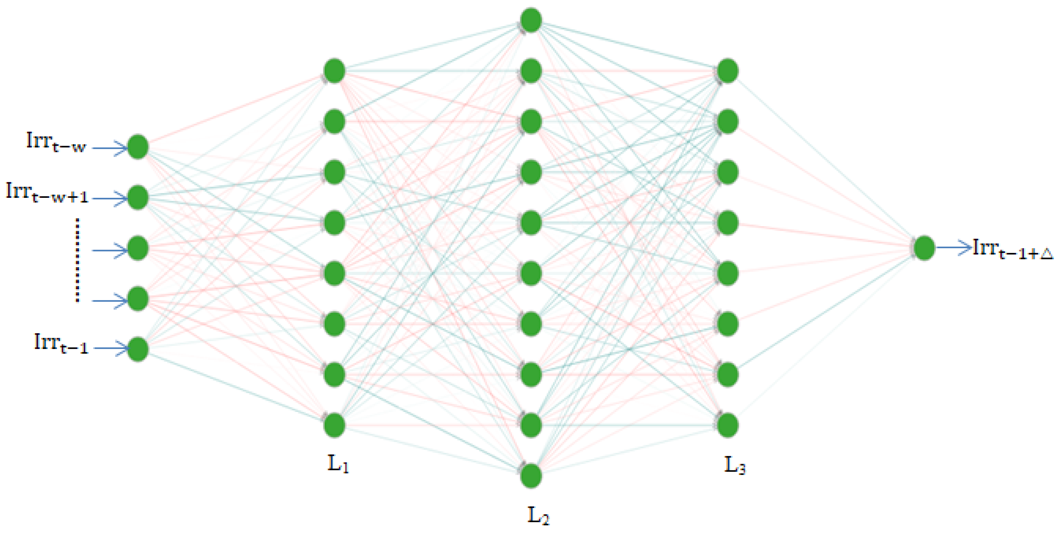
The solar irradiance forecast modeling in the univariate scenario for a single location was performed by taking the historical data at time $t-1+\Delta$, denoted by $Ir{r}_{(t-1+\Delta )}$ in Figure 5, as the target variable and the window-lagged data, $Ir{r}_{(t-w)},Ir{r}_{(t-w+1)},\dots Ir{r}_{(t-1)}$, as input variables. w represents the window length for the lagged time series, which was decided upon using the autocorrelation and partial autocorrelation characteristics of the data. $L_i$ represents the ith hidden layer L, in which the i values are set during model tuning. Overall, the future values of solar irradiance were predicted using the past and present values according to set window size.

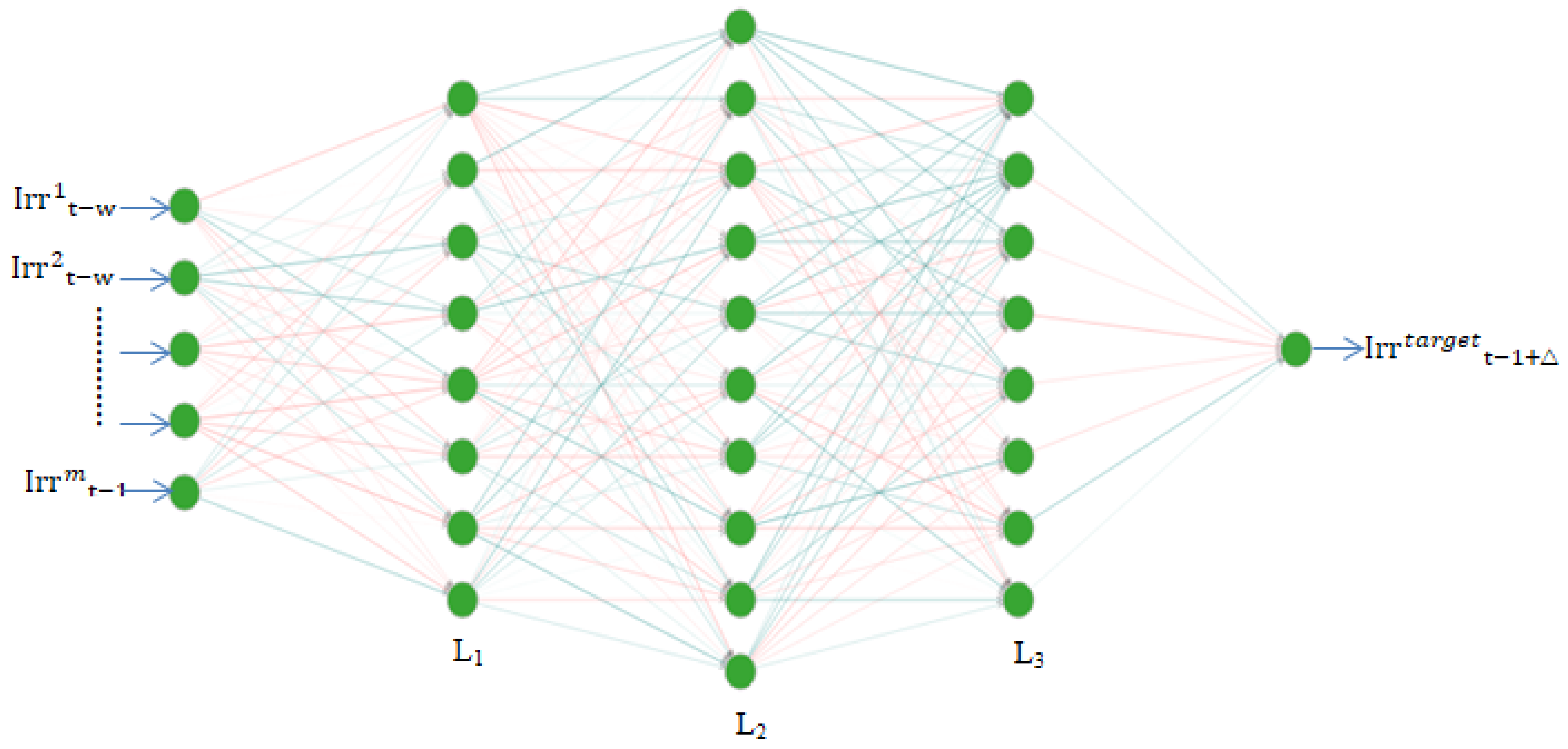
In the proposed forecast framework, the difference was in the features utilized for future value prediction. Instead of only depending upon the past lagged values of one location, the values of multiple locations were utilized. This converted the univariate form of forecasting into a multivariate form with solar irradiance data from the target location as well as m locations as features. The final aim was forecasting solar irradiance values for the target location. Figure 6 represents this framework, with $Ir{r}^j$ representing jth location data, where j ranges from 1 to m and $Ir{r}^{target}$ denoting solar irradiance for target location.

The deep neural network assigns weights to the past input data in order to predict the future values. The recurrent neural network variant of DNN is used for the task of time series forecasting since it is suited for sequential data and remembers the temporal dependencies in data. Equation (4) represents a vanilla RNN which takes into account the present input along with the output of the previous state. The proposed framework utilizes the enhanced cell mechanism of this vanilla RNN which is capable of understanding more complex and long-term dependencies.

$$y_t=W_{XH}{X}_t+W_{HH}{H}_{t-1}$$

(4)

2.3.1. LSTM

LSTM belongs to the family of recurrent neural networks, improving on the efficiency of traditional sequence learning mechanisms. The problem of vanishing and exploding gradients persists in the RNN, which led to the development of LSTM in order to overcome these problems of RNNs.

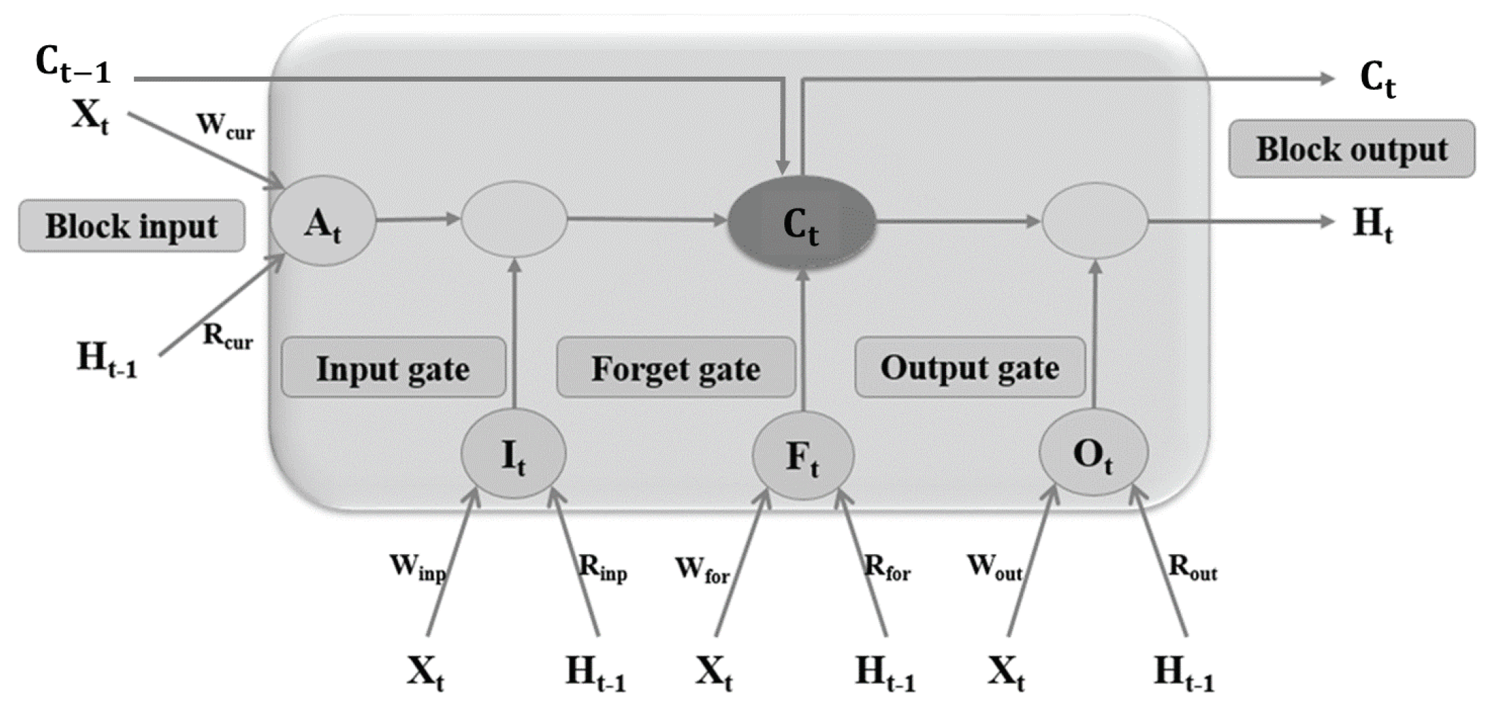
LSTM, as shown in Figure 7 [28], introduces additional computation components to the RNN, the input gate, the forget gate and the output gate. The equations for the forward pass are stated below:

$$\begin{array}{c}\hfill A_t=tanh(W_{cur}{X}_t+R_{cur}{H}_{t-1})\\ \hfill I_t=\sigma (W_{inp}{X}_t+R_{inp}{H}_{t-1})\\ \hfill F_t=\sigma (W_{for}{X}_t+R_{for}{H}_{t-1})\\ \hfill O_t=\sigma (W_{out}{X}_t+R_{out}{H}_{t-1})\\ \hfill C_t=I_t\odot A_t+F_t\odot C_{t-1}\\ \hfill H_t=O_t\odot tanh\left(C_t\right)\end{array}$$

(5)

The current input and the previous state are processed by $A_t$ after which the input gate $I_t$ decides upon the parts of $A_t$ to be added in the long-term state $C_t$. $F_t$ is the forget gate with the responsibility of deciding which parts of $C_{t-1}$ are to be erased, discarding the unnecessary parts. The output gate $O_t$ finds the parts of $C_t$ to be read and shown as output. As such, there exists a short-term state $H_t$ that is shared between the cells and a long-term state $C_t$ in which the memories are dropped and added by the respective gates. Weight updation is carried out by following equation below with * denoting any one among {cur,inp,for,out} and $<\ast ,\ast >$ denoting the product.:

$$\begin{array}{c}\hfill \begin{array}{c}\hfill \delta W_{\ast }=\sum _{t=0}^T<{\delta }_{\ast t},X_t>\\ \hfill \delta R_{\ast }=\sum _{t=0}^{T-1}<{\delta }_{\ast t+1},H_t>\end{array}\end{array}$$

(6)

2.3.2. Bidirectional LSTM

LSTM processes the inputs in strict temporal order. This indicates that the current input has context of previous inputs, but not the future. The bidirectional LSTM [29] model was introduced to address this shortcoming. It duplicates the LSTM processing chain so that the inputs are processed in both forward and reverse time order. This allows the network to look into the future context as well.

2.3.3. GRU

The gated recurrent unit [30] can be viewed as the simplified version of LSTM in which the cell states are not used explicitly. The main simplification made is that both the state vectors are merged into a single vector. Figure 8 [31] represents a GRU cell, and the equations followed during forward pass are shown below.

$$\begin{array}{c}\hfill z_t=\sigma (W_{xz}{x}_t+W_{hz}{h}_{t-1})\\ \hfill r_t=\sigma (W_{xr}{x}_t+W_{hr}{h}_{t-1})\\ \hfill g_t=tanh(W_{xg}{x}_t+W_{hg}(r_t\otimes h_{t-1})\\ \hfill h_t=(1-z_t)\otimes tanh(W_{xg}{h}_{t-1}+z_t\otimes g_t)\end{array}$$

(7)

There exists a single gate controller which controls the input gate and the forget gate. On a gate controller giving an output of 1, the input gate is opened while the forget gate is closed, and vice versa when the output is 0. This implies that on requirement of a memory to be stored, the location to be stored is erased first. It is, in fact, a variant of LSTM which is used frequently. No output gate exists and the full state vector is output every time step. However, there is a new gate controller which controls the part of the previous state which will be shown to the main layer.

2.3.4. CNN LSTM

CNN [32] architecture consists of three types of layers: the convolutional layer, the pooling layer and the fully connected layer. Convolutional layers take in the feature maps as inputs from the previous layer and perform convolution operations between filters and the inputs.

$$conv(x,y)=\sum _i{w}_i{v}_i$$

(8)

where $w_i$ are the convolutional kernel parameters, $v_i$ the output of previous layer and $(x,y)$ the spatial coordinate. A complete feature map is obtained as follows with b as scalar bias and g as the nonlinear activation function.

$$z(x,y)=g\left(conv\right(x,y)+b)$$

(9)

The hybrid CNN LSTM method consists of a series of connections between the convolutional and LSTM layers. The convolution operation reduces the number of parameters and uses a pooling layer for combining the output of a cluster of neurons to a single neuron. The pooling layer also reduces parameters and computation cost of the network. Max pooling is used here which selects the maximum value from neuron clusters. The LSTM layers are placed after the CNN layers. The past and future contexts are kept in view along with consolidation of memory units and cell states for the temporal dependencies. The vanishing and exploding gradients are also addressed by the LSTM layers. The dropout regularization is used for overfitting as well.

2.3.5. Attention LSTM

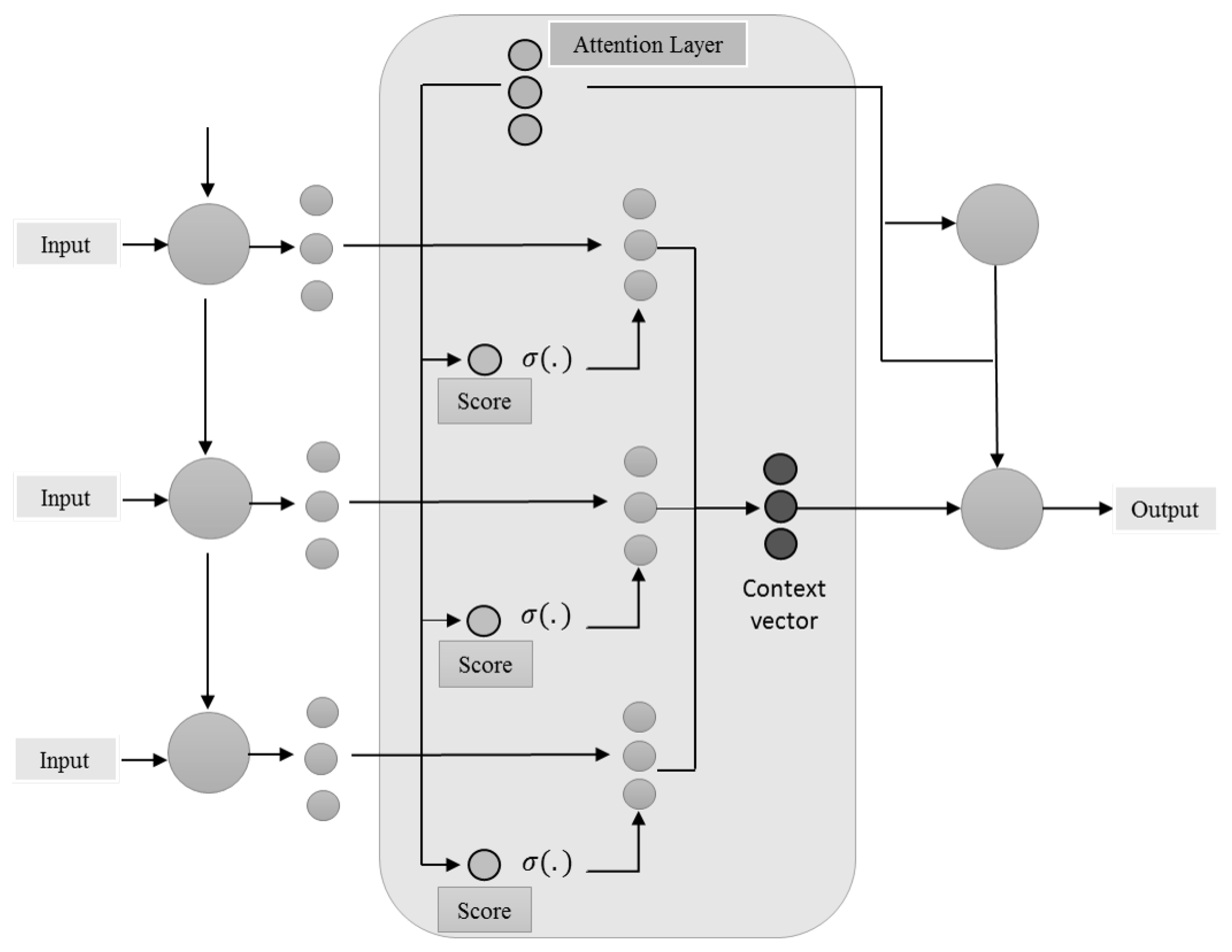
The attention mechanism belongs to the sequence-to-sequence model which was built mainly for neural machine translation. It consists of an encoder and decoder with encoder encoding the input to a fixed length vector and decoder translating it [33]. The attention mechanism addresses the long-term dependencies in which past values from far back might be affecting the present day forecast. The identification of relevant features and dynamic interdependencies can be done through attention. The attention mechanisms mainly differ in the architecture of the encoder-decoder adopted and the score function. In the sequence-to-sequence model, the decoder receives the last encoder hidden state from the encoder, a vector representation, much like an input sequence’s numerical summary. Thus, for a long input, the decoder uses just this one vector representation to output the prediction, which leads to forgetting. As such, attention was introduced, which acts as an interface in between the encoder and decoder providing information from every encoder hidden state to the decoder. As shown in Figure 9 [34], this enables the model to selectively focus on useful parts of the input sequence based on the scoring function, and thus learn the alignment between them.

Here, score represents a typical scoring function which represents the relevance between the input vectors. The whole process is done for computation of the context vector which is then forwarded to the decoder layer [26].

$$score(h_{t-1},s_{t-1})=v_a^{T}tanh(W_a[h_{t-1};s_t]+W_{x}x+b_a)$$

(10)

$${\alpha }_{t-1}=\frac{exp\left(score(h_{t-1},s_{t-1})\right)}{{\sum }_{i=1}^{t}exp\left(score(h_{i-1},s_{i-1})\right)}$$

(11)

$$ContextVector=\sum _{i=1}^t{\alpha }_i{h}_i$$

(12)

where x is the given input, h_t-1 is the hidden state and s_t-1 the cell state. W_a, W_x and b_a are the attention weights and bias. As it can be observed from Figure 9, after the input layer, there exists an encoder layer which processes the input and then forwards it to the attention layer. The $\sigma$ represents the softmax function performed on the score. This attention layer proceeds with the input according to the equations as stated above and then feeds its output to the decoder to be sent to the output layer. Now, these encoder and decoder layers are nothing but the DNN hidden nodes and layers which perform a typical sequential learning from the complete process. The additional benefit is the computation of relevant information after extracting it through the scoring function. This aides in managing long-term dependencies by just the introduction of an attention layer.

In the attention LSTM developed for solar irradiance forecasting, the score function adopted is the content-based attention. The attention vectors in content-based attention [35] or cosine scoring are created on the basis of similarity between the key and memory rows. It computes the cosine similarity which is then normalized by the softmax function.

$$score(s_t,hi)=cosine[s_t,h_i]$$

(13)

The encoder layer consists of the bidirectional LSTM and vanilla LSTM. The hidden outputs from this layer is then fed to the attention layer which computes the score function and then the context vector. This is then forwarded to the decoding fully connected layer or the dense layer which then gives the output that is the forecast values of solar irradiance.

2.4. Performance Evaluation Metrics

In order to verify the performance of forecasting models, the goodness of fit needs to be measured. The common metrics which are used to calculate this include MSE, MAE, RMSE, SSE, $R^2$ score, etc. Here, we use the following metrics as in

Table 3. Forecast performance evaluation metrics.

Metric	Equation
MSE	$\frac{1}{N}{\sum }_{n=1}^N{(E(D_n\mid \overrightarrow{X_n})-F(\overrightarrow{X_n},\overrightarrow{w}))}^2$
RMSE	$\sqrt{\frac{1}{N}{\sum }_{n=1}^N{(E(D_n\mid \overrightarrow{X_n})-F(\overrightarrow{X_n},\overrightarrow{w}))}^2}$
$R^2$	$1-\frac{{\sum }_{n=1}^N{(E(D_n\mid \overrightarrow{X_n})-F(\overrightarrow{X_n},\overrightarrow{w}))}^2}{{\sum }_{n=1}^N{(E(D_n\mid \overrightarrow{X_n})-\overrightarrow{F}(\overrightarrow{X_n},\overrightarrow{w}))}^2}$

. E denotes the expected value or the actual value of the target output and F denotes the output of the forecast model given input X and weight w. MSE and RMSE provide an insight regarding the error. Low values of MSE and RMSE denote better performance. $R^2$ is the coefficient of determination indicating closeness of fit with baseline model. When the $R^2$ score value tends to 1, the relationship between the predictors and response variable is considered to be strong, whereas an $R^2$ score close to 0 indicate the opposite.

3. Results and Discussion

The results of the simulation experiments performed on historical data are presented in this section. The analysis was performed based on test results, which were further analyzed for their diversity, robustness, importance of the features used and the significance of multiple horizons. These results are discussed and represented in the subsections that follow.

3.1. Test Results

The results of the proposed multi-site deep learning forecast methodology were compared with those of the traditional deep learning forecast mechanism for the two locations in India.

Table 4. Forecast performance of Location 1 data set for horizon length of 1.

Model	Single-Location			Multi-Location
	MSE	RMSE	${\mathit{R}}^2$	MSE	RMSE	${\mathit{R}}^2$
LSTM	9.721	9.859	68.62	9.581	9.788	69.06
GRU	9.825	9.912	68.28	9.193	9.588	70.32
CNN	9.714	9.856	68.64	9.213	9.598	70.25
Bidir	9.617	9.806	68.95	9.094	9.536	70.64
Attention	9.610	9.803	68.97	9.399	9.695	69.65

,

Table 5. Forecast performance of Location 1 data set for horizon length of 4.

Model	Single-Location			Multi-Location
	MSE	RMSE	${\mathit{R}}^2$	MSE	RMSE	${\mathit{R}}^2$
LSTM	13.19	11.48	57.41	12.79	11.31	58.68
GRU	13.28	11.52	57.13	12.93	11.37	58.23
CNN	13.22	11.50	57.31	12.94	11.37	58.23
Bidir	13.20	11.49	57.36	12.78	11.30	58.74
Attention	13.21	11.49	57.34	12.69	11.26	59.01

,

Table 6. Forecast performance of Location 1 data set for horizon length of 10.

Model	Single-Location			Multi-Location
	MSE	RMSE	${\mathit{R}}^2$	MSE	RMSE	${\mathit{R}}^2$
LSTM	15.48	12.44	50.24	15.19	12.33	50.98
GRU	15.41	12.41	50.50	16.25	12.75	47.57
CNN	15.05	12.26	51.66	18.37	13.55	40.75
Bidir	15.16	12.31	51.28	14.84	12.18	52.12
Attention	15.23	12.34	51.05	14.38	11.99	53.56

,

Table 7. Forecast performance of Location 2 data set for horizon length of 1.

Model	Single-Location			Multi-Location
	MSE	RMSE	${\mathit{R}}^2$	MSE	RMSE	${\mathit{R}}^2$
LSTM	7.911	8.894	72.29	7.678	8.762	73.11
GRU	7.869	8.871	72.44	8.106	9.003	71.61
CNN	7.937	8.909	72.21	8.317	9.120	70.86
Bidir	7.794	8.828	72.71	7.610	8.724	73.34
Attention	7.866	8.869	72.45	7.631	8.735	73.27

,

Table 8. Forecast performance of Location 2 data set for horizon length of 4.

Model	Single-Location			Multi-Location
	MSE	RMSE	${\mathit{R}}^2$	MSE	RMSE	${\mathit{R}}^2$
LSTM	10.63	10.31	62.75	10.50	10.27	63.06
GRU	10.56	10.27	63.01	10.67	10.33	62.64
CNN	10.68	10.34	62.57	10.93	10.45	61.72
Bidir	10.76	10.37	62.30	10.50	10.25	63.21
Attention	10.79	10.38	62.21	10.69	10.34	62.55

and

Table 9. Forecast performance of Location 2 data set for horizon length of 10.

Model	Single-Location			Multi-Location
	MSE	RMSE	${\mathit{R}}^2$	MSE	RMSE	${\mathit{R}}^2$
LSTM	12.51	11.18	56.34	12.61	11.23	55.89
GRU	13.07	11.43	54.38	12.98	11.39	54.59
CNN	13.40	11.57	53.25	15.12	12.29	47.11
Bidir	12.83	11.32	55.23	12.54	11.19	56.14
Attention	12.65	11.25	55.84	12.45	11.16	56.44

show the performance of the forecasting models in terms of MSE, RMSE and coefficient of determination. The best performing models are shown in bold. For suitability of representation, the MSE values were multiplied by ${10}^3$ and the RMSE values were multiplied by ${10}^2$.

Table 4, Table 5 and Table 6 indicate the performance metrics of each developed model for Location 1 with different horizons. The developed forecast methodology had the lowest MSE and RMSE and the highest $R^2$ score in all of the cases. The bidirectional LSTM performed the best for 1-day-ahead forecasting. However, the attention LSTM proved its superiority in 4-days-ahead and 10-days-ahead forecasting of solar irradiance. The single-location forecast models also performed well; however, the developed multi-location model performed better, indicating its ability to accurately forecast solar irradiance data.

Similar results were observed for Location 2 as represented in Table 7, Table 8 and Table 9. The proposed methodology performed the best among the models compared. The bidirectional LSTM performed the best for forecasting 1-day-ahead and 4-days-ahead solar irradiance, while the attention LSTM outperformed others in forecasting 10-days-ahead data. It was also observed that Location 2 showed the lowest errors, followed by the higher error values of Location 1. The performance of the deep learning forecast methodology was improved by the addition of multiple-site solar irradiance feature.

The tables indicate that the proposed methodology outperformed other models on all data sets, metrics and horizons. The superiority of the multi-site deep learning forecast methodologies was demonstrated by the results obtained through simulations. Furthermore, the bidirectional LSTM and attention-based LSTM models performed the best among other DL models. The bidirectional LSTM models showed their capability of exploiting data from temporal contexts while attention LSTM utilized complex and nonlinear interdependencies between time steps and time series for predicting future values of solar irradiance data. Both of the models showed consistent performance of lower MSE and RMSE values and higher coefficients of determination, with the attention-based models performing the best in longer horizons with more complex characteristics. It can be established that the attention LSTM, based on the content-based scoring function and proposed multi-site data, is indeed an enhancement to the previously developed forecast models.

3.2. Analysis of Diversity and Robustness

As stated by [36], forecasting performed from a single origin tends to be prone to corruption because of occurrences which are unique to that origin. It has also been rightly said that the performance on data outside that used in its construction remains the touchstone for its utility in all applications. Predictive machine learning includes the routine application of repeated subsampling of the data set on which some algorithm is parameterized, which in turn leads to diversity in data rather than in the algorithm [37]. This technique also assesses how well our algorithm would perform in the case of unseen or independent data sets. In the performance estimation model considered here, the model is updated only with new data. Past trained data is not considered from the origin for training again as shown in Figure 10.

The forecast operation was performed not only for 1-day-ahead solar irradiance but also for multiple horizons as indicated in Figure 11. The historical daily solar irradiance data were utilized to forecast 1-day-ahead, 4-days-ahead and 10-days-ahead target data. This also proved the robustness of the proposed methodology for diverse horizons.

Table 4, Table 5, Table 6, Table 7, Table 8 and Table 9 in the previous subsection indicate the results of this performance estimation model for multiple horizons. The error metrics indicate the suitability and reliability of the proposed method for accurately forecasting solar irradiance data.

3.3. Feature Importance Analysis

Selection of features is an important task for DNN models for eliminating features which are not important in forecasting target data and for reducing computational time and complexity. The proposed methodology utilized solar irradiance data from multiple locations for forecasting target solar data. As such, for efficiently selecting the most influential input features, the importance of each variable was determined. This data selection was done by the analysis that was carried out for selection of particular regional point locations from multiple points surrounding the target location.

Table 10. Multi-location feature importance corresponding target solar irradiance for Location 1.

Function	1	2	4	5	8
Pearson	87.4959	90.5483	87.2493	91.7756	91.9108
Spearman	88.9031	91.3695	88.2469	92.2826	92.3385
XGBoost	0.3709	21.3245	0.1822	34.5608	43.5614

and

Table 11. Multi-location feature importance corresponding target solar irradiance for Location 2.

Function	1	4	11	12	14
Pearson	92.5453	91.9138	86.2631	91.2246	87.3032
Spearman	92.5622	91.9727	87.4589	91.7827	88.6667
XGBoost	37.8932	41.0277	0.3307	20.4562	0.2919

show the feature importance on the basis of Pearson, Spearman and XGBoost scoring for both of the locations, respectively. The feature importance was calculated for site IDs 1, 2, 4, 5 and 8 for Location 1, while for Location 2, the sites with IDs 1, 4, 11, 12 and 14 were analyzed. The sites for both of the locations were different and did not overlap with each other. The values of the scores were multiplied by ${10}^2$ for ease of representation. For Location 1, the sites corresponding to number 2, 5 and 8 out of the five sites showed the greatest correlation. In the case of Location 2, site numbers 1, 4 and 12 had the greatest importance out of all five sites. As such, only the most important sites’ solar irradiance data were selected under data selection.

3.4. Comparison for Different Horizons

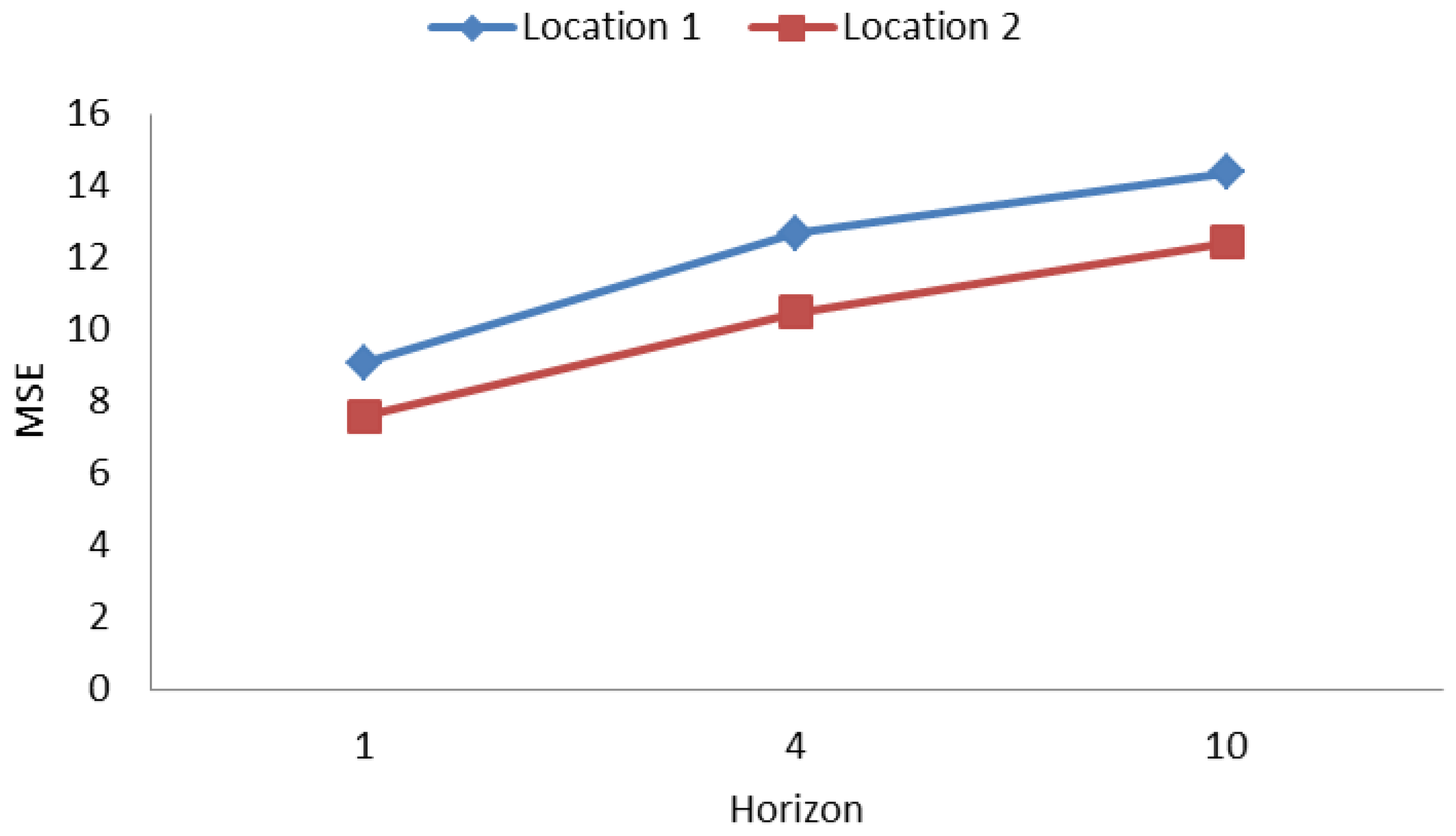
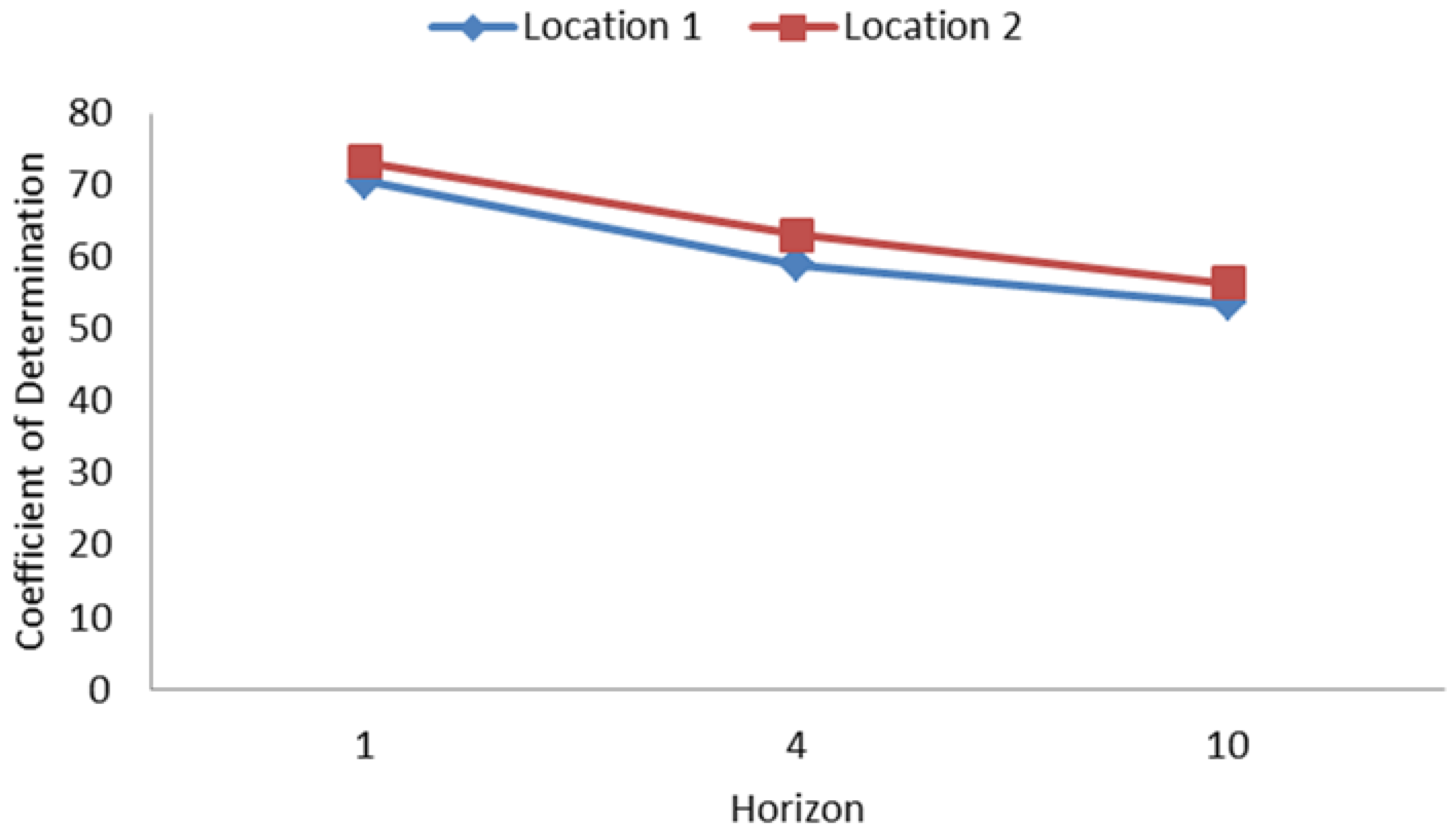
The results also showed the performance of the models for different horizons. As the length of the horizon increased, the performance of the model differed in a similar fashion in all of the cases. The change in performance of the proposed model for both of the locations was observed as the horizon increased. The performance metrics showed similar trends with better performance in shorter horizons. Figure A1 and Figure A2 in Appendix A represents this change for both the locations in terms of MSE and $R^2$ score as the forecast horizon increases. For a horizon length of 1, the models tended to give the best performance metrics. The proposed model again performed the best as compared to the other models. A similar trend was seen for all of the horizon lengths.

4. Conclusions

Solar irradiance forecast has captured the attention of current research due to the requirement and interest in renewable and green energy. Accurate forecasting of solar irradiance is required to understand the solar energy perspective of a region, considering the opportunities as well as challenges related to forecasting. The DNN models can efficiently and accurately predict daily solar irradiance data. In this work, the DNN models were used to predict the daily solar irradiance data with multiple sites data of solar irradiance from two locations in India. A historical data set of solar irradiance over the past 36 years was used for training and testing to accurately forecast solar irradiance in this study. For checking the validation and stability of the simulation results, the goodness of fit of the model was tested using MSE, RMSE and coefficient of determination. The results demonstrated the capability of the proposed methodology in providing accurate daily prediction of solar irradiance. The coefficient of determination ($R^2$) was equal to 70% and 73% for both the locations, respectively. The $R^2$ scores greater than 50 indicated excellent forecast performance of the model. Moreover, the feature importance was analyzed utilizing correlation and XGBoost scores. The results supported the selection of the multi-site data and its goodness of fit. In addition, a comparison of the DNN models on the basis of multiple horizons was also conducted. The results showed that forecasting tasks of shorter horizons shows better accuracy while longer horizons require more complex models.

The present study also exhibited certain limitations. The black box nature of machine learning models make understanding the model difficult. Our future work will concentrate on exploiting the hybrid models consisting of linear and nonlinear models. The limitations of using single models in processing data patterns and the nonstationary behavior of solar irradiance and meteorological parameters in various atmospheric conditions have led to the introduction of hybrid approaches to achieve more accurate results for modeling and forecasting [38,39], which led to enhancement of model interpretability and accuracy. The study considered the data of two locations from a single country. Future research would include target data from multiple locations and different climate zones. In general, promising models with boosted forecast precision can estimate potential solar energy—in particular locations and advance the sustainable planning of solar power applications.

References

1. Heng, J.; Wang, J.; Xiao, L.; Lu, H. Research and application of a combined model based on frequent pattern growth algorithm and multi-objective optimization for solar radiation forecasting. Appl. Energy 2017, 208, 845–866. [Google Scholar] [CrossRef]
2. Amrouche, B.; Le Pivert, X. Artificial neural network based daily local forecasting for global solar radiation. Appl. Energy 2014, 130, 333–341. [Google Scholar] [CrossRef]
3. Amrouche, B.; Sicot, L.; Guessoum, A.; Belhamel, M. Experimental analysis of the maximum power point’s properties for four photovoltaic modules from different technologies: Monocrystalline and polycrystalline silicon, CIS and CdTe. Sol. Energy Mater. Sol. Cells 2013. [Google Scholar] [CrossRef]
4. Lubitz, W. Effect of manual tilt adjustments on incident irradiance on fixed and tracking solar panels. Appl. Energy 2011, 88, 1710–1719. [Google Scholar] [CrossRef]
5. Su, Y.; Chan, L.; Shu, L.; Tsui, K. Real-time prediction models for output power and efficiency of grid-connected solar photovoltaic systems. Appl. Energy 2012, 93, 319–326. [Google Scholar] [CrossRef]
6. Thapar, V.; Agnihotri, G.; Sethi, V.K. Estimation of Hourly Temperature at a Site and its Impact on Energy Yield of a PV Module. Int. J. Green Energy 2012, 9, 553–572. [Google Scholar] [CrossRef]
7. Thapar, V. A revisit to solar radiation estimations using sunshine duration: Analysis of impact of these estimations on energy yield of a PV generating system. Energy Sources Part A Recovery Util. Environ. Eff. 2019, 1–25. [Google Scholar] [CrossRef]
8. Tsay, R.S. Analysis of Financial Time Series Second Edition; John Wiley & Sons: New York, NY, USA, 2005. [Google Scholar] [CrossRef]
9. Mateo, F.; Carrasco, J.; Sellami, A.; Millán-Giraldo, M.; Domínguez, M.; Soria-Olivas, E. Machine learning methods to forecast temperature in buildings. Expert Syst. Appl. 2013, 40, 1061–1068. [Google Scholar] [CrossRef]
10. Box, G.; Jenkins, G.; Reinsel, G.; Ljung, G. Time Series Analysis: Forecasting & Control; John Wiley & Sons: New York, NY, USA, 2015. [Google Scholar] [CrossRef]
11. Li, Y.; Su, Y.; Shu, L. An ARMAX model for forecasting the power output of a grid connected photovoltaic system. Renew. Energy 2014, 66, 78–89. [Google Scholar] [CrossRef]
12. Zhang, P. Time series forecasting using a hybrid ARIMA and neural network model. Neurocomputing 2003, 50, 159–175. [Google Scholar] [CrossRef]
13. Brockwell, P.; Davis, R. Introduction to Time Series and Forecasting—Second Edition; Springer: Berlin/Heidelberg, Germany, 2002. [Google Scholar] [CrossRef]
14. Kariniotakis, G. Renewable Energy Forecasting: From Models to Applications; Woodhead Publishing: Cambridge, UK, 2017. [Google Scholar]
15. Aburto, L.; Weber, R. Improved supply chain management based on hybrid demand forecasts. Appl. Soft Comput. J. 2007, 7, 136–144. [Google Scholar] [CrossRef]
16. Creal, D.; Koopman, S.; Lucas, A. Generalized autoregressive score models with applications. J. Appl. Econom. 2013, 28, 777–795. [Google Scholar] [CrossRef] [Green Version]
17. Neves, C.; Fernandes, C.; Hoeltgebaum, H. Five different distributions for the Lee–Carter model of mortality forecasting: A comparison using GAS models. Insur. Math. Econ. 2017, 75, 48–57. [Google Scholar] [CrossRef]
18. Belmahdi, B.; Louzazni, M.; Bouardi, A.E. One month-ahead forecasting of mean daily global solar radiation using time series models. Optik 2020, 219, 165207. [Google Scholar] [CrossRef]
19. Yagli, G.M.; Yang, D.; Srinivasan, D. Automatic hourly solar forecasting using machine learning models. Renew. Sustain. Energy Rev. 2019, 105, 487–498. [Google Scholar] [CrossRef]
20. Alzahrani, A.; Shamsi, P.; Ferdowsi, M.; Dagli, C. Solar irradiance forecasting using deep recurrent neural networks. In Proceedings of the 2017 IEEE 6th International Conference on Renewable Energy Research and Applications (ICRERA), San Diego, CA, USA, 5–8 November 2017; pp. 988–994. [Google Scholar] [CrossRef]
21. Rumelhart, D.; Hinton, G.; Williams, R. Learning representations by back-propagating errors. Nature 1986, 323, 533–536. [Google Scholar] [CrossRef]
22. Hochreiter, S.; Schmidhuber, J. Long Short-Term Memory. Neural Comput. 1997, 9, 1735–1780. [Google Scholar] [CrossRef]
23. Srivastava, S.; Lessmann, S. A comparative study of LSTM neural networks in forecasting day-ahead global horizontal irradiance with satellite data. Sol. Energy 2018, 162, 232–247. [Google Scholar] [CrossRef]
24. Qing, X.; Niu, Y. Hourly day-ahead solar irradiance prediction using weather forecasts by LSTM. Energy 2018, 148, 461–468. [Google Scholar] [CrossRef]
25. Wang, Y.; Shen, Y.; Mao, S.; Chen, X.; Zou, H. LASSO & LSTM Integrated Temporal Model for Short-term Solar Intensity Forecasting. IEEE Internet Things J. 2018. [Google Scholar] [CrossRef]
26. Shih, S.; Sun, F.; Lee, H.Y. Temporal pattern attention for multivariate time series forecasting. Mach. Learn. 2019, 108, 1421–1441. [Google Scholar] [CrossRef] [Green Version]
27. Li, S.; Jin, X.; Xuan, Y.; Zhou, X.; Chen, W.; Wang, Y.X.; Yan, X. Enhancing the Locality and Breaking the Memory Bottleneck of Transformer on Time Series Forecasting. Adv. Neural Inf. Process. Syst. 2020, 5243–5253. Available online: http://papers.nips.cc/paper/8766-enhancing-the-locality-and-breaking-the-memory-bottleneck- of-transformer-on-time-series-forecasting.pdf (accessed on 2 November 2020).
28. Greff, K.; Srivastava, R.; Koutnik, J.; Steunebrink, B.; Schmidhuber, J. LSTM: A Search Space Odyssey. IEEE Trans. Neural Netw. Learn. Syst. 2017, 28, 2222–2232. [Google Scholar] [CrossRef] [Green Version]
29. Graves, A.; Schmidhuber, J. Framewise phoneme classification with bidirectional LSTM and other neural network architectures. Neural Netw. 2005, 18, 602–610. [Google Scholar] [CrossRef]
30. Kyunghyun, C.; Bart, V.; Caglar, G.; Dzmitry, B.; Fethi, B.; Holger, S.; Yoshua, B. Learning Phrase Representations using RNN Encoder-Decoder for Statistical Machine Translation. arXiv 2014, arXiv:1406.1078. [Google Scholar]
31. Geron, A. Hands-on Machine Learning with Scikit-Learn and TensorFlow: Concepts, Tools, and Techniques to Build Intelligent Systems; O’Reilly Media: Sebastopol, CA, USA, 2017. [Google Scholar]
32. LeCun, Y.; Haffner, P.; Bottou, L.; Bengio, Y. Object recognition with gradient-based learning. In Lecture Notes in Computer Science (Including Subseries Lecture Notes in Artificial Intelligence and Lecture Notes in Bioinformatics); Springer: Berlin/Heidelberg, Germany, 1999; Volume 1681, pp. 319–345. [Google Scholar] [CrossRef]
33. Ilya, S.; Oriol, V.; Quoc, V. Sequence to Sequence Learning with Neural Networks. Adv. Neural Inf. Process. Syst. 2014. Available online: https://papers.nips.cc/paper/5346-sequence-to-sequence-learning-with-neural-networks.pdf (accessed on 2 November 2020).
34. Brahma, B.; Wadhvani, R. Time Series Forecasting: A Comparison of DeepNeural Network Techniques. Solid State Technol. 2020, 63, 1747–1761. [Google Scholar]
35. Alex, G.; Greg, W.; Ivo, D. Neural Turing Machines. arXiv 2014, arXiv:1410.5401. [Google Scholar]
36. Tashman, L.J. Out-of-sample tests of forecasting accuracy: An analysis and review. Int. J. Forecast. 2000, 16, 437–450. [Google Scholar] [CrossRef]
37. Barrow, D.K.; Crone, S.F. Cross-validation aggregation for combining autoregressive neural network forecasts. Int. J. Forecast. 2016, 32, 1120–1137. [Google Scholar] [CrossRef] [Green Version]
38. Guermoui, M.; Melgani, F.; Gairaa, K.; Mekhalfi, M.L. A comprehensive review of hybrid models for solar radiation forecasting. J. Clean. Prod. 2020, 258, 120357. [Google Scholar] [CrossRef]
39. Hajirahimi, Z.; Khashei, M. Hybrid structures in time series modeling and forecasting: A review. Eng. Appl. Artif. Intell. 2019, 86, 83–106. [Google Scholar] [CrossRef]
Figure 1. Schematic diagram of the proposed framework.
Symmetry 12 01830 g001
Figure 2. Point data and multi-site data collected for location 1. Adapted from the POWER Data Access Viewer by the NASA Langley Research Center (LaRC) POWER Project funded through the NASA Earth Science/Applied Science Program (https://power.larc.nasa.gov/data-access-viewer/).
Symmetry 12 01830 g002
Figure 3. Point data and multi-site data collected for location 2. Adapted from the POWER Data Access Viewer by the NASA Langley Research Center (LaRC) POWER Project funded through the NASA Earth Science/Applied Science Program (https://power.larc.nasa.gov/data-access-viewer/).
Symmetry 12 01830 g003
Figure 4. Data selection from multiple-site data.
Symmetry 12 01830 g004
Figure 5. A deep neural network forecast framework for single-location data.
Symmetry 12 01830 g005
Figure 6. The proposed forecast framework with data from multiple locations.
Symmetry 12 01830 g006
Figure 7. Long short-term memory (LSTM) cell. Adapted from “LSTM: A Search Space Odyssey” by K. Greff, R. K. Srivastava, J. Koutník, B. R. Steunebrink and J. Schmidhuber, 2017, IEEE Transactions on Neural Networks and Learning Systems, 28(10), pp. 2222–2232.
Symmetry 12 01830 g007
Figure 8. Gated recurrent unit (GRU) cell. Adapted from “Handling Long Sequences” in A. Geron, Hands-On Machine Learning with Scikit-Learn, Keras, and TensorFlow (p. 519), 2019, O’Reilly Media, Inc. Sebastopol, CA 95472.
Symmetry 12 01830 g008
Figure 9. Attention mechanism. Adapted from “Time Series Forecasting: A Comparison of Deep Neural Network Techniques” by B. Brahma and R. Wadhvani, 2020, Solid State Technology, 63(6), pp. 1747–1761.
Symmetry 12 01830 g009
Figure 10. Performance estimation model.
Symmetry 12 01830 g010
Figure 11. Forecasting data for multiple horizons.
Symmetry 12 01830 g011