Parallel Raster Scan for Euclidean Distance Transform

Abstract

Distance transform (DT) and Voronoi diagrams (VDs) have found many applications in image analysis. Euclidean distance transform (EDT) can generate forms that do not vary with the rotation, because it is radially symmetrical, which is a desirable characteristic in distance transform applications. Recently, parallel architectures have been very accessible and, particularly, GPU-based architectures are very promising due to their high performance, low power consumption and affordable prices. In this paper, a new parallel algorithm is proposed for the computation of a Euclidean distance map and Voronoi diagram of a binary image that mixes CUDA multi-thread parallel image processing with a raster propagation of distance information over small fragments of the image. The basic idea is to exploit the throughput and the latency in each level of memory in the NVIDIA GPU; the image is set in the global memory, and can be accessed via texture memory, and we divide the problem into blocks of threads. For each block we copy a portion of the image and each thread applies a raster scan-based algorithm to a tile of $m\times m$ pixels. Experiment results exhibit that our proposed GPU algorithm can improve the efficiency of the Euclidean distance transform in most cases, obtaining speedup factors that even reach 3.193.

1. Introduction

The distance transform is an operator applied, in general, to binary images, composed of foreground and background pixels. The result is an image, called a distance map, with the same size of the input image, but where foreground pixels are assigned a numeric value to show the distance to the closest background pixel, according to a given metrics. Common metrics of distance are city block or Manhattan distance (four-connected neighborhood), chessboard or Tchebyshev distance (eight-connected neighborhood), approximated Euclidean distance, and exact Euclidean distance.

There is a wide variety of applications for the distance transform, including bioinformatics [1], computer vision [2], image matching [3], artistic applications [4], image processing [5], robotics path planning and autonomous locomotion [6], and computational geometry [7].

The distance map for an input image of $n\times n$ pixels can be computed, obviously, in $O\left(n^4\right)$ time using brute force. Now, depending on the employed metrics, distance information from the neighborhood of a pixel can be exploited to compute the distance value, and different algorithms have been proposed in order to exploit the local information [2]. In general, the algorithms can be classified in parallel, sequential, and propagation approaches.

Parallel and sequential approaches use a distance mask, placed over every foreground pixel of the input image; the mask size corresponds to the neighborhood size, in order to compute the corresponding distance value. In parallel algorithms, every pixel is continuously refreshed, individually, until no pixel value changes. Thus, the number of iterations is proportional to the largest distance in the image. These algorithms are simple and highly parallelizable.

Sequential algorithms use a raster method, also known as chamfer method, considering that the modification of a distance value on a pixel affects its neighborhood, leading to highly efficient algorithms, which are not parallelizable. In 1966 Rosenfeld and Pfaltz proposed the first sequential Distance transform (DT) algorithms by raster scanning with non-Euclidean metrics [8]. Later, in [9], they proposed city block and chessboard metrics. Borgefors [10] improved the raster scan method and presented local neighborhoods of sizes up to $7 \times 7$. Butt and Maragos in [11] present an analysis of the 2D raster scan distance algorithm using mask of $3\times 3$ and $5\times 5$.

Danielsson in [12] proposes the 4SED and 8SED algorithms using four masks of relative displacement pixels. Many improvements have been proposed for Danielsson’s algorithm, one is presented in [13] which proposes the signed distance map 4SSED and 8SSED. Leymarie and Levine [14] present an optimized implementation of Danielson’s algorithm, obtaining a similar complexity to other chamfer methods. Ragnemalm [15] presents another improvement by means of a separable algorithm for arbitrary dimensions. In [16], Cuisenaire and Macq perform post-processing on Danielson’s 4SED algorithm, which allows them to correct any errors that may occur in the distance calculation. In [17], Shih and Wu use a dynamical neighborhood window size and in [18] they use a 3 × 3 window to obtain the exact Euclidean distance transform.

In [19], Grevera presents the dead reckoning algorithm which, in addition to computing the distance transformation (DT) for every foreground point $\left(x,y\right)$ in the image, also delivers a data structure $p$ that stores the coordinates of the closest background pixel—i.e., a Voronoy Diagram (VD) description of the image. This algorithm can produce more accurate results than previous raster scan algorithms.

Paglieroni in [20] and [21] presents independent sequential algorithms, where firstly the distance transform is computed independently for each row of the image to obtain an intermediate result along only one dimension; next, this set of 1D results is used as input for a second phase to obtain the distance transform of the whole image. Another similar approach is presented by Saito and Toriwaki [22] with a four-phase algorithm to obtain the Euclidean distance transform and the Voronoi diagram, by applying n-dimensional filters in a serial decomposition. By exploiting the separable nature of the distance transform and reducing dimensionality, these algorithms can be implemented in parallel hardware architectures as a parallel row-wise scanning followed by a parallel column-wise scanning. However, this restricts the parallelism to only one thread per row and column.

Finally, propagation methods use queue data structures to manage the propagation boundary of distance information from the background pixels, instead of centered distance masks. These algorithms are also very difficult to parallelize. Piper and Granum [23] present a strategy that uses a breadth-first search to find the propagated distance transform between two points in convex and non-convex domains. Verwer et al. [24] use a bucket structure to obtain the constrained distance transform. Ragnemalm [25] uses an ordered propagation algorithm, using a contour set that at first contains only background and adds neighbor pixels, one at a time, until covering the whole image, just as Dijkstra’s algorithm does. Eggers [26] avoid extra updates adding a list to Ragnemalm’s approach. Sharahia and Christofides [27] treat the image as a graph and solve the distance transformation as the shortest path forest problem. Falcao et al. [28] generalize Sharahia and Christofides’ approach to a general tool for image analysis. Cuisenaire and Macq [29] use ordered propagation, producing a first fast solution and then use larger neighborhoods to correct possible errors. Noreen et al. [6] solve the robot path planning problem using a constrained distance transform, dividing the environment in cells and each cell is marked as free or occupied (similar to black and white pixels) and uses an A* algorithm variation to obtain the optimal path.

In recent years, parallel architectures and, particularly, GPU-based architectures are very promising due to their high performance, low power consumption and affordable prices. Recently GPU-based approaches have arisen. Cao et al. in [30] proposed the Parallel Banding Algorithm (PBA) on the GPU to compute the Euclidean distance transform (EDT) and they process the image in three phases. In phase 1, they divide the image into vertical bands and use a thread to handle each band in each of the rows and next propagate the information to a different band. In phase 2, they divide the image into horizontal bands and again use threads for each band and a double-linked list to calculate the proximate sites. Finally, in phase 3, they compute the closest site for each pixel using the result of phase 2. Since a common data structure for potential sites is required among the threads, the implementation of this structure and the coordination of threads is relatively complex in a GPU.

Manduhu and Jones in [31] presented a GPU algorithm in which the operations are optimized using binary functions of CUDA to obtain the EDT in images. They, similar to the PBA algorithm, make a dimensional reduction solving the problem by rows in a first phase, then by columns in a second phase, and finally find the closest feature point for every foreground pixel and compute the distance between them, based on the two previous results.

In [32], the authors present a parallel GPU implementation where they reduce dimensionality. They split the problem into two phases: during the first phase, every column in the image is scanned twice, downwards and upwards, to propagate the distance information; during the second phase, this same process is operated for every row, left-to-right, right-to-left. For its implementation, a CUDA architecture was used, with an efficient utilization of hierarchical memory.

Rong and Tan [33] proposed the Jump Flooding Algorithm (JFA) to compute the Voronoi map and the EDT on GPUs to obtain a high memory bandwidth. They utilize texture units and memory access is regular and coalesced, allowing them to obtain speedup. In [34], Zheng et al. proposed a modification to the JFA [33] to parallelly render the power diagram.

Schneider et al. [35] modify Danielson’s algorithm [12] in a sweep line algorithm that was implemented in a GPU. With this approach, distance information can be propagated simultaneously among the pixels within the same row or column, but only one row or column can be processed at a time. In [36], Honda et al. apply a correction algorithm to Schneider et al.’s approach [35] in order to correct errors caused by the vector propagation.

In [37], the authors review PBA [30] implementation and propose some improvements, obtaining the PBA+ algorithm. They show, through new experimentations, that the new PBA+ algorithm provides a better performance than the PBA algorithm. In their website, the authors also share the source code of their algorithm and the appropriate parameters for different GPUs.

In this paper, we present a new parallel algorithm for the computation of the Euclidean distance map of a binary image. The basic idea is to exploit the throughput and the latency in each level of memory in the NVIDIA GPU; the image is set in the global memory, and accessed through texture memory, and we divide the problem into blocks of threads. For each block we copy a portion of image and each thread applies a raster scan-based algorithm to a tile of $m\times m$ pixels.

This document is organized as follows: Section 2 outlines the materials and methods involved in our approach, Parallel Raster Scan for Euclidean Distance Transform (PRSEDT), to compute the Euclidean distance transform for a binary image using a GPU architecture. Section 3 presents some numerical results that show the performance of our method, for different binary images, and these results are compared with the PBA+ algorithm, which is one of the most performing GPU algorithms for computing exact Euclidean distance transform. Finally, in Section 4 we present our conclusions and discussions for future research.

2. Materials and Methods

As stated by Fabbri et al. [2], the distance transform problem can be described as the equation below, given a binary grid $\mathsf{\Omega }$ of $n\times m$ cells

$$\mathsf{\Omega }=\left\{0,1,\dots ,n-1\right\}\times \left\{0,1,\dots ,m-1\right\}$$

that represents the image, on which we can define a binary map I as follows:

$$I:\mathsf{\Omega }\to \left\{0,1\right\}$$

By convention, 0 is associated with black and 1 with white. Hence, we have an object $\mathcal{O}$ represented by all the white pixels:

$$\mathcal{O}= \{p\in \mathsf{\Omega }| I\left(p\right)=1\}$$

The set $\mathcal{O}$ is called the object or foreground and can consist of any subset of the image domain, including disjoint sets. The elements of its complement, ${\mathcal{O}}^c$, the set of black pixels in $\mathsf{\Omega }$, are called background. We can define the distance transform (DT) as the transformation that generates a map $D$ whose value in each pixel $p$ is the smallest distance from this pixel to ${\mathcal{O}}^c$:

$$D\left(p\right)=\min \left\{d\left(p,q\right)\left|q\in {\mathcal{O}}^c\}=\min \{d\left(p,q\right)\right|I\left(q\right)=0\right\}$$

The Euclidean distance transform $d\left(p,q\right)$ is taken as the distance, given by:

$$d\left(p,q\right)=\sqrt{{\left(p_x-q_x\right)}^2+{\left(p_y-q_y\right)}^2}$$

The Voronoi diagram is a partition defined in the domain $\mathsf{\Omega }$, based on the linear distance of the sites $VD\left(p\right)$. Each Voronoi cell is defined as:

$$VD\left(p\right)=\{x\in \mathsf{\Omega }| d\left(x,x_i\right)\le d\left(x,x_j\right); x_i,x_j\in {\mathcal{O}}^c\mathrm{and} i\ne j\}$$

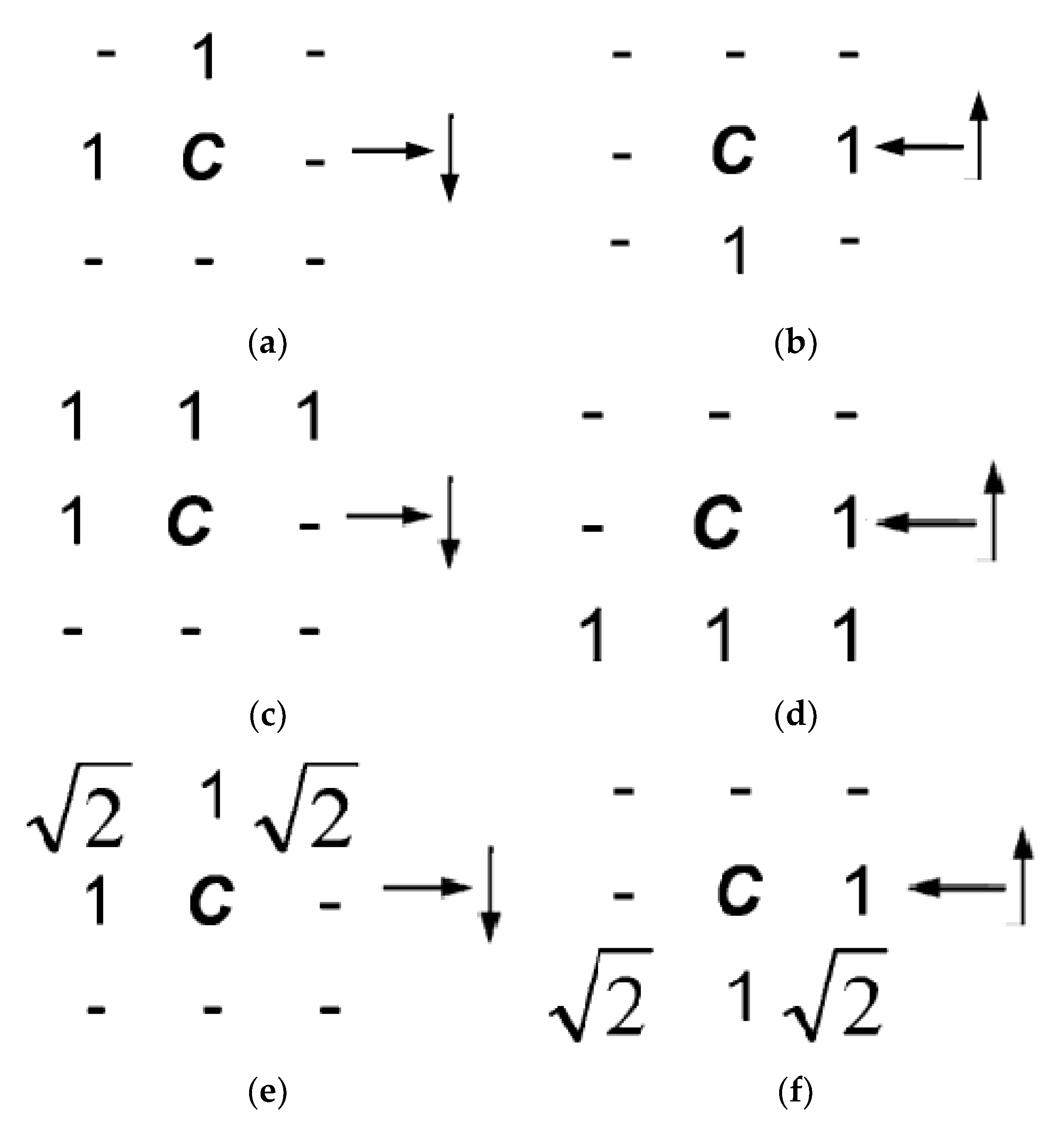
Algorithm 1 shows a sequential raster scan for DT computation based on the Borgefors [10] approach, which consists of initializing the distance map array d to zero for the characteristic pixels and ∞ for the others, and executing a two-phase raster scan for distance propagation with two different scan masks. Each pass employs local neighborhood operations in order to minimize the current distance value assigned to the pixel C = (x,y), located at the center of the mask, by comparing the current distance value with the distance value assigned to each neighbor cell plus the value specified by the mask. Scan masks employed for city block, chessboard, and Euclidean metrics are shown in Figure 1.

Algorithm 1. Sequential Raster Scan DT.
REQUIRE	Img—A binary image
ENSURE	$d$—A bidimentional matrix with distances of Img
	Initialize $d$ for y = each line from the top of the Img then  for x = each cell in the line from left to right then   d(x,y) = min{ d(x,y), d(x,y) + C(x − 1,y), d(x,y) + C(x − 1,y − 1), d(x,y) + C(x,y − 1),       d(x,y) + C(x + 1,y + 1)} for y = each line from the bottom of the Img then  for x = each cell in the line from right to left then   d(x,y) = min{ d(x,y), d(x,y) + C(x − 1,y + 1),      d(x,y) + C(x,y + 1), d(x,y) + C(x + 1,y + 1), d(x,y) + C(x + 1,y)}

Since it is a separable problem, the exact Euclidean distance problem can be treated by reducing the dimension of the input data [2,20,21]. Exploiting this property, the Euclidean distance problem can be solved efficiently using parallelism in columns and rows [30,31,32,37]. However, this process requires that each computation thread has access to a complete column of the image, as well as a common stack structure for the management of potential sites, so its implementation in GPUs and its thread coordination process are relatively complex processes.

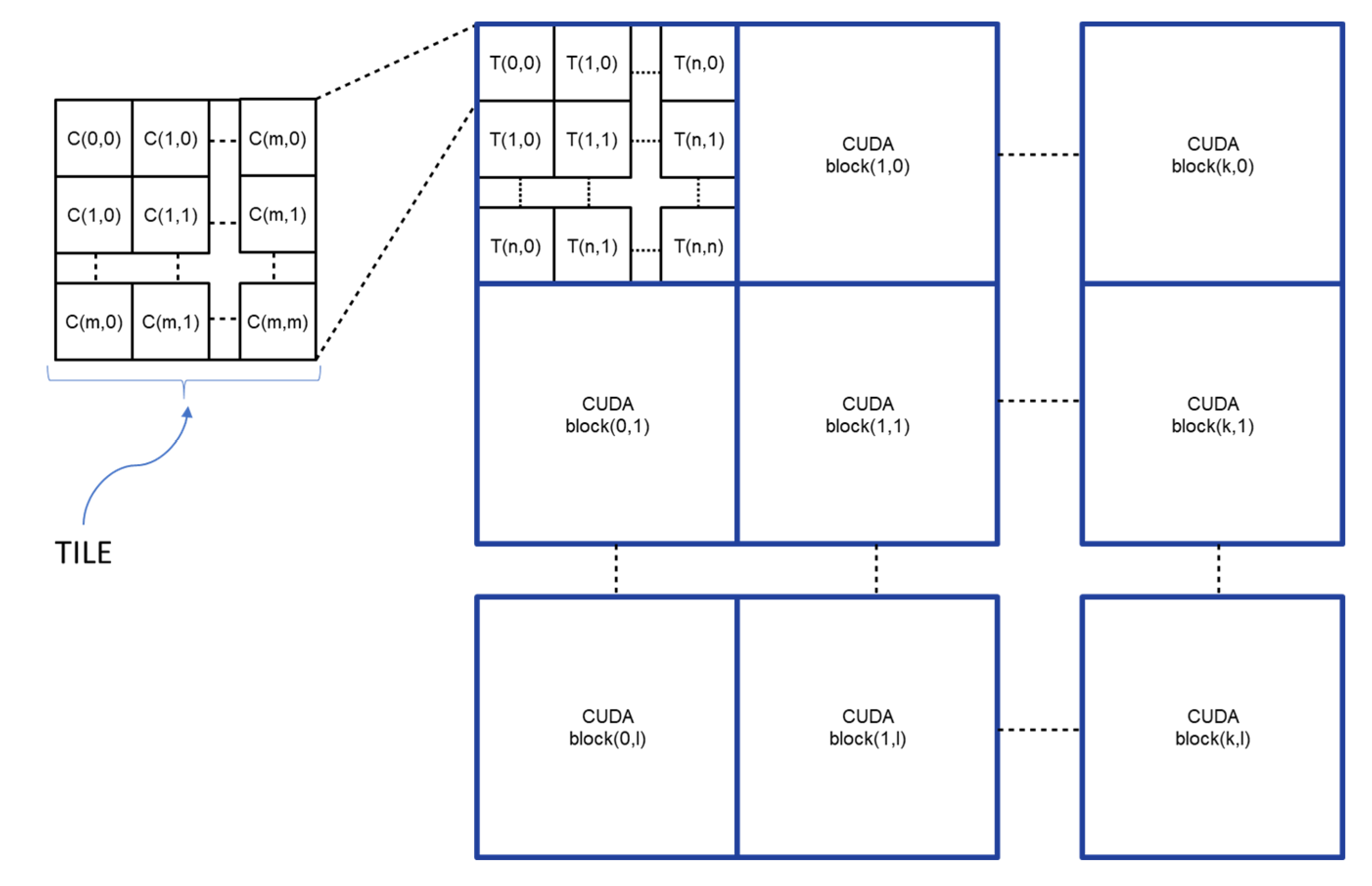
The proposed algorithm, called Parallel Raster Scan for Euclidean Distance Transform (PRSEDT), presents a different approach: the image is set in global memory, and can be accessed via texture memory, and is then processed by a grid of processing blocks. Each block is composed of a set of threads and deals with a quadrangular region of the image (CUDA block); in turn, each region is divided into smaller sections (TILES) in which an individual thread applies a raster algorithm for the propagation of the distance transformation. Each thread works independently until no changes are detected in the entire block, so only a boolean value is required to determine if the block has finished processing. The number of iterations is proportional to the size of the block and the maximum distance in the image, and inversely proportional to the number of regions. The resulting algorithm is highly parallelizable, with few synchronization points and less access to regular memory, making it suitable for implementing in modern GPU architectures, which is reflected in better processing times compared to other state-of-the-art algorithms. Figure 2 shows the representation of what is processed in each thread (a TILE), the CUDA blocks, and the grid of threads blocks.

The algorithm processes an input binary image Img (), of $DIM \times DIM$ pixels, to produce the distance map $DT$ and a Voronoi map $VD$ containing, for each pixel, the coordinates of the closest characteristic point; both arrays are the same size as the input image. Initially, the array $DT$ is initialized to zero for the characteristic pixels and $\infty$ for the others, while the array $VD$ is initialized with the characteristic points pointing to themselves and the other cells without an assigned point, as indicated in Equations (1) and (2).

$$DT\left(x,y\right)=\{\begin{array}{c} \infty , Img\left(x,y\right) = white\\ 0, Img\left(x,y\right) = black\end{array}$$

(1)

$$VD\left(x,y\right)=\{\begin{array}{c}NULL, Img\left(x,y\right) = white\\ \left(x,y\right), Img\left(x,y\right) = black\end{array}$$

(2)

For processing, the image is divided into $k\times l$ blocks, called CUDA blocks. In turn, each block is divided into $n\times n$ tiles that will be processed in parallel by the threads. This scheme guarantees coalesced access to global memory (for writing data) and texture memory (for reading data), improving processing times.

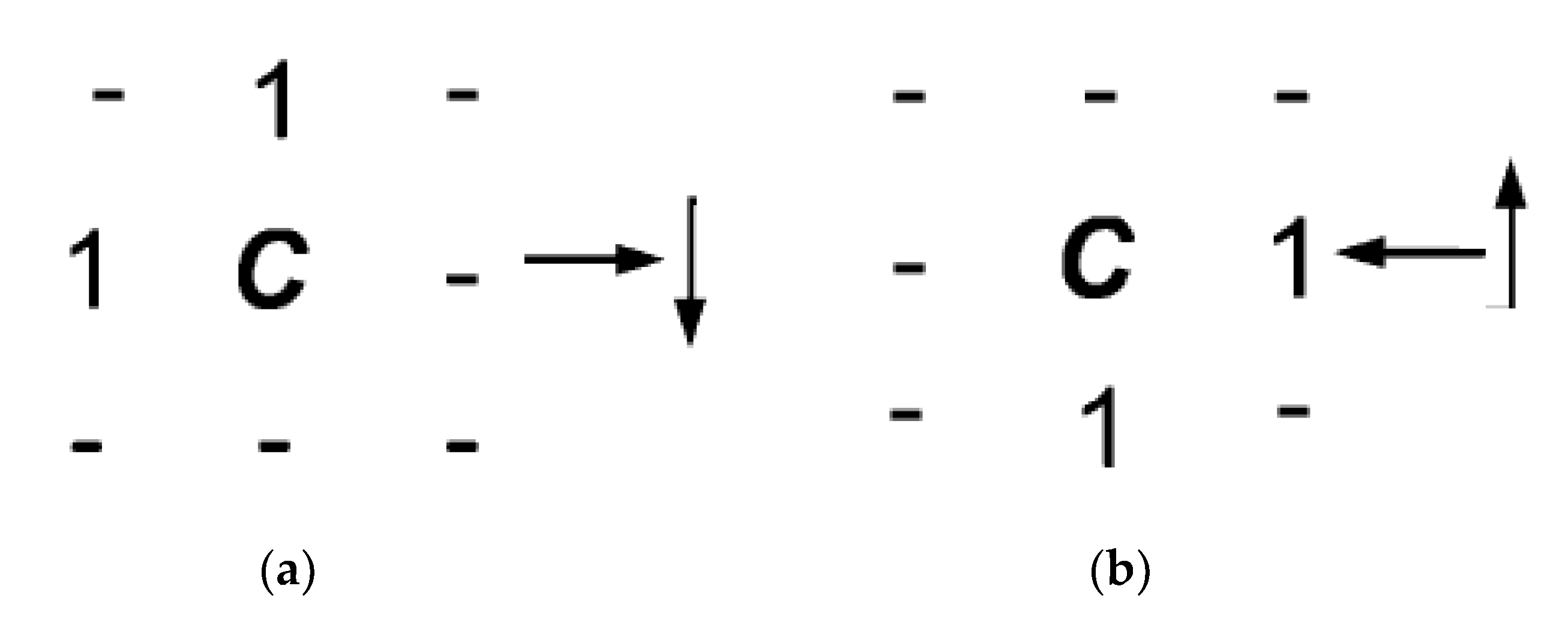
For each tile, a processing thread executes a sequential raster distance propagation algorithm, similar to the chamfer method (Algorithm 1), using mask 1 (Figure 3a) in forwards pass (from left to right, top to bottom) and mask 2 (Figure 3b) in backward pass (from right to left, bottom to top). Both masks only indicate the neighbor pixels that will be considered to update the distance value of the cell $r=\left(x,y\right)$ under consideration. For each of the neighbor pixels indicated by the mask, it is verified whether if the distance from cell $r$ to the pixel pointed by the neighbor is less than the current recorded distance value. If it is true, the matrix $DT$ is updated with the new distance value, and the matrix $VD$ is updated with the identified characteristic point. The above is summarized with Equations (3) and (4).

$$DT\left(r\right)=min\{\begin{array}{c}DT\left(r\right)\\ \Vert r-VD\left(v_i\right)\end{array}$$

(3)

$$VD\left(r\right)=\{\begin{array}{c}\begin{array}{cc}VD\left(v_i\right),& \Vert r-VD\left(v_i\right)\Vert <DT\left(r\right)\end{array}\\ \begin{array}{cc}VD\left(r\right),& \Vert r-VD\left(v_i\right)\Vert \ge DT\left(r\right)\end{array}\end{array}$$

(4)

Rasters on each tile are performed continuously until changes are no longer detected in both $DT$ and $VD$ arrays. The scan masks used in PRSEDT are shows in Figure 3.

Both the size of the tile and the size of the CUDA block are parameters that were determined experimentally, according to the size of the input image and the architecture of the video card, to obtain the best processing time. The maximum size is given by the parameter $m$, which indicates the tile size—i.e., the number of pixels that each thread must process ($m^2$ pixels). The CUDA block size is determined by the parameter $n$, which determines the number of threads processing a CUDA block ($n^2$ threads). In this way, the dimensions of the subimage, which is processed in each CUDA block, are ${\left(n\times m+2\right)}^2$ pixels. The two extra pixels ensure an overlap of one pixel with neighbor blocks to allow the propagation of distance information generated in the block.

To guarantee the proper treatment of the whole input image Img, an array $OB$ of $k\times l$ cells (one cell for each CUDA block) is also used to indicate if each image CUDA block needs to be processed again to update the distance information. The values for the $k$ and $l$ parameters are obtained directly from the dimensions of the input image Img, the size of the CUDA block $n$, and the number of threads per block $m$ (tile resolution).

The proposed method is divided into two algorithms. The Algorithm 2 Main PRSEDT, is in charge of reading the image and copying it to the global memory of the device, invoking the kernel that initializes the $DT$, $VD$ and $OB$ arrays, and determining the number of CUDA blocks and threads per block according to the parameters $n$ and $m$. Next, it invokes the PRSEDTKernel algorithm (Algorithm 3), to propagate the distance information using parallel computing over the CUDA blocks, as many times as necessary, as long as there are changes in the $DT$ and $VD$ arrays.

Algorithm 2. Main PRSEDT
REQUIRE	Img—A binary image
ENSURE	$DT$—A bidimentional matrix with distances of Img
	$VD$—The voronoi diagram of Img
	cudaMemcpy($VD$, Img, cudaMemcpyHostToDevice)//copy Img from Host to Device blocks = (DIM/$n$, DIM/$n$)//Grid dimensions threads = ($n,n$)//Block dimensions initKernel<<blocks, threads>>($DT$, $VD$, $OB)$//Init $DT$ Equation (1), $VD$ Equation (2) and $OB$ blocks = (DIM/($n\times m$),DIM/($n\times m$))//Grid dimensions threads = (n,n)//Block dimensions cudaBindTexture(VD_Tex, VD) ;//Bind the $VD$ in global memory to VD_Tex in texture cudaBindTexture(DT_Tex, DT) ;//Bind the $VD$ in global memory to VD_Tex in texture cudaBindTexture(OB_Tex,OB) ;//Bind the $VD$ in global memory to VD_Tex in texture $count\leftarrow 1$ $ctrl\leftarrow 1$ repeat  $flag\leftarrow false$//use memSet to set false the flag of the device  blocks(DIM/($n\times m$),DIM/($n\times m$))//Grid dimensions  threads($n,n$)//Block dimensions  PRSEDTKernel <<blocks,threads>>($DT$, $VD$, $OB$, $flag$, $ctrl$)  $count\leftarrow count+1$  if $count>2$ then   $ctrl\leftarrow {\left(\left(count-2\right)\times n\times m/2\right)}^2$  else   $ctrl\leftarrow coun{t}^2$  Use cudaMemcpy to copy back the flag from device to host until $!flag$ float *DT_Host = (float*)malloc(imageSize); cudaMemcpy(DT_Host, $DT$, cudaMemcpyDeviceToHost); int *VD_Host = (int*)malloc(imageSize); cudaMemcpy(VD_Host, $VD$, cudaMemcpyDeviceToHost);

Algorithm 3.
PRSEDTKernel (*$DT$, *$VD$, *$OB$, *$flag$, *$ctrl)$
	__shared__ bool $\mathrm{shOpt}$ __shared__ int $\mathrm{optimized}$ int $\mathrm{optreg}\leftarrow 0$ if $threadIdx.x==0$ AND $threadIdx.y==0$ then  $optimized\leftarrow 0$  $\mathrm{shOpt}\leftarrow \mathrm{false}$  if $\mathrm{OB}\_Tex\left[blockIdx.x+blockIdx.y*gridDim.x\right]==1$ then   $shOpt\leftarrow true$ syncthreads(); if $shOpt$ then  return shared float $memC\left[n\times m\right]\left[n\times m\right]$ shared int $ptr\left[n\times m+2\right]\left[n\times m+2\right]$ shared bool $shEnter$; $memC\leftarrow DT\_Tex\mathrm{TILE}\mathrm{of}{m}^2$ (access in a coalesced form) for each cell in $TILEofmemC$  if ${\mathrm{memC}}_{\mathrm{cell}}\le \mathrm{ctrl}$ then   $\mathrm{optreg}++$ atomicAdd($optimized,optreg$) syncthreads() if $\mathrm{optimized}=={\left(n\times m\right)}^2$ then  $\mathrm{OB}\left[\mathrm{blockIdx}.\mathrm{x}+\mathrm{blockIdx}.\mathrm{y}\times \mathrm{gridDim}.\mathrm{x}\right]\leftarrow \mathrm{true}$  return $\mathrm{ptr}\leftarrow VD\_Tex\mathrm{TILE}\mathrm{of}{\left(n\times m+2\right)}^2$ (access in a coalesced form) repeat  syncthreads();  if $\mathrm{threadIdx}.\mathrm{y}==0$and $\mathrm{threadIdx}.\mathrm{x}==0$ then    $\mathrm{shEnter}\leftarrow \mathrm{false}$   syncthreads();  for each line from the top of the TILE then   for each cell in the line of the TILE from left to right then    apply scan mask 1 (Figure 3a)    evaluate $\mathrm{memC}$ and $\mathrm{ptr}$ according to Equations (3) and (4).    if any update is made then     $shEnter\leftarrow \mathrm{true}$  for each line from the bottom of the TILE then   for each cell in the line of the TILE from right to left then    apply scan mask 2 (Figure 3b)    evaluate $\mathrm{memC}$ and $\mathrm{ptr}$ according to Equations (3) and (4).    if any update is made then     $shEnter\leftarrow \mathrm{true}$  syncthreads() until $!shEnter$ if any change in the TILE then  update $DT$ with corresponding TILE of $\mathrm{memC}$  update $VD$ with corresponding TILE of $\mathrm{ptr}$  $\mathrm{flag}\leftarrow \mathrm{true}$

The PRSEDTKernel algorithm, shown in Algorithm 3, handles the parallel processing of the CUDA blocks. Initially, the first thread of each block checks if the assigned block requires updating, using the array $OB$. If the block requires no processing, the entire block ends. If processing is required, an array $memC$ is created in the shared memory space, and each thread of the block makes a copy of the distance map $DT$ of its respective tile, through a coalesced access to texture memory. Next, the threads of the block verify if, for each cell within its respective tile, the distance value is less than a threshold value $ctrl$ (which increases according to the number of iterations, in Algorithm 2 Main PRSEDT). If this condition is verified for all the pixels of the block, then the block is considered as optimized and does not require to be processed again, so the corresponding cell in the array $OB$ is updated and the complete block ends.

If the distance map of this block can still be improved, then each thread makes a copy of its respective tile of the Voronoi diagram $VD$, from the texture memory to the shared array $ptr$, with coalesced memory access. From this moment, each thread propagates the distance information in its respective tile, using the sequential raster process described above, until all the threads no longer generate changes.

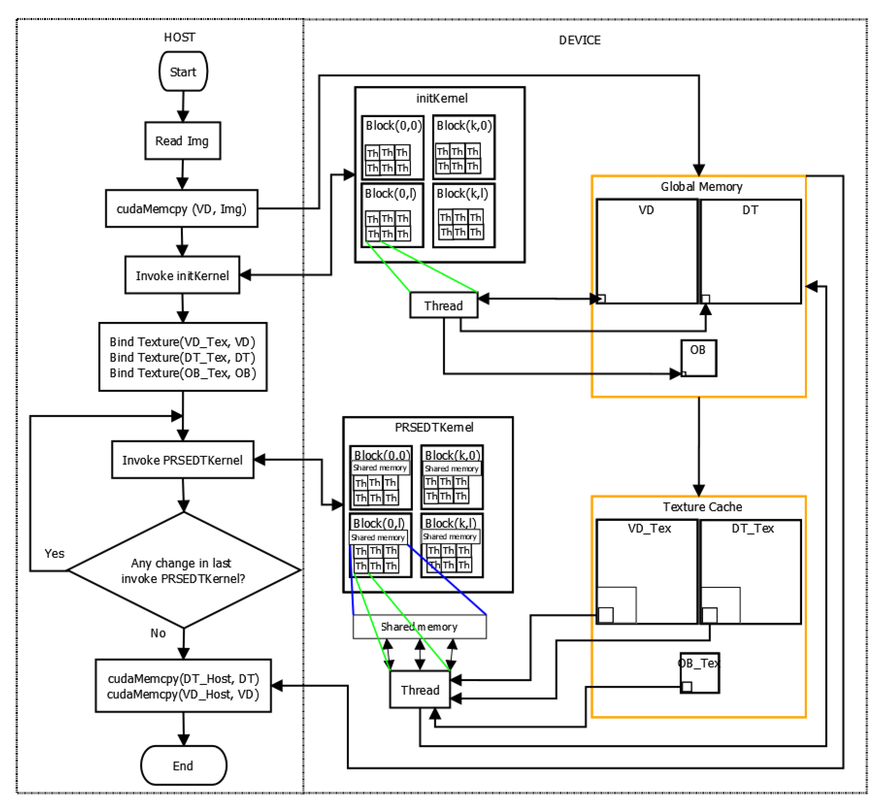
Finally, if any changes were made to the block, then the $DT$ and $VD$ arrays in global memory are updated, with the data stored in the arrays $memC$ and $ptr$ in the block’s shared memory. Figure 4 shows a flowchart of the heterogeneous programming model used in PRSEDT: on the left side we can see the process running in host, and on the right side the processes running in device, in order to show the whole coordination of our approach. Briefly, the host is in charge of reading the image and copying it to the global memory of the device, instantiating the kernels and copying back the Voronoi diagram and the distance transform; the device, on the other hand, is in charge of initializing the Voronoi diagram, the distance transform map, and the array OB (initKernel); finally, each thread of PRSEDTKernel processes a tile of VD and DT.

3. Results

For experimentation purposes, the implementation of the proposed algorithm was carried out in a desktop computer equipped with an Intel Core i7-7700 processor, with eight cores at 3.6 GHz, and an NVIDIA GeForce GTX 1070 video card. The operating system used is Ubuntu 18.04 LTS 64-bit, and the programming language is C++ with CUDA 10.2. We used a NVIDIA “Visual Profiler” to obtain information about the data transfer between the device memory and the host memory, as well as the computation performed by the GPU card.

To evaluate the proposed method, the decision was made to compare it with the PBA+ [37] algorithm, an updated revision of the PBA algorithm [29]. The original PBA algorithm proved to be highly competitive compared to the two most representative state-of-the-art algorithms: Schneider et al.’s [33] and JFA [32]. In its PBA+ version, the authors have achieved significant improvements to the implementation of their original algorithm, with better processing times. In addition, on their website, the authors generously share the source code of their implementation, as well as the recommended values of the different parameters of their algorithm, according to the characteristics of the input image and the video card used. Due to these two factors, we consider that the PBA+ algorithm is a representative state-of-the-art algorithm in the calculation of the distance map in parallel hardware architectures.

It is important to highlight that the distance maps obtained by the PBA+ algorithm and our proposed algorithm (PRSEDT) are exactly the same for all the input images used in experimentation, so the difference between both algorithms is in the performance at runtime and not in the precision of the obtained distance map.

Table 1. Parameters for the improved Parallel Banding Algorithm (PBA+).

Texture Size	m1	m2	m3
512 × 512	8	16	8
1024 × 1024	16	32	8
2048 × 2048	32	32	8
4096 × 4096	64	32	4
8192 × 8192	64	32	4
16,384 × 16,384	128	32	4

shows the parameters proposed by the authors of the PBA+ algorithm for different image resolutions and the GPU card used in this experimentation, where m1, m2 and m3 are the parameters of each phase in the PBA+ algorithm. On the other hand,

Table 2. Parameters for PRSEDT. $m$ is tile resolution and $n$ is the block size.

Texture Size	TILERES	BSIZE
512 × 512	2	8
1024 × 1024	2	8
2048 × 2048	2	8
4096 × 4096	4	8
8192 × 8192	4	8
16,384 × 16,384	4	8

shows the parameters used for our proposed method (PRSEDT), for different image resolutions, obtained by own experimentation.

In order to evaluate the impact of memory transfers from host to device and vice versa, we carried out a set of experiments from which we obtained the transfer time. From

Table 3. Memory transfer times (milliseconds). Column HostToDevice indicates the transfer time of the image from the host to the device, while the DeviceToHost columns indicate the transfer time from the device to the host of the Distance transform (DT) and Voronoi diagram (VD) matrices, respectively.

Texture Size	PRSEDT			PBA+
	HostToDevice	DeviceToHost		HostToDevice	DeviceToHost
512 × 512	0.082	0.08042	0.0881	0.082	0.0809	0.0811
1024 × 1024	0.598	1.31	1.28	0.593	1.28	1.27
2048 × 2048	2.7979	6.49	6.56	2.91	6.35	6.19
4096 × 4096	12.11	26.95	26.93	12.1	26.79	26.68
8192 × 8192	49.5	108.64	108.89	48.8	108.72	109.01
16,384 × 16,384	191.63	438.94	439.01	194.01	438.61	438.5

it can be noted that the transfer time is affected only by the dimensions of the image and is similar for both PRSEDT and PBA+ algorithms. Therefore, in the next experiments, we focus on evaluating the processing time of the algorithms.

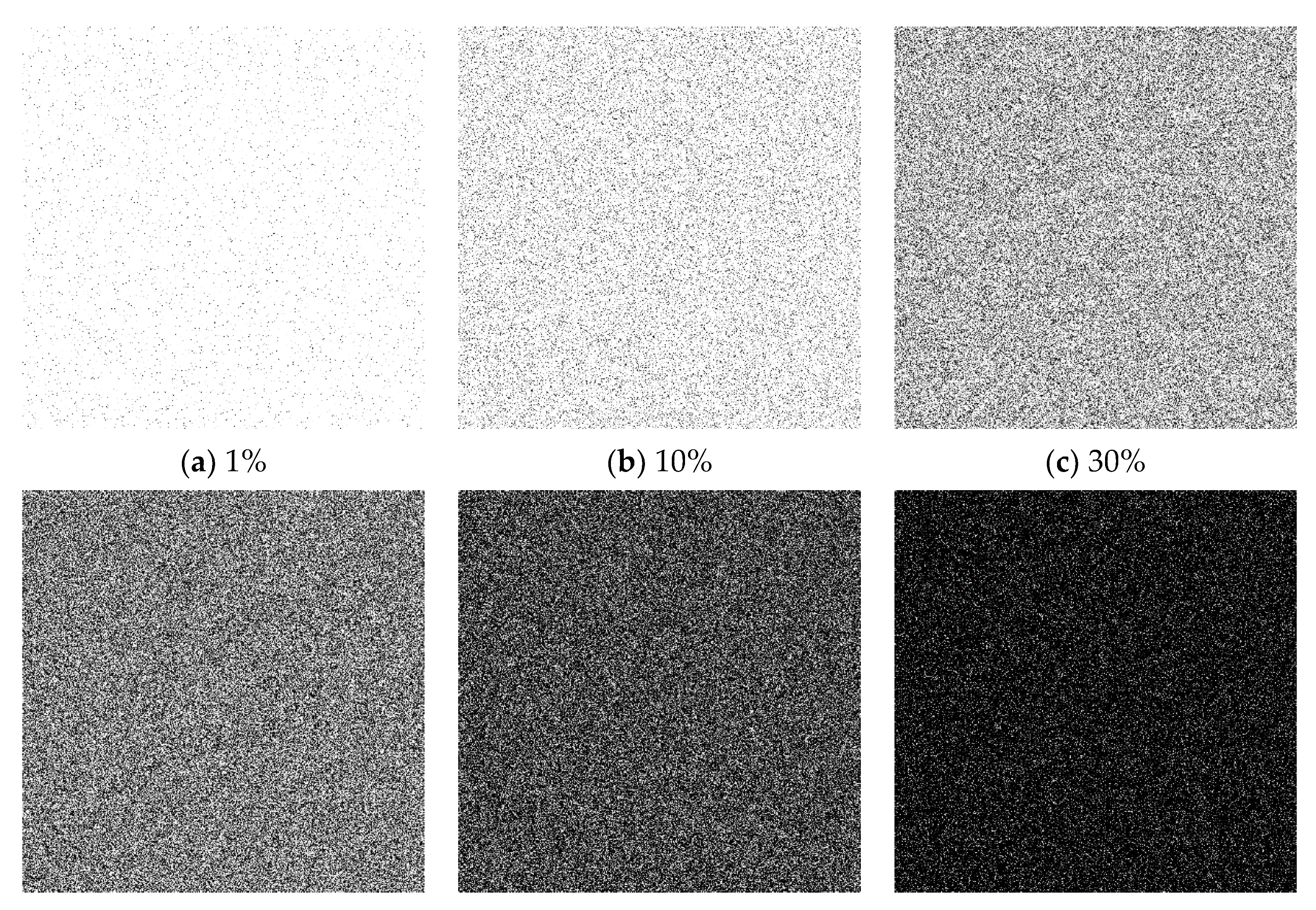
In the first phase of experimentation, the performance of the algorithms for input images of different resolutions and with different densities of randomly generated feature points was compared. The density of random feature points took values of 1%, 10%, 30%, 50%, 70% and 90%, with resolutions of $512 \times 512$, $1024\times 1024$, $2048\times 2048$, $4096\times 4096$, $8192\times 8192$ and $16384\times 16384$. Figure 5 shows an example of the set of images of $1024\times 1024$ pixels of resolution, for different density values.

Table 4. Running time (milliseconds) of each image with different densities of black pixels and different resolutions.

Density	Algorithm	$512\times 512$		$1024\times 1024$		$2048\times 2048$
		ms	Speedup	ms	Speedup	ms	Speedup
1%	PBA+	0.335	1.044	0.801	0.803	2.545	0.745
	PRSEDT	0.321		0.998		3.415
10%	PBA+	0.38	1.827	0.968	1.763	3.111	1.590
	PRSEDT	0.208		0.549		1.956
30%	PBA+	0.41	2.343	1.066	2.406	3.214	2.169
	PRSEDT	0.175		0.443		1.482
50%	PBA+	0.408	2.684	1.074	3.294	3.181	3.233
	PRSEDT	0.152		0.326		0.984
70%	PBA+	0.395	3.110	1.034	3.517	2.996	3.428
	PRSEDT	0.127		0.294		0.874
90%	PBA+	0.382	3.441	0.985	3.717	2.87	3.470
	PRSEDT	0.111		0.265		0.827
Density	Algorithm	$4096\times 4096$		$8192\times 8192$		$16,384\times 16,384$
		ms	Speedup	ms	Speedup	ms	Speedup
1%	PBA+	8.89	0.800	30.49	0.881	117.87	0.865
	PRSEDT	11.11		34.61		136.24
10%	PBA+	10.25	1.253	36.13	1.401	136.95	1.363
	PRSEDT	8.18		25.79		100.5
30%	PBA+	10.21	1.383	36.94	1.564	139.28	1.481
	PRSEDT	7.38		23.62		94.04
50%	PBA+	9.93	2.315	35.82	2.588	135.99	2.508
	PRSEDT	4.29		13.84		54.23
70%	PBA+	9.44	2.275	34.06	2.604	130.15	2.503
	PRSEDT	4.15		13.08		52
90%	PBA+	9.01	2.346	32.78	2.646	121.08	2.478
	PRSEDT	3.84		12.39		48.86

shows the processing time in milliseconds and the speedup factor obtained for images of different densities and resolutions. In $512\times 512$ resolution images, the PRSEDT improves the performance of the PBA+ algorithm in all cases, with speedup factors ranging from $1.044$ for $1\%$ density images to $3.441$ for images with $90\%$ density.

For $1024\times 1024$ pixel resolution images, the PBA+ algorithm performs better on $1\%$ density images, but our PRSEDT algorithm achieves better results for images with $10\%$ to $90\%$ density, with speedup factors ranging from $1.763$ to $3.717$.

In the case of $2048\times 2048$ resolution images with $1\%$ density, the speedup factor was $0.745$, so the PBA+ algorithm obtains better results than PRSEDT; however, for densities from $10\%$ to $90\%$, our algorithm performs better, with speedup factors ranging from $1.590$ to $3.470$.

For images with a resolution of $4096\times 4096$ pixels, the performance pattern is repeated: for 1% density there is a speedup factor of $0.800$, and the PBA+ algorithm obtains better results than our method. Nevertheless, for densities from $10\%$ up to $90\%$, the proposed method performs better, with speedup factors ranging from $1.253$ to $2.346$.

With $8192\times 8192$ resolution images, we obtained a speedup factor of $0.881$ for a density of $1\%$, and for densities from $10\%$ to $90\%$, the speedup factor ranges from $1.401$ to $2.646$.

Finally, for images with a resolution of $16,384\times 16,384$, the obtained speedup factor for $1\%$ density is $0.865$, while for densities of $10\%$, $30\%$, $50\%$, $70\%$ and $90\%$, the speedup factors are $1.363$, $1.481$, $2.508$, $2.503$ and $2.478$, respectively.

From the data of Table 3, we can see that in 31 out of the 36 cases PRSEDT yields better results than the PBA+. The better performance of PBA+ in low-density images can be explained because, as mentioned above, the number of iterations of the proposed method is proportional to the maximum image distance, which is greater in very low-density images. However, it can be observed that in most cases (21 out of 36) a speedup factor greater than 100% is obtained, even tripling the performance of the PBA+ algorithm in some cases.

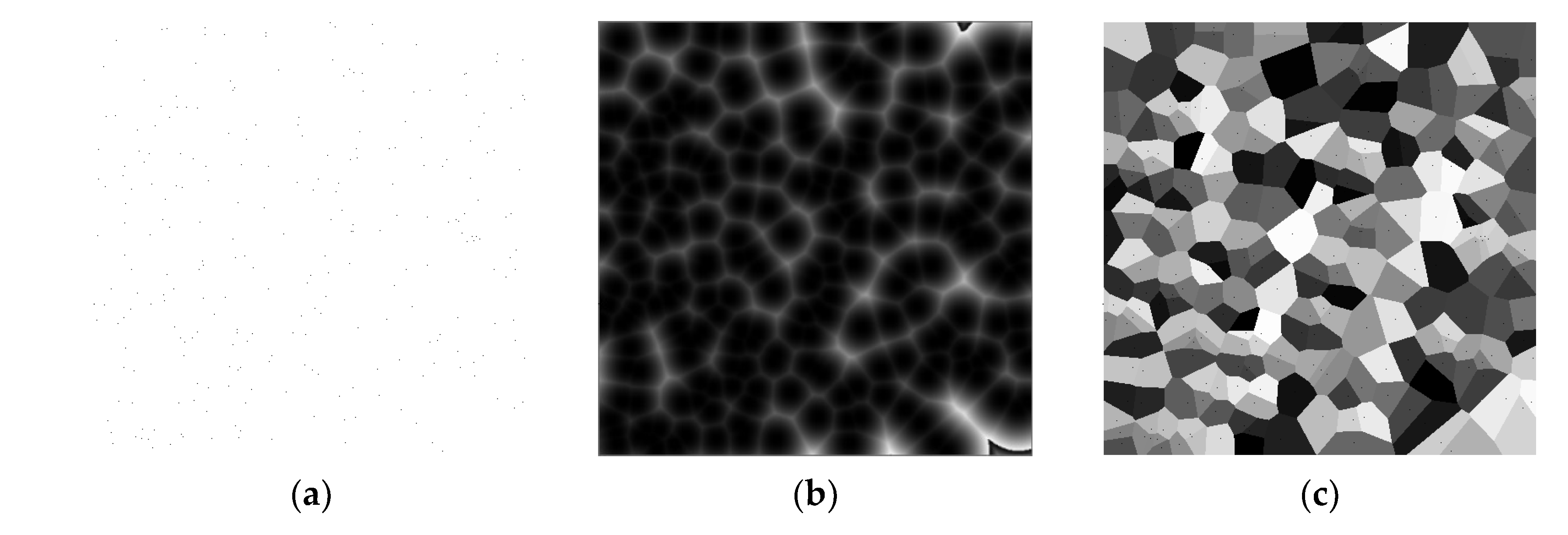
Figure 6 shows an example of the results obtained for an input image with random feature points (Figure 6a) with the grayscale distance map (Figure 6b) and the Voronoi diagram (Figure 6c).

Table 5. PRSEDTKernel instances.

Density	$512\times 512$	$1024\times 1024$	$2048\times 2048$	$4096\times 4096$	$8192\times 8192$	$16,384\times 16,384$
1%	4	4	5	4	4	4
10%	3	3	3	3	3	3
30%	3	3	3	3	3	3
50%	3	3	3	3	3	3
70%	2	2	2	3	3	3
90%	2	2	2	3	3	3

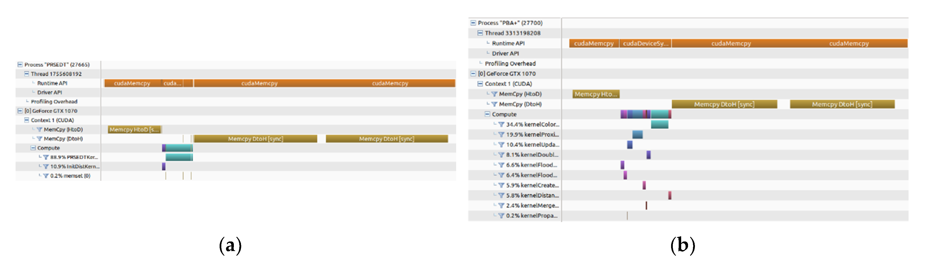
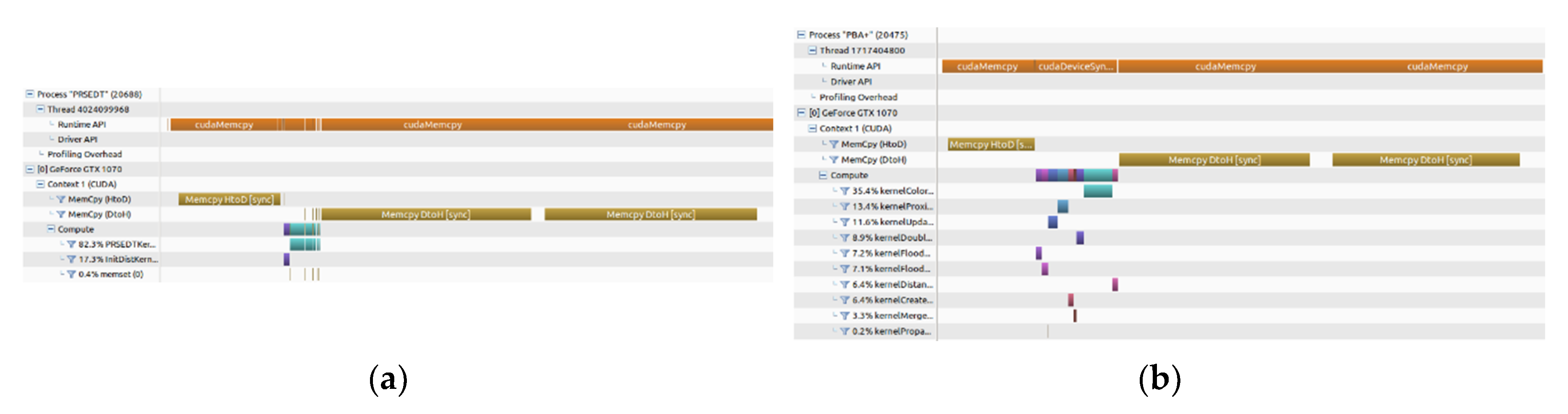
shows, for each resolution and for each density of black pixels, the number of times the PRSEDTKernel was instantiated. As can be seen, the higher the density the fewer instances needed, which is related to the maximum value in the distance map. Figure 7 shows the timeline of the execution of the PRSEDT algorithm and the PBA+ algorithm for an input image of 2048 × 2048 pixels and a density of 30%. On the one hand, our PRSEDT algorithm instance only has two kernels: the initKernel for initialization of DT and VD matrices, and the PRSEDTKernel three times (Figure 7a) for distance propagation. On the other hand, the PBA+ algorithm requires instantiating 10 different kernels, making its implementation more complex (Figure 7b).

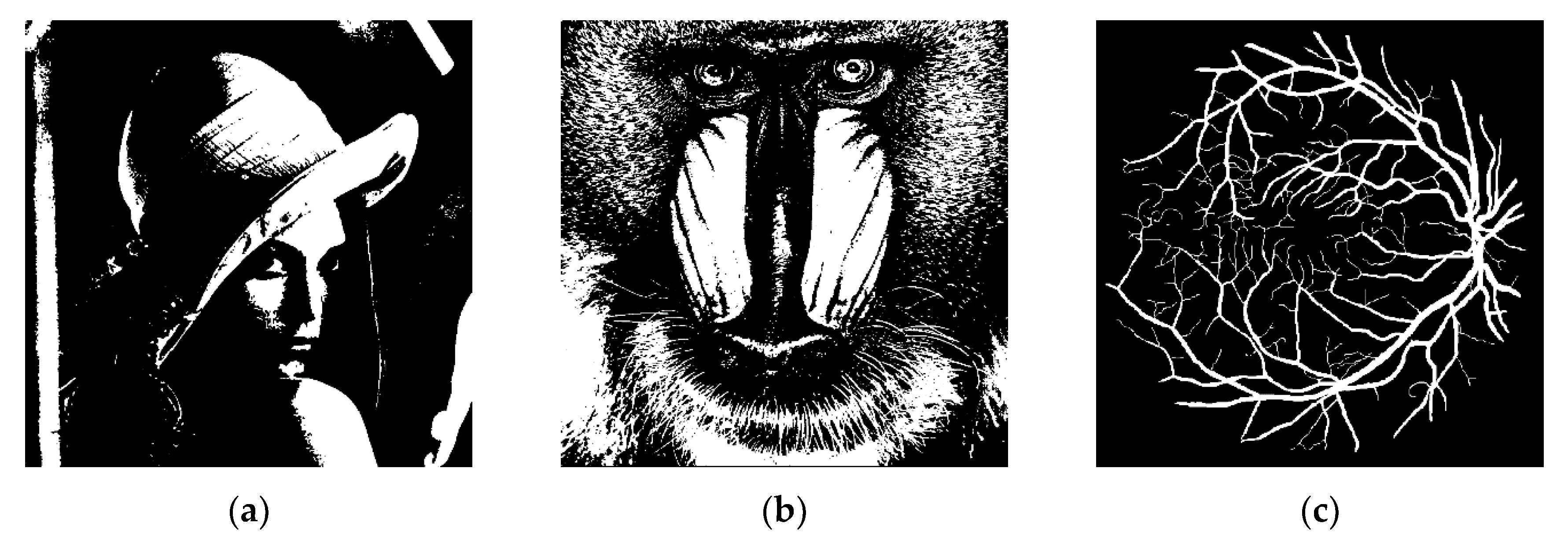
In the second phase of experimentation, the performance of the proposed algorithm for specific binary images was verified. The Lena, Mandril and Retina images were taken as input images (Figure 8), with resolutions of $512\times 512$, $1024\times 1024$, $2048\times 2048$, $4096\times 4096$, $8192\times 8192$ and $16,384\times 16,384$ pixels. The results are summarized in

Table 6. Running time (milliseconds) of each image with different input images and different resolutions.

Image	Algorithm	512 × 512		1024 × 1024		2048 × 2048
		ms	Speedup	ms	Speedup	ms	Speedup
Lena	PBA+	0.401	1.604	1.029	1.790	2.87	1.535
	PRSEDT	0.25		0.575		1.87
Mandril	PBA+	0.434	1.507	1.074	1.554	2.99	1.187
	PRSEDT	0.288		0.691		2.52
Retina	PBA+	0.402	2.871	0.993	3.193	2.82	3.099
	PRSEDT	0.14		0.311		0.91
Image	Algorithm	4096 × 4096		8192 × 8192		16,384 × 16,384
		ms	Speedup	ms	Speedup	ms	Speedup
Lena	PBA+	8.68	1.072	29.69	1.107	116.93	0.809
	PRSEDT	8.1		26.82		144.51
Mandril	PBA+	9.24	0.857	30.81	0.812	116.66	0.566
	PRSEDT	10.78		37.94		206.29
Retina	PBA+	8.72	2.047	30.24	2.625	114.24	2.587
	PRSEDT	4.26		11.52		44.16

, with the execution time in milliseconds and the speedup factor with respect to the PBA+ algorithm for each of the images.

Table 7. Number of PRSEDTKernel instances required to process the input image.

Image	$512\times 512$	$1024\times 1024$	$2048\times 2048$	$4096\times 4096$	$8192\times 8192$	$16,384\times 16,384$
Lena	5	8	14	15	27	51
Mandril	6	8	14	14	28	54
Retina	3	4	5	5	7	11

shows, for each resolution and input image from Figure 8, the number of times that the PRSEDTKernel was instantiated. Since the Mandril and Lena input images have wider white areas, the maximum distance value is greater than in the Retina image. This fact is reflected in the greater number of instantiations required of the PRSEDTKernel to propagate the distance information among tiles and CUDA blocks in these large white areas, thus delaying the propagation of the distance transformation. The Retina image requires fewer instances due to smaller areas of white pixels.

For the Lena image (Figure 8a), it can be seen that the proposed algorithm improves the performances of the PBA+ algorithm by a factor of $1.604$ for the $512\times 512$ resolution, $1.790$ for the $1024\times 1024$ resolution, $1.535$ for the $2048\times 2048$ resolution, $1.072$ for the $4096\times 4096$ resolution and finally $1.107$ for $8192\times 8192$ resolution. In the case of the $16,384\times 16,384$ resolution, the PBA+ algorithm showed a better performance, with a speedup factor of $0.809$. 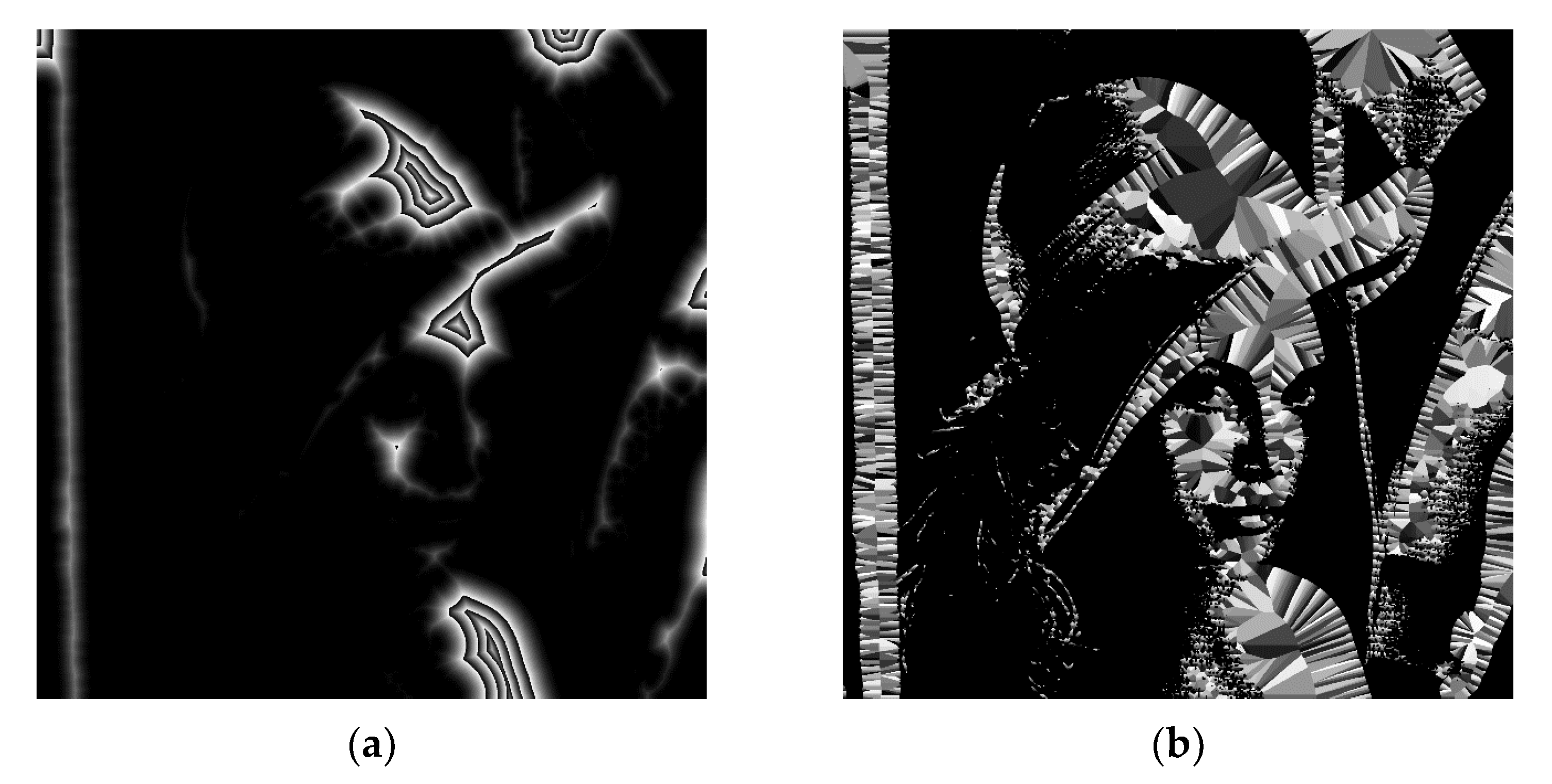Figure 9 shows the resulting distance map and Voronoi diagram for the $2048\times 2048$-pixel Lena image.

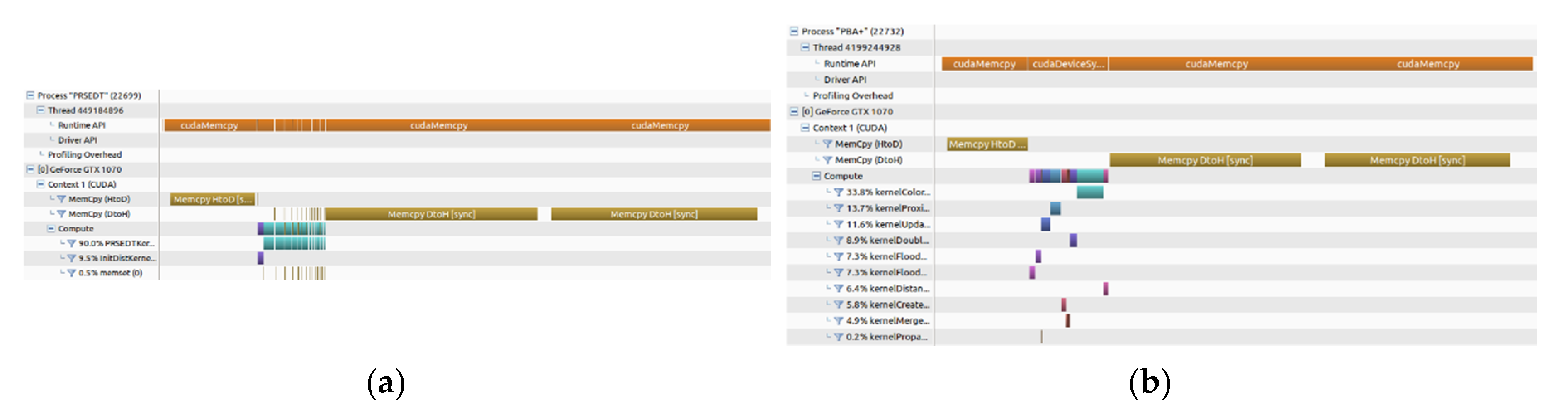
Figure 10 shows the timelines for the PRSEDT algorithm and the PBA+ algorithm, while processing the Lena input image of 2048 × 2048 pixels. The PRSEDT algorithm (Figure 10a) is required to instantiate the PRSEDTkernel 14 times (as reported in Table 6), each instantiation requiring a reset of the global flag at the beginning and a memcopy from the device to host to verify the result of the flag at the end of the PRSEDTKernel execution. The times required for these data transfers are considered in the total processing time. On the other hand, the PBA+ algorithm does not require additional memory data transfers between host and device; however, the total processing time is higher than our approach (Table 6).

For the Mandril image (Figure 8b), it can be seen that our proposal improves the performance of the PBA+ algorithm in resolutions of $512\times 512$, $1024\times 1024$, and $2048\times 2048$ pixels, with speedup factors of $1.507$, $1.554$, and $1.187$, respectively. The PBA+ algorithm showed better results for the resolutions of $4096\times 4096$, $8192\times 8192$, and $16,384\times 16,384$ pixels, with speedup factors of $0.857$, $0.812$ and $0.566$, respectively. 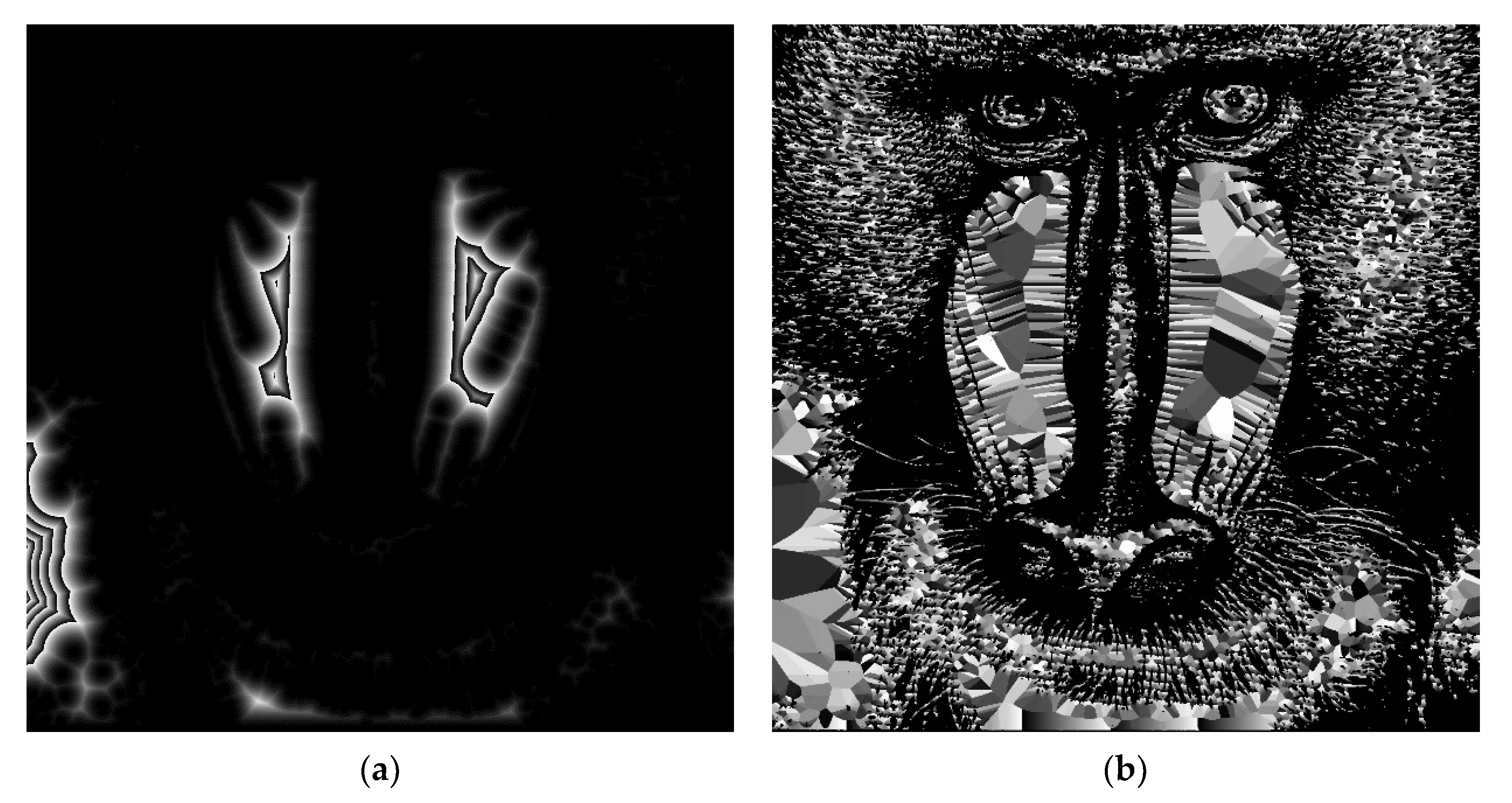The results obtained for the $2048\times 2048$-pixel image are shown in Figure 11.

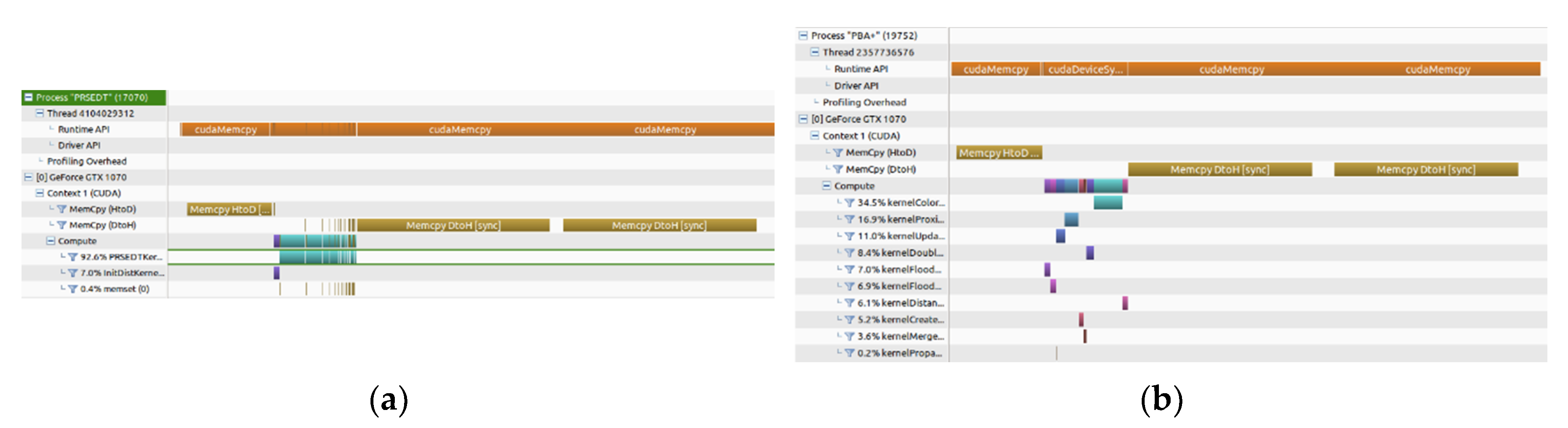
Figure 12 shows the timeline of the execution of the PRSEDT algorithm and the PBA+ algorithm for the 2048 × 2048 pixels Mandril input image. As for the Lena image, we can see in Figure 12a that PRSEDT algorithm requires to instantiate 14 times the PRSEDTkernel (Table 6) to process the whole image, with their respective memory data transfers of the flag value between the Host and the Device. However, the total processing time is lower than the PBA+ algorithm (Figure 12b).

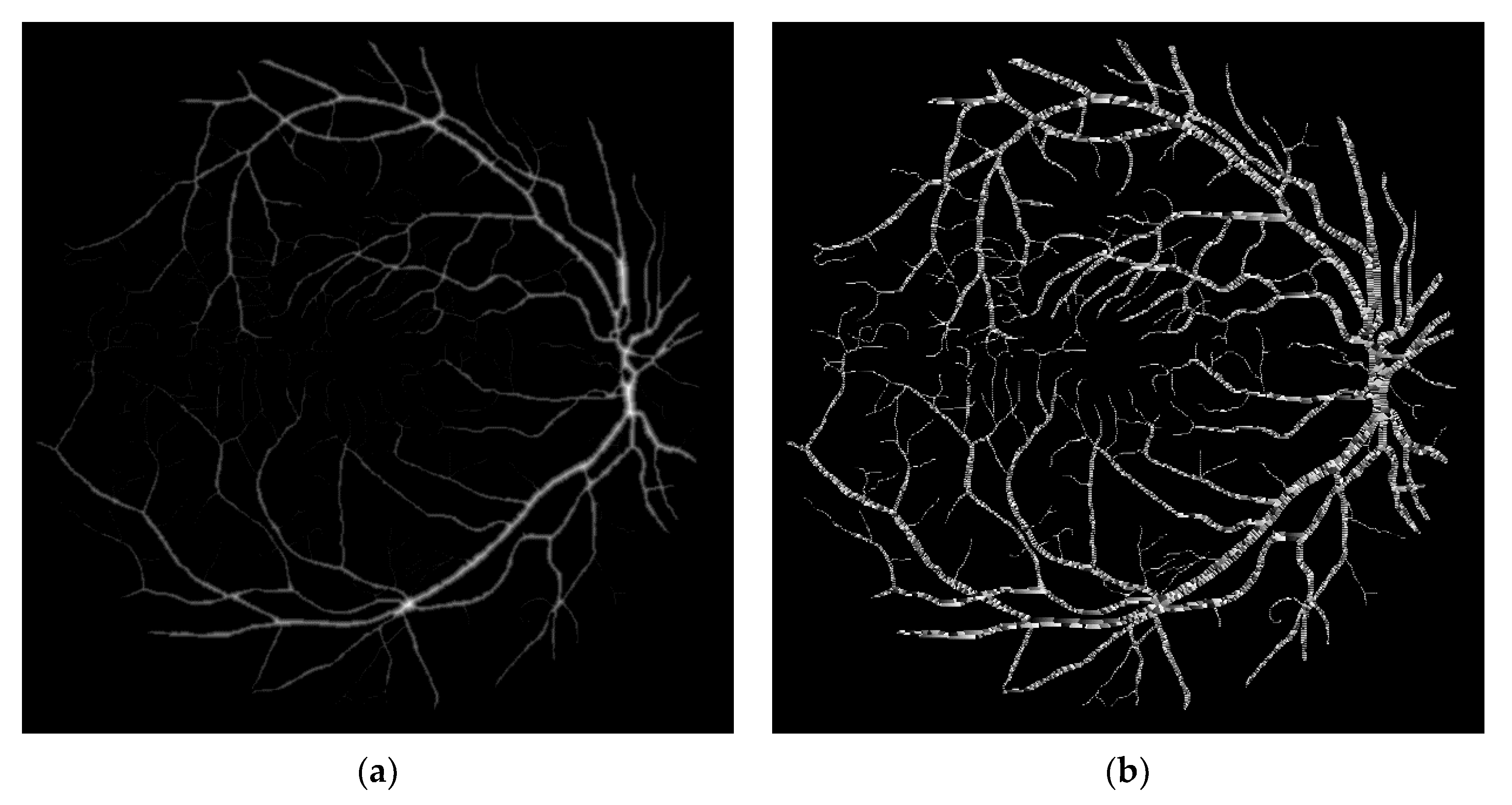
Finally, for the Retina image (Figure 8c), the proposed method improves the performance of the PBA+ algorithm in all cases, with speedup factors of $2.871$ for the resolution of $512\times 512$, of $3.193$ in the image of $1024\times 1024$ pixels, of $3.099$ for the resolution of $2048\times 2048$, of $2.047$ for the resolution of $4096\times 4096$, of $2.625$ for the $8192\times 8192$-pixel image, and for a resolution of $16,384\times 16,384$ pixels the execution time was improved by $2.587$. The results obtained for the Retina image and $2048\times 2048$-pixel image are shows in Figure 13.

Figure 14 shows the profiles of the PRSEDT algorithm and the PBA+ algorithm while processing the 2048 × 2048-pixel Retina input image. Since this image has smaller white areas, the PRSEDT algorithm only requires five instances of the PRSEDTkernel to process the image. This image shows the true potential of our algorithm: a simpler algorithm can outperform a more complex algorithm.

4. Conclusions

In this document, a new parallel algorithm is proposed for the computation of the exact Euclidean distance map of a binary image. In this algorithm, a new approach is proposed that mixes CUDA multi-thread parallel image processing with a raster propagation of distance information over small fragments of the image. The way in which these image fragments are organized, as well as the coalesced access to global and texture memory, allow better use of the architecture of modern video cards, which is reflected in the better processing times, both in small and large images.

The PBA algorithm, in 2010, turned out to be a much more competitive algorithm than the other state-of-the-art approaches at the time. Even now, the PBA algorithm is a reference in the literature of the research area. On their website, the authors of the PBA+ algorithm show that this variant is faster than the original algorithm, significantly improving its performance in all cases, particularly in large-size images with a significant density of feature points.

Therefore, together with the possibility of directly obtaining the source code of this algorithm, we decided to use the PBA+ algorithm as a reference control to evaluate the proposed approach’s performance.

From the experimentation carried out, we can verify that, in most cases, the proposed algorithm performs better than the PBA+ algorithm, obtaining speedup factors that even reach 3.193—that is, they divide the required processing time by three. There are some situations where the PBA+ algorithm is better, particularly in images where the largest distance value is relatively large, which occurs in high-resolution images with a low density of feature points. Even in these cases, the performance loss of our algorithm is around 20% only in most cases.