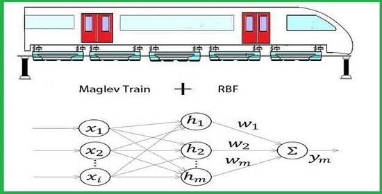
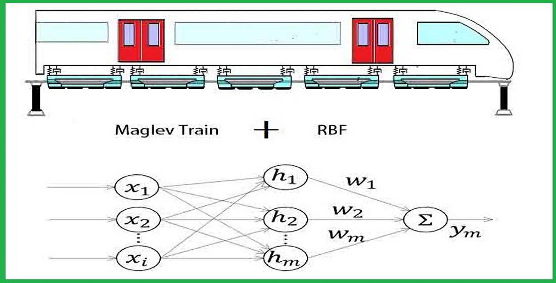
Research of RBF-PID Control in Maglev System

Abstract

Control of the maglev system is one of the most significant technologies of the maglev train. The common proportion integration differentiation (PID) method, which has fixed control parameters, ignores the non-linearity and uncertainty of the model in the design process. In the actual process, due to environmental changes and interference, the inherent parameters of the system will drift significantly. The traditional PID controller has difficulty meeting the control requirements, and will have poor control effect in the actual working environment. Therefore, a radial basis function (RBF)-PID controller is designed in this article, which can use the information from the levitation system identified by the RBF network to adjust the parameters of the controller in real time. Compared with the traditional PID control method, it is shown that the RBF-PID method can improve the control performance of the system through simulation and experiment.

1. Introduction

As a new type of transportation with many advantages such as little noise and vibration, less abrasion and environmental dependence, the maglev train will play a crucial role in future traffic systems. It meets the needs of comfort, safety, convenience and high efficiency [1]. The controller of the maglev train is arranged symmetrically on the left and right sides of the train. Normally, we focus on the controller on one side of the maglev train, and the other side is the same to a certain extent. With the symmetrical structure in the control system of the maglev train, research on control technology in the maglev train can be simpler. The control algorithm for maglev is one of the most important technologies, which often needs to establish an accurate model of the maglev system. Maria Hypiusova designed the proportion integration differentiation (PID) controller for the magnetic levitation model with a method accomplished with performance specification in terms of phase margin and the modification of the Neimark D-partition method, which ensures the desired phase margin [2]. Ishtiaq Ahmad presented the design of the PID controller for a magnetic levitation system based on an efficient method of tuning controller parameters using the genetic algorithm [3]. Since the maglev system is a highly non-linear system, traditional PID control with fixed controller parameters will have poor control performance when the system is interfered with by the external environment changing or with some internal parameters drifting. In the maglev levitation module, the air gap between the track and the electromagnet is generally kept unchanged at about 8 mm [4,5], and the deterioration of the control performance may cause more severe consequences, so a better method is needed.

At present, the research into artificial intelligence, machine learning and big data is in a stage of rapid development. The intelligent control currently appearing in the field of control provides new methods and new theories in the research on robots, drones, etc. [6]. Artificial intelligence and other new theories can solve some difficult problems in the traditional control field [7]. The neural network built by imitating the neuron structure in the brain can approximate non-linear functions to some extent, and it is very helpful for the identification and control of the non-linear system. Compared with the previous traditional control method, it improves the control performance, and has a certain robustness to some disturbances and uncertain factors. Many previous studies applied neural networks to the control of maglev systems, and achieved some results. Dragan Antić [8] used the NARX (Nolinear Autoregressive with Exogenous Input) neural network model to describe the magnetic levitation ball system, and gave the input and output models of the non-linear system. From simulation and experiment, it was verified that the appropriate neural network model can be used to simulate the magnetic system. Anon and Suebsran [9] proposed an adaptive neural network control structure, which used the radial basis function (RBF) network to approximate the non-linear links in the magnetic levitation system in electromagnetic suspension (EMS). Yongzhi Jing et al. [10] introduced a non-contact inductive gap sensor method for compensating high-speed maglev trains based on the RBF network. This scheme can accurately estimate the correct air gap distance in a wide temperature range. The experiment showed that the compensated gap signal can meet the requirements of the control system. Yougang Sun et al. [11] used the RBF model to estimate the non-linear part of the mathematical model of the maglev system, and applied the estimation link to the controller online. The adaptive sliding mode controller based on the RBF model was used for the maglev system, which experimentally demonstrated that the robustness and anti-interference were satisfactory.

The radial basis function artificial neural network (RBF ANN) proposed in 1988 has the characteristics of approximation of any non-linear function. Besides, RBF has a simple network structure and fast speed of network convergence so that it can be applied to real-time control. Therefore, in this article, the RBF network is used to identify the information of the maglev system for adjusting parameters of the PID controller to solve the problems of external interference and internal system parameters changing.

The main contribution of the article is to design the RBF-PID controller and apply it to the maglev system. By adjusting parameters of the controller in real time, it is numerically and experimentally demonstrated that the RBF-PID controller has better control performance compared with the traditional PID method in complex working conditions. We hope the research can promote the combination of intelligent control technology and levitation control technology.

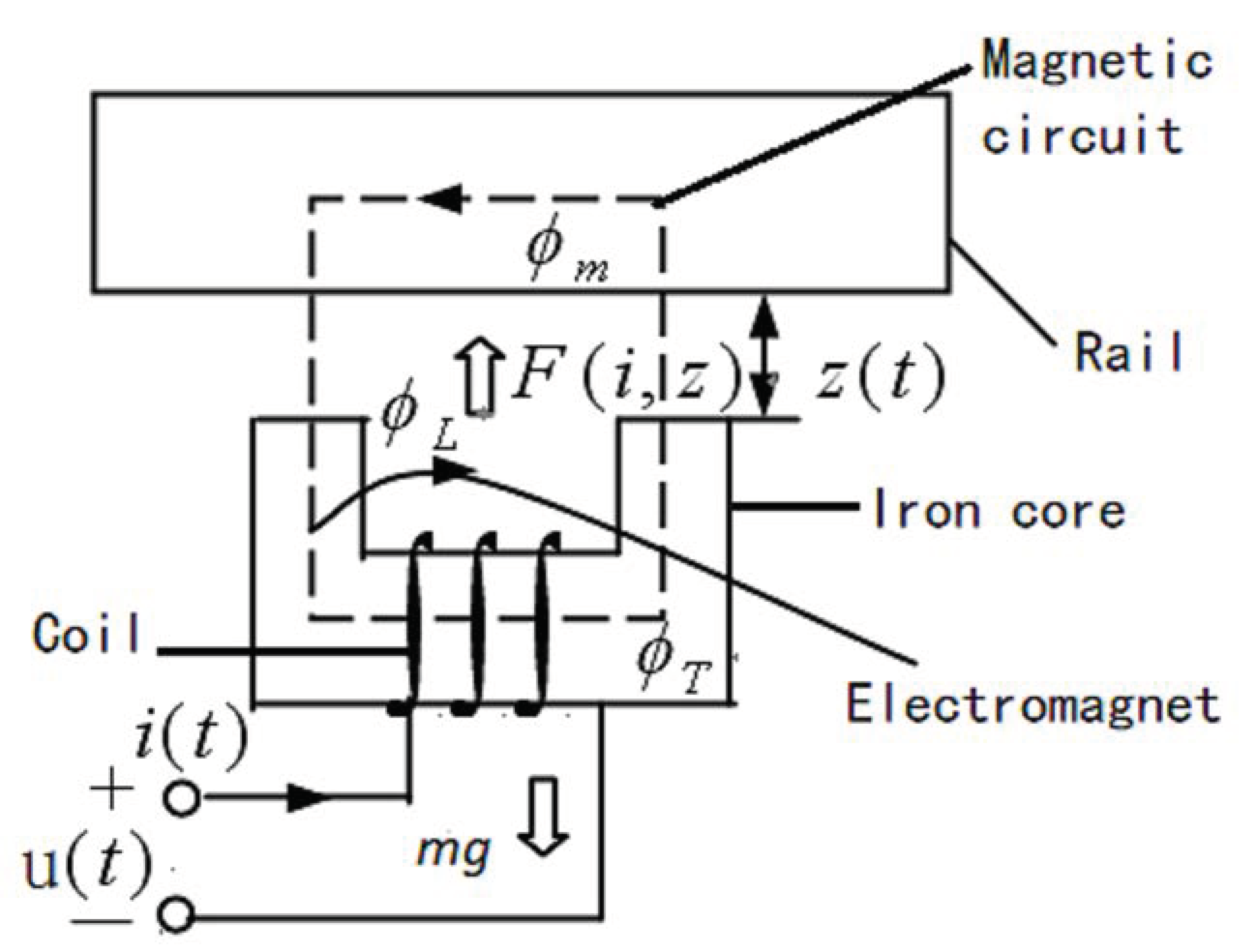
2. Maglev Levitation System Modeling

The single electromagnet levitation system is the most basic control unit in the levitation module. Although it is much easier to analyze the model and dynamic characteristics of the single electromagnet levitation system than the whole vehicle, the research and analysis of the single electromagnet is very helpful to understand the essential characteristics of the entire levitation system.

Figure 1 shows the model of the single electromagnet and rail. The relative reference dynamic model considers the motion relationship of the electromagnet relative to the track. For most laboratory-scale maglev systems, the test track is usually fixed on a structure that is much heavier than the levitation locomotive; using this model for design and analysis can obtain results with sufficient accuracy [12].

In Figure 1, ${\phi }_m$ is the air gap flux, ${\phi }_T$ is the main pole flux, ${\phi }_L$ is the leakage flux, $i\left(t\right)$ is the control current of the coil, $u\left(t\right)$ is the voltage across the control coil, $z\left(t\right)$ is the air gap between rail and electromagnet, $mg$ is the gravity of the electromagnet, $F\left(i,z\right)$ is the electromagnetic attraction force.

Besides, there are some other notations in the model. $N$ is the turns of coil, $F_m$ is the magnetic potential, $R$ is the magnetic circuit reluctance, $A$ is the cross-sectional area of iron core, $\psi$ is the air gap flux leakage.

Assumptions in the system are:

(1)

Ignore the leakage magnetic flux of the winding $\left({\phi }_L=0\right)$;

(2)

Ignore the magnetic resistance in the magnet core and the rail, that is, the magnetic potential is evenly reduced on the air gap $z\left(t\right)$;

(3)

Ignore the magnetic saturation characteristics of the materials of the track and the iron core;

(4)

The track is regarded as a rigid track; ignore elastic vibration and dynamic deformation;

(5)

The mass distribution of the entire system is uniform, and the module center coincides with the geometric center.

Then the air gap flux ${\phi }_m$ is

$${\phi }_m\approx {\phi }_T=\frac{F_m}{R_m}=\frac{Ni\left(t\right)}{2z\left(t\right)/\left({\mu }_{0}A\right)}$$

(1)

The voltage equation in the electromagnet winding circuit is

$$\begin{array}{l}u\left(t\right)=Ri\left(t\right)+\frac{d\psi }{dt}\approx Ri\left(t\right)+\frac{d}{dt}\left(N\frac{Ni\left(t\right){\mu }_{0}A}{2z\left(t\right)}\right)\\ =Ri\left(t\right)+\frac{{\mu }_0{N}^{2}A}{2z\left(t\right)}\frac{di\left(t\right)}{d\left(t\right)}-\frac{{\mu }_0{N}^{2}A}{2{[z\left(t\right)]}^2}\frac{dz\left(t\right)}{d\left(t\right)}\end{array}$$

(2)

$F\left(i,z\right)$ at any instant is

$$F\left(i,z\right)=\frac{d{W}_m}{dz}=\frac{d}{dz}{\displaystyle \int }{w}_{m}dv=\frac{d}{dz}\left(\frac{1}{2}BHV\right)=\frac{d}{dz}\left(\frac{B^{2}Az}{{\mu }_0}\right)=\frac{{\mu }_0{N}^{2}A}{4}{[\frac{i\left(t\right)}{z\left(t\right)}]}^2$$

(3)

Here, $w_m$ is the magnetic field energy density and $W_m$ is the magnetic field energy in the volume $\mathrm{V}$. Obviously, the electromagnetic attraction force $F$ and the air gap $z\left(t\right)$ have a non-linear relationship, which is the essential reason why the electromagnetic suspension system is unstable. The equation of motion of the electromagnet in the vertical direction is:

$$m\frac{d^{2}z\left(t\right)}{d{t}^2}=-F\left(i,z\right)+mg+f_d\left(t\right)$$

(4)

Here, $f_d\left(t\right)$ is the interference. In summary, the dynamics of the electromagnet suspension system is completely determined by the following equation:

$$\{\begin{array}{l}m\ddot{z}\left(t\right)=-F\left(i,z\right)+mg+f_d\left(t\right)\\ u\left(t\right)=Ri\left(t\right)+\frac{{\mu }_0{N}^{2}A}{2}\frac{i\left(t\right)}{z\left(t\right)}-\frac{{\mu }_0{N}^{2}Ai\left(t\right)}{2}\frac{\dot{z}\left(t\right)}{{[z\left(t\right)]}^2} \\ F\left(i,z\right)=\frac{{\mu }_0{N}^{2}A}{4}{[\frac{i\left(t\right)}{z\left(t\right)}]}^2\end{array}$$

(5)

Rewrite by the state variable:

$$x_1\left(t\right)=z\left(t\right),x_2\left(t\right)=\dot{z}\left(t\right),x_3\left(t\right)=i\left(t\right)$$

(6)

Then the dynamic model can be expressed as:

$$\{\begin{array}{l}{\dot{x}}_1=x_2\\ {\dot{x}}_2=-\frac{K}{m}{\left[\frac{x_3}{x_1}\right]}^2+g+\frac{f_d}{m} \\ {\dot{x}}_3=\frac{x_3{x}_2}{x_1}-\frac{R{x}_1{x}_3}{2K}+\frac{x_{1}u}{2K}\end{array}$$

(7)

Here, $K=\frac{{\mu }_0{N}^{2}A}{4}$.

3. RBF-PID Controller

The RBF network is a three-layer forward network with a single hidden layer. It simulates the neural network structure of the receptive fields, which is locally adjusted in human brain. The RBF network is a local approximation network, which has been proved to be able to approximate arbitrary continuous non-linear functions with arbitrary precision [13].

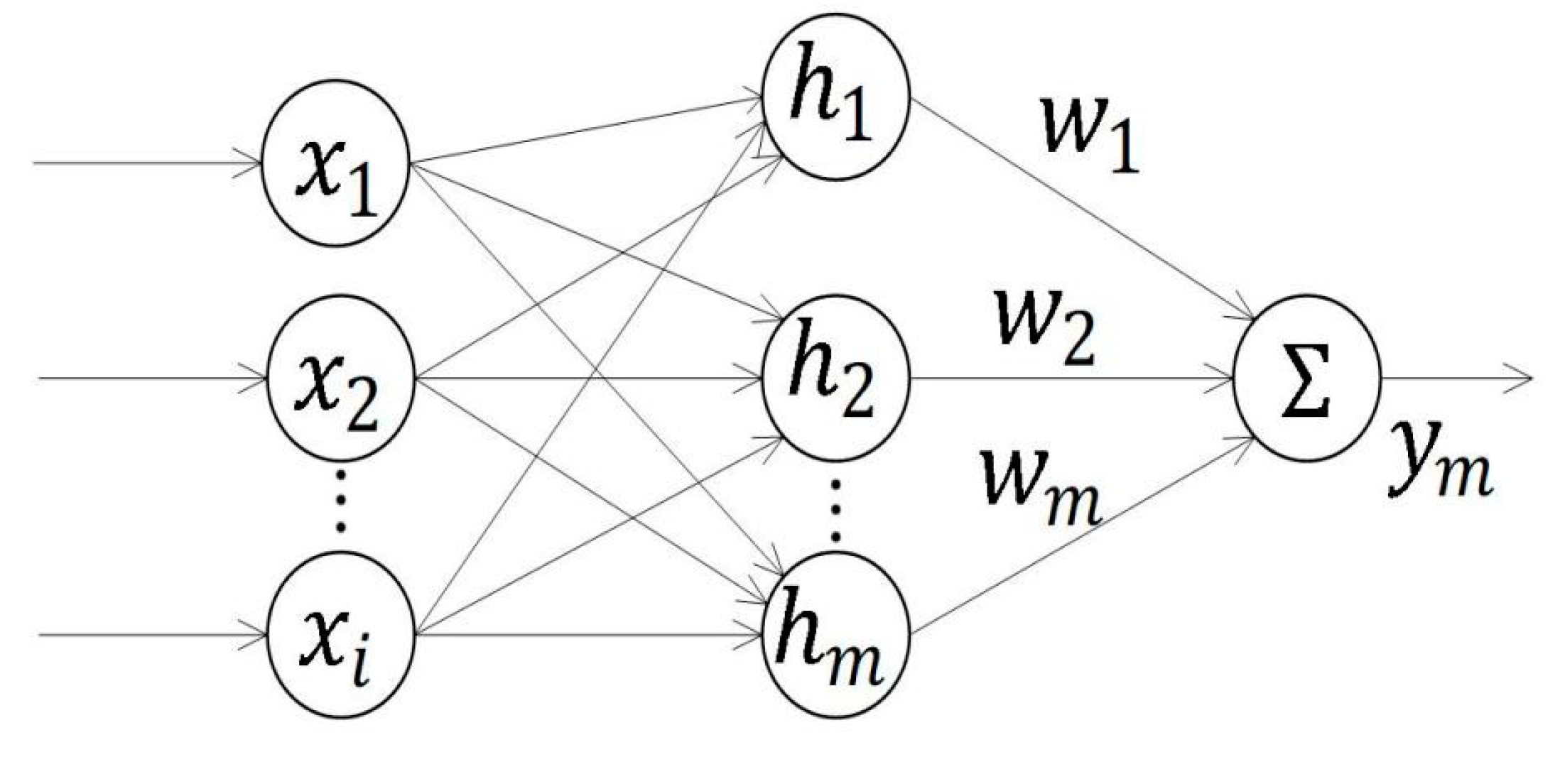
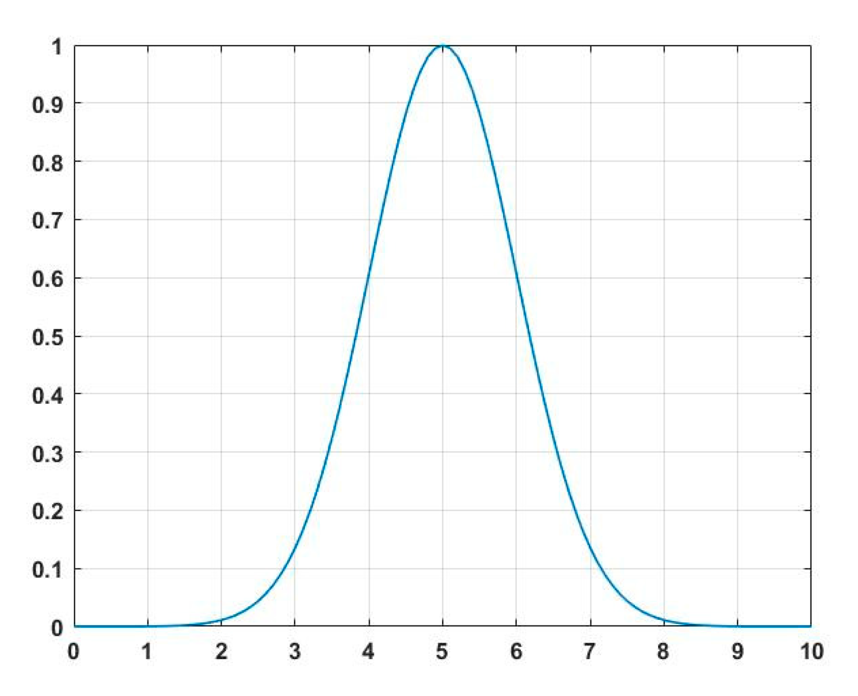
3.1. The Structure of the RBF Network

The structure of the RBF neural network includes the input layer, hidden layer and output layer. The schematic diagram is shown in Figure 2:

As is shown in Figure 2, the input of network is:

$$\mathit{x}={[x_1 x_{2 }{x}_3\dots x_i]}^T$$

(8)

The hidden layer output is:

$$\mathit{h}={[h_1 h_{2 }{h}_3\dots h_m]}^T$$

(9)

The weight of network is:

$$\mathit{w}={[w_1,w_2,\dots w_m]}^T$$

(10)

The output of network is:

$$y\left(t\right)={\mathit{w}}^{\mathit{T}}\mathit{h}=w_1{h}_1+w_2{h}_2+\dots +w_m{h}_m={\displaystyle \sum }_{j=1}^m{w}_j{h}_j$$

(11)

The activation function used in the hidden layer of the RBF network is a non-negative, non-linear function with a locally distributed center point. The performance of different activation functions in the RBF network is quite different, and the selection needs to be analyzed according to actual problems. Here, the Gaussian function (12) is selected as the activation function of the RBF network.

$$h_{j }=exp(-\frac{{\left|\right|x-c_j\left|\right|}^2}{2b_j^2})$$

(12)

The schematic diagram of the Gaussian function is shown in Figure 3.

It can be known from the expression of the Gaussian function that there are two key parameters in the Gaussian function, which are $c_j$ and $b_j$, respectively. The selection of these two parameters has certain principles as follows.

$b_j$ represents the width of the Gaussian function of the $j$th neuron in the hidden layer. The larger the value of $b_j$, the wider the Gaussian function. The width of the Gaussian function is an important factor, which has significant effect on the mapping ability of the neural network model.

$c_j$ is the coordinate vector of the center point in the Gaussian function of the $j$th neuron in the hidden layer. The closer the value of $c_j$ is to the input value, the more sensitive the Gaussian function is to the input. On the contrary, the less sensitive. It is necessary to ensure that $c_j$ is within the valid input mapping range when selected. Under normal circumstances, it is necessary to determine the coordinate vector of the center point in the Gaussian function by a certain method to ensure that the Gaussian function operates in a proper range.

In practice, the clustering method is commonly used to determine the coordinate vector$c_j$ of the center point in the Gaussian function. The clustering method is an unsupervised learning method, which is classified according to the degree of similarity between samples. By clustering the input of all samples, the center value of each node in the hidden layer is obtained. Usually the value of the $b_j$ parameter is appropriately selected and then verified.

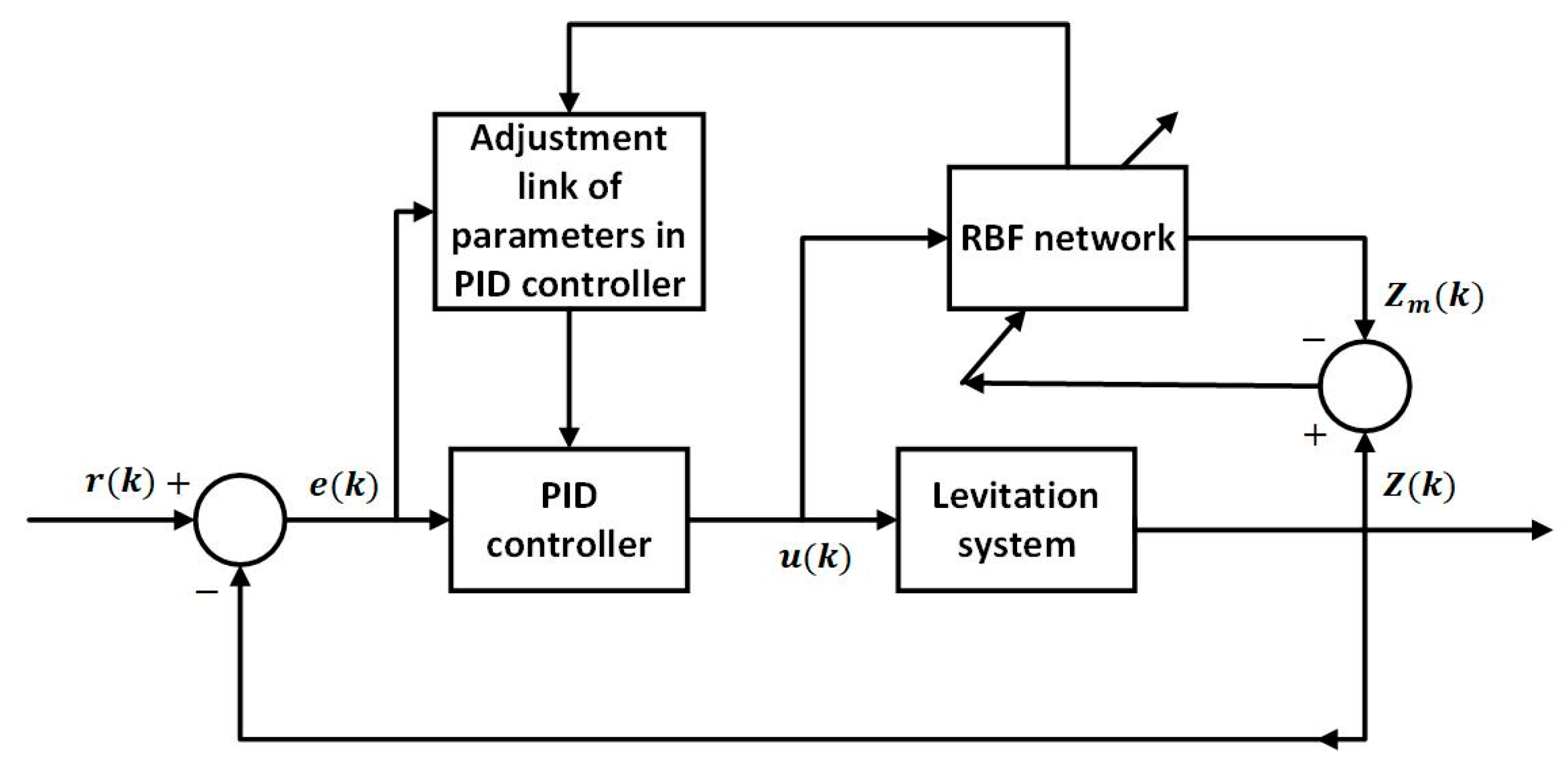
3.2. The Design of the RBF-PID Controller

The RBF network has the advantages of simple structure, fast learning speed and good real-time performance, so it can be applied to real-time control. The RBF network can be used to identify the system information, and apply the information to adjust the parameters of the PID controller online according to the actual external conditions and working status. This is the basic principle of the RBF-PID control method, which realizes self-tuning and self-adjustment of parameters in the controller according to actual information, and improves the robustness and adaptability of the system.

The RBF-PID controller of the single electromagnet levitation system is designed below. The output of the levitation system is $z$ and the output identified by the RBF network is $z_m$. The input of the RBF network recognizer is:

$$x\left(1\right)=∆u\left(k\right),x\left(2\right)=z\left(k\right),x\left(3\right)=z\left(k-1\right)$$

(13)

The structure of the RBF network is selected by the method of design first, and then test. Too many neurons will cause large computational expenses and too little neurons may not reflect the characteristics of the system properly. Therefore, we choose an appropriate number of neurons in the hidden layer first, and then the number is determined by the performance of the simulation. The final structure adopted is 3-8-1. That means the number of neurons in the hidden layer is 8, the number of neurons in the input layer is 3 and the number of neurons in the output layer is 1.

After completing the structure design of the RBF network, it is necessary to select the training method of the network parameters. Here, parameters in the RBF network use the gradient descent method with additional inertial terms for iteration.

The weight of the output $w_j$ is:

$$∆w_j=\left[z\left(k\right)-z_m\left(k\right)\right]h_j$$

(14)

$$\begin{array}{l}{w}_j\left(k\right)=w_j\left(k-1\right)+\alpha ∆w_j+\beta \left[w_j\left(k-1\right)-w_j\left(k-2\right)\right]\\ =w_j\left(k-1\right)+\alpha \left[z\left(k\right)-z_m\left(k\right)\right]h_j+\beta \left[w_j\left(k-1\right)-w_j\left(k-2\right)\right]\end{array}$$

(15)

Here, $\alpha (0<\alpha <1)$ is the learning rate. $\beta (0<\beta <1)$ is the coefficient of inertia.

The Gaussian function coordinate center of the hidden layer is:

$$∆c_{ji}=\left[z\left(k\right)-z_m\left(k\right)\right]w_j\frac{x_i-c_{ji}}{b_j^2}$$

(16)

$$\begin{array}{l}{c}_{ji}\left(k\right)=c_{ji}\left(k-1\right)+ \alpha ∆c_{ji}+ \beta \left[c_{ji}\left(k-1\right)-c_{ji}\left(k-2\right)\right]\\ =c_{ji}\left(k-1\right)+ \alpha \left[z\left(k\right)-z_m\left(k\right)\right]w_j\frac{x_i-c_{ji}}{b_j^2}\\ + \beta \left[c_{ji}\left(k-1\right)-c_{ji}\left(k-2\right)\right]\end{array}$$

(17)

The width parameter of the Gaussian function is:

$$∆b_j=\left[z\left(k\right)-z_m\left(k\right)\right]w_j{h}_j\frac{{\left|\right|x-c_j\left|\right|}^2}{b_j^3}$$

(18)

$$\begin{array}{c}{b}_j\left(k\right)=b_j\left(k-1\right)+ \alpha ∆b_j+\beta \left[b_j\left(k-1\right)-b_j\left(k-2\right)\right]\\ =b_j\left(k-1\right)+\alpha \left[z\left(k\right)-z_m\left(k\right)\right]w_j{h}_j\frac{{\left|\right|x-c_j\left|\right|}^2}{b_j^3}+\beta \left[b_j\left(k-1\right)-b_j\left(k-2\right)\right] \end{array}$$

(19)

The following is the design of the parameter adjustment link in the PID controller. The control error of the gap signal in the levitation system is:

$$e\left(t\right)=z\left(t\right)-z_0$$

(20)

Here, $z_0$ is the reference value of the gap under steady-state conditions. The output expression of the PID control method according to the current outer loop and the gap inner loop is [12]:

$$u\left(t\right)=k_C\left[k_{p}e\left(t\right)+k_i{\displaystyle \int }e\left(t\right)+k_d\dot{e}\left(t\right)-i\left(t\right)\right]$$

(21)

Here, $k_C$ is the proportional parameter of the current outer loop and $k_p$, $k_i$, $k_d$ are proportional, integral, differential parameters of the gap inner loop, respectively. $i\left(t\right)$ is the value of current in the current loop. The output of the incremental PID controller is:

$$∆u\left(t\right)=k_C\left[k_p\left[e\left(t\right)-e\left(t-1\right)\right]+k_{i}e\left(t\right)+k_d\left[\dot{e}\left(t\right)-\dot{e}\left(t-1\right)\right]-i\left(t\right)+i\left(t-1\right)\right]$$

(22)

According to the above Formula (22), we can get:

$$\frac{\partial ∆u}{\partial k_p}=k_C\left[e\left(t\right)-e\left(t-1\right)\right]$$

(23)

$$\frac{\partial ∆u}{\partial k_i}=k_C e\left(t\right)$$

(24)

$$\frac{\partial ∆u}{\partial k_d}=k_C\left[\dot{e}\left(t\right)-\dot{e}\left(t-1\right)\right]$$

(25)

Due to the large inductance of the electromagnet in the levitation system, if there is no current loop in the system, there will be a significant lag between the control voltage and the current of the electromagnet, which has a serious effect on the performance of the levitation control. The main function of current feedback is to reduce the time constant of the current loop, overcome the influence of the electromagnet inductance and ensure the response speed of the levitation system. Here, in the online adjustment of PID parameters according to the RBF network, the parameter of the current loop $k_C$ can be fixed at an appropriate value, which can reduce the difficulty of controller design.

The index performance function of the PID controller is:

$$E\left(t\right)=\frac{1}{2}{\left[z\left(t\right)-z_0\right]}^2=\frac{1}{2}{e}^2\left(t\right)$$

(26)

Then we can get:

$$\frac{\partial E}{\partial ∆u}=e\left(t\right)\frac{\partial z}{\partial ∆u}$$

(27)

Using the gradient descent method, we can get the adjustment of PID control parameters:

$$∆k_p={\alpha }_p\frac{\partial E}{\partial k_p}={\alpha }_p\frac{\partial E}{\partial ∆u}\frac{\partial ∆u}{\partial k_p}={\alpha }_{p}e\left(t\right)\frac{\partial z}{\partial ∆u}{k}_C\left[e\left(t\right)-e\left(t-1\right)\right]$$

(28)

$$∆k_i={\alpha }_i\frac{\partial E}{\partial k_i}={\alpha }_i\frac{\partial E}{\partial ∆u}\frac{\partial ∆u}{\partial k_i}={\alpha }_{i}e\left(t\right)k_C\frac{\partial z}{\partial ∆u}e\left(t\right)$$

(29)

$$∆k_d={\alpha }_d\frac{\partial E}{\partial k_d}={\alpha }_d\frac{\partial E}{\partial ∆u}\frac{\partial ∆u}{\partial k_d}={\alpha }_{d}e\left(t\right)\frac{\partial z}{\partial ∆u}{k}_C\left[\dot{e}\left(t\right)-\dot{e}\left(t-1\right)\right]$$

(30)

Here ${\alpha }_p,{\alpha }_i,{\alpha }_d$ are the learning rate factors of each parameter. $\frac{\partial z}{\partial ∆u}$ is also known as the Jacobian information of the system, using $z_m$ obtained by the RBF network identification system instead of $z$. Then we can get:

$$\frac{\partial z}{\partial ∆u}\approx \frac{\partial z_m}{\partial ∆u}=\frac{\partial \left({{\displaystyle \sum }}_{j=1}^m{w}_j{h}_j\right)}{\partial ∆u}=\frac{\partial \left({{\displaystyle \sum }}_{j=1}^m{w}_j\mathrm{e}\mathrm{x}\mathrm{p}\left(-\frac{{\left|\right|x-c_j\left|\right|}^2}{2b_j^2}\right)\right)}{\partial ∆u}={\displaystyle \sum }_{j=1}^m{w}_j{h}_j\frac{c_j-x_1}{b_j^2}$$

(31)

Because discrete control is used in the actual control, the continuous time variable of the above formula needs to be converted into discrete variables; Formula (28)–(30) can be rewritten as follows:

$$∆k_p={\alpha }_p\frac{\partial E}{\partial k_p}={\alpha }_p\frac{\partial E}{\partial ∆u}\frac{\partial ∆u}{\partial k_p}={\alpha }_{p}e\left(k\right)\frac{\partial z}{\partial ∆u}{k}_C\left[e\left(k\right)-e\left(k-1\right)\right]$$

(32)

$$∆k_i={\alpha }_i\frac{\partial E}{\partial k_i}={\alpha }_i\frac{\partial E}{\partial ∆u}\frac{\partial ∆u}{\partial k_i}={\alpha }_{i}e\left(k\right)k_C\frac{\partial z}{\partial ∆u}e\left(k\right)$$

(33)

$$∆k_d={\alpha }_d\frac{\partial E}{\partial k_d}={\alpha }_d\frac{\partial E}{\partial ∆u}\frac{\partial ∆u}{\partial k_d}={\alpha }_{d}e\left(k\right)\frac{\partial z}{\partial ∆u}{k}_C\left[\dot{e}\left(k\right)-\dot{e}\left(k-1\right)\right]$$

(34)

By adjusting the parameters of the controller through real-time signals, the changing law of each parameter in the PID controller can be obtained:

$$k_p=k_{p0}+{\alpha }_{p}e\left(k\right)\frac{\partial z}{\partial ∆u}{k}_C\left[e\left(k\right)-e\left(k-1\right)\right]$$

(35)

$$k_i=k_{i0}+{\alpha }_{i}e\left(k\right)\frac{\partial z}{\partial ∆u}{k}_{C}e\left(k\right)$$

(36)

$$k_d=k_{d0}+{\alpha }_{d}e\left(k\right)\frac{\partial z}{\partial ∆u}{k}_C\left[\dot{e}\left(k\right)-\dot{e}\left(k-1\right)\right]$$

(37)

In order to ensure the stability of the maglev system, the adjustment range of the RBF network weight is limited, so that the control parameters can be changed within an appropriate range to form a stable RBF-PID controller. Ensure that the parameters of the controller meet the requirement as follows:

$$k_{p min}\le k_p\le k_{p max}$$

(38)

$$k_{i min}\le k_i\le k_{i max}$$

(39)

$$k_{d min}\le k_d\le k_{d max}$$

(40)

Here,$k_{p min}, k_{p max}, k_{i min}, k_{i max}, k_{d min}, k_{d max}$ are the minimum and maximum boundary values of parameters that satisfy the system stability in the PID controller relatively. The specific value can be obtained experimentally.

According to the process of the controller design, the block diagram of the entire system using the RBF-PID controller is shown in Figure 4.

4. Simulation

After the design of the RBF-PID controller, a model based on the levitation system in the maglev train is established to numerically verify the effect of the controller. The parameters in the simulation system are shown in the following

Table 1. Table of parameters in single electromagnet simulation system.

Symbol	Quantity	Value
$A$	Cross-sectional area of iron core	$0.01848{ \mathrm{m}}^2$
$R_m$	Coil resistance	$0.55 \mathsf{\Omega }$
${\mu }_0$	Permeability of air	$4\pi \times {10}^{-7}$
$N$	Number of turns of coil	$360$
$M$	Quality of electromagnet system and load	$1100 \mathrm{kg}$

.

The PID method is commonly used in the control of the maglev train and has some achievements with its advantages. The research in the article mainly aims to improve the performance of the PID controller by adjusting parameters in real time with the RBF network. By comparing the experimental effects of the original PID method and the RBF-PID method, the advantages of the new method are highlighted. The initial values of the RBF-PID controller parameters remain consistent with the PID parameters. Here, the current outer loop and gap inner loop are used in the PID method as in Formula (21). Parameters of the PID controller are fixed and optimized by genetic algorithm [14].

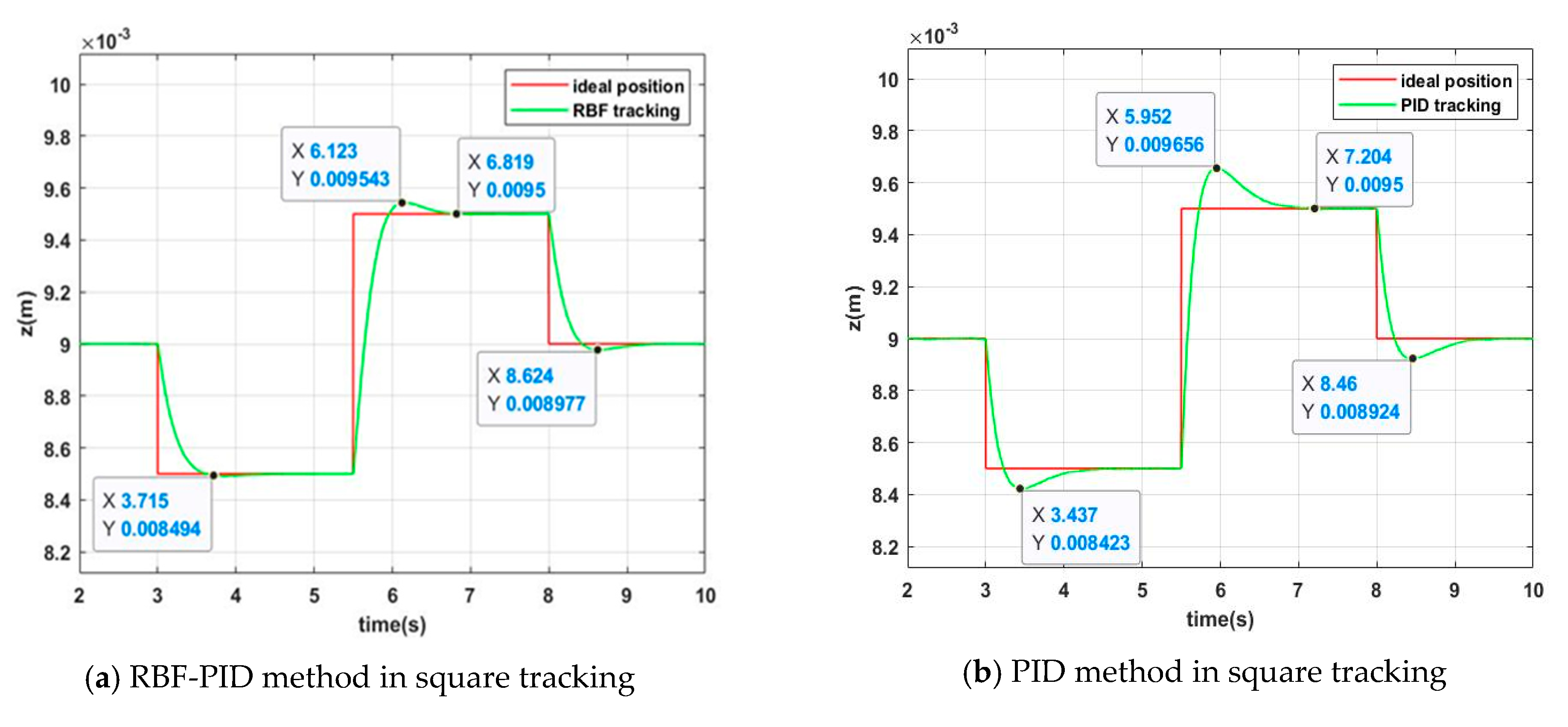
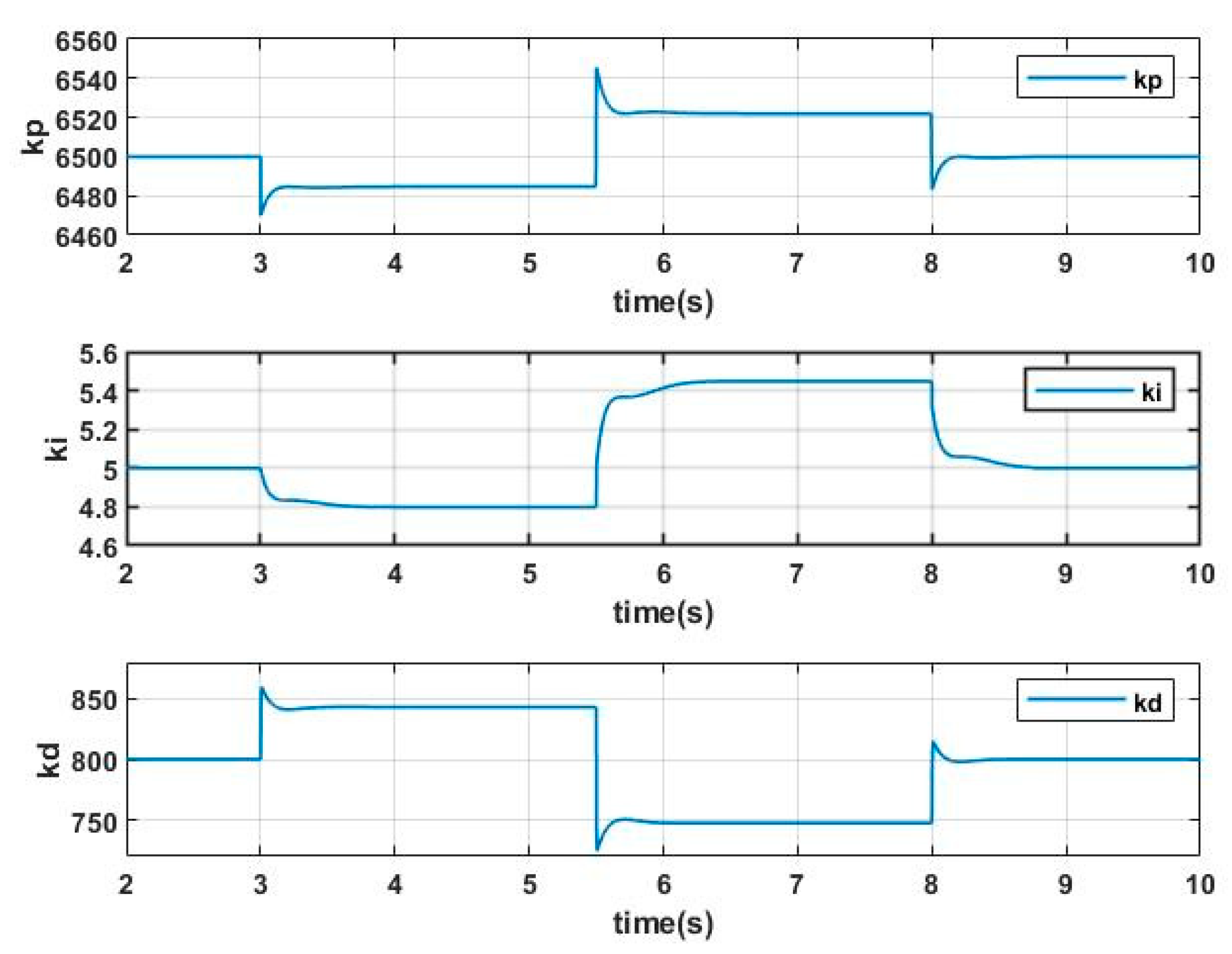
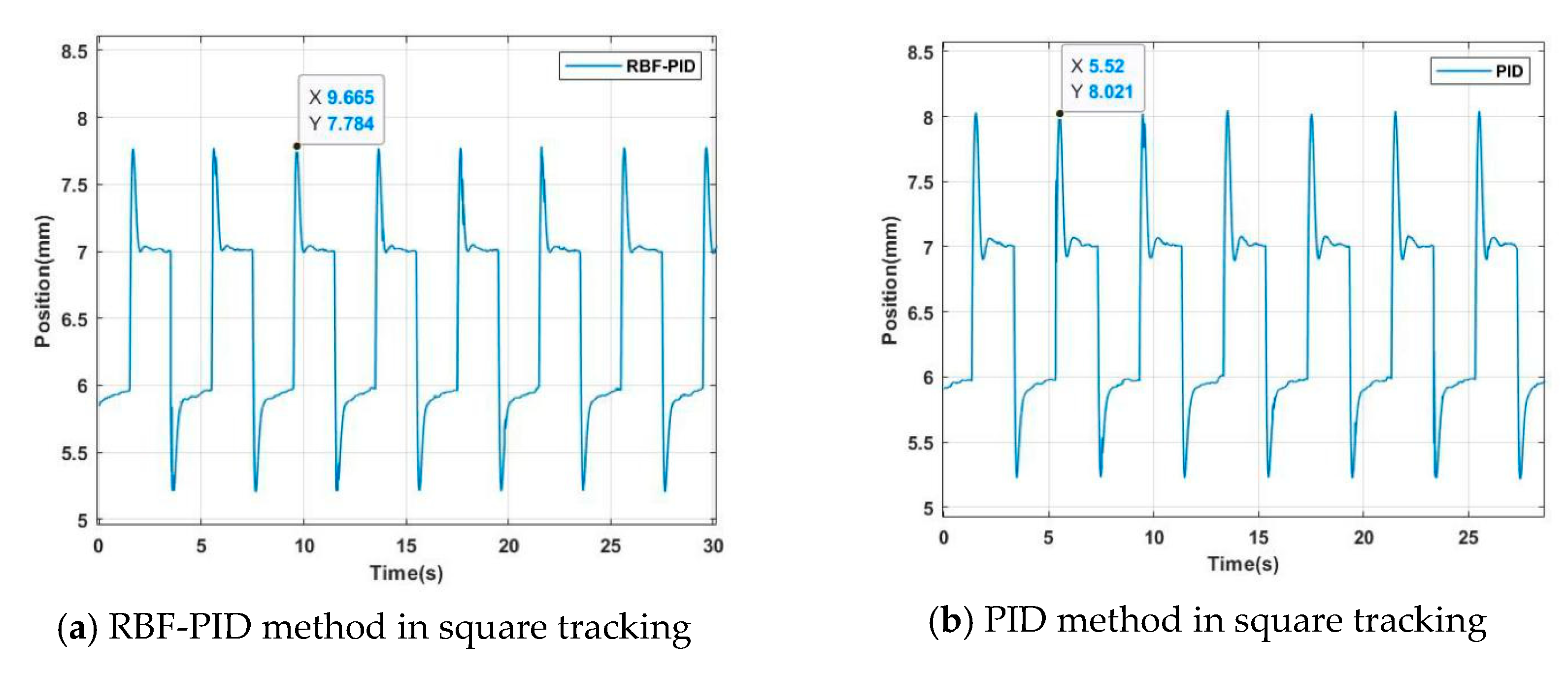
4.1. Simulation of Square Wave Tracking

Due to changes in the actual working environment, the track of the maglev train will have irregularities such as track joints, which will affect the safety and comfort of the train. This is a common external environmental interference in levitation systems, so it is necessary to ensure that the control algorithm in the levitation module has a better control effect for such situations. Here, the square wave response experiment of the levitation module is used to approximate the gap change in the track.

In the simulation, the stable gap was set at $z_0=9 \mathrm{mm}$. When the system stabilized at the equilibrium position at$t=3 \mathrm{s}$, by superimposing a square wave signal with an amplitude of $\pm 0.5 \mathrm{mm}$ and a period of $5 \mathrm{s}$ on the stable gap, the gap response of the two control methods is shown in Figure 5.

It can be seen from Figure 5 that the peak value is $9.543 \mathrm{mm}$ of the gap signal in the RBF-PID control method, which is significantly smaller than that of $9.656 \mathrm{mm}$ in the traditional PID control method, and the time for the gap signal to recover to the stable state is about $0.4 \mathrm{s}$ faster than that of the PID control method. That means when some sudden change in the track happens, the gap signal under the RBF-PID control method has a smaller fluctuation range and a shorter fluctuation time. In this case, applying the RBF-PID control method is shown to adjust the PID control parameters in real time; the levitation system has a better control effect on the change of the track than the original PID method. Figure 6 demonstrates changes of control parameters in square wave tracking of the RBF-PID method.

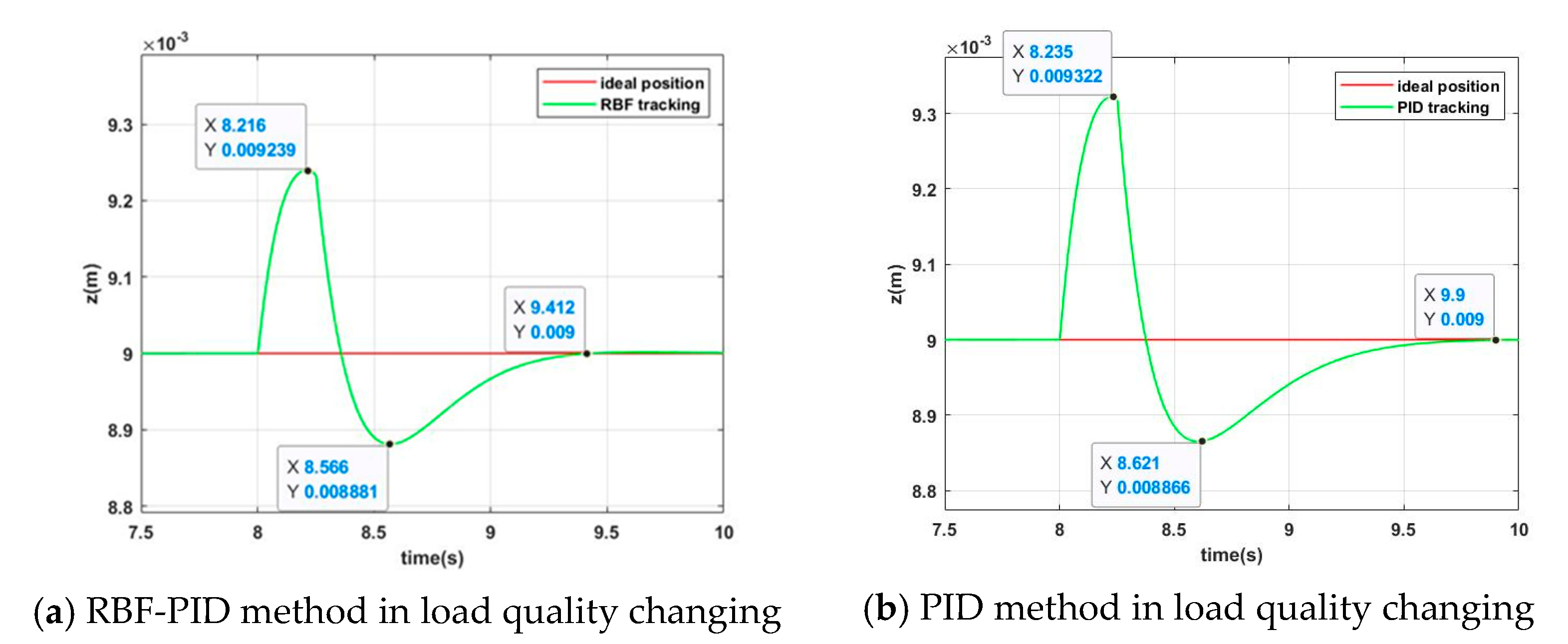
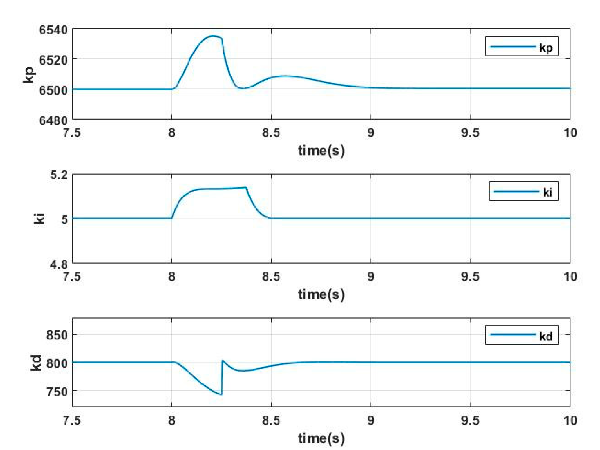
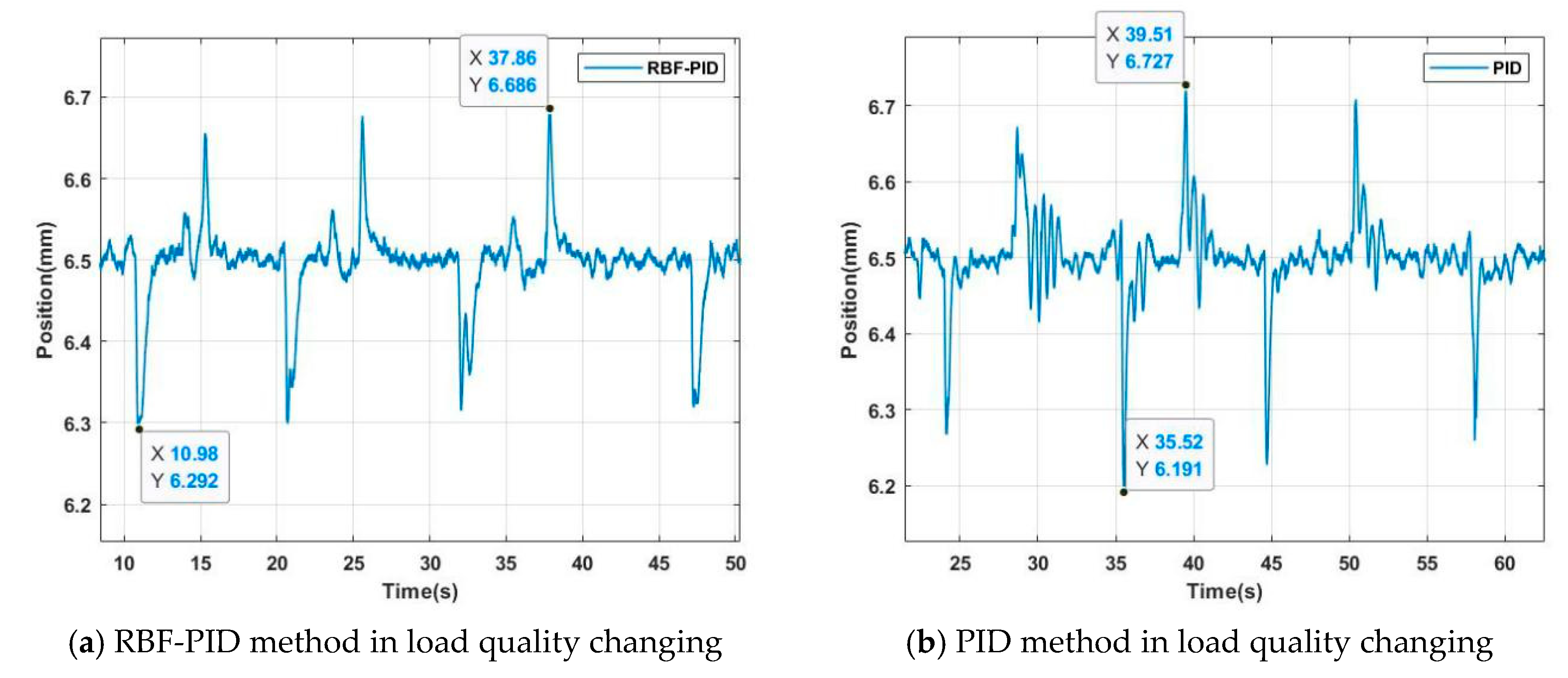
4.2. Simulation of Load Quality Changing

The maglev train is used as a means of transportation for people, and the number of passengers will cause a change of the load of the train. Actually, passengers getting on and off the vehicle bring about a sudden change in the load weight in the levitation system; this situation can be regarded as a change in the internal parameters of the system. This is in order to ensure the comfort and safety of the maglev train. The levitation system needs to have a better control effect on the change of the load quality.

In the simulation, the quality of the simulation model of the levitation system was changed from $1100 \mathrm{kg}$ to$1300 \mathrm{kg}$ at$t=8 \mathrm{s}$under the condition of stable state, and the quality was changed from $1300 \mathrm{kg}$ back to $1100 \mathrm{kg}$ at $t=8.25 \mathrm{s}$. With the actual load change on the train, the response of the levitation system is shown in Figure 7.

It can be seen from the result that the RBF-PID control method has a maximum gap fluctuation of $9.239 \mathrm{mm}$ in the case of a sudden change in system load, which is significantly smaller than the maximum fluctuation $9.322 \mathrm{mm}$ of the original PID control method, and the time it takes to return to stable state is about $0.5 \mathrm{s}$faster than the original PID control method. In the case of a sudden change in system load, the RBF-PID control method is shown to have a smaller fluctuation range and faster speed to return to the stable state. With parameter changing in the controller in real time, the control performance is improved. Figure 8 shows the changes of control parameters of the RBF-PID control method in simulation.

5. Experiments

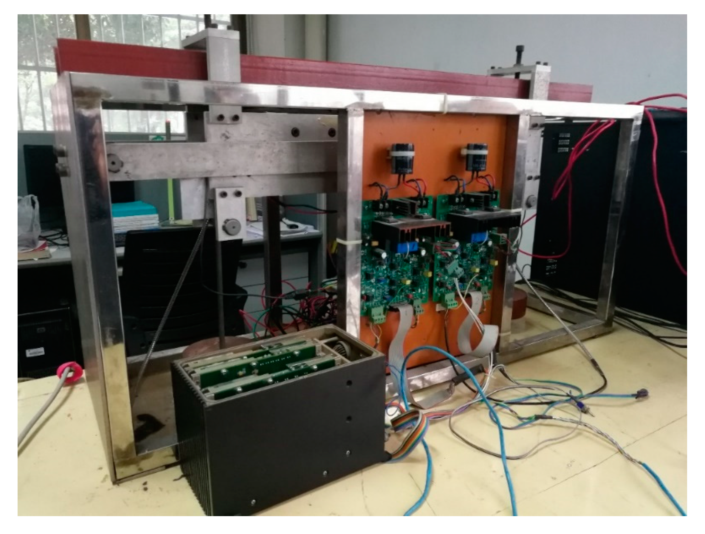
5.1. Introduction of the Small Levitation Platform

After completing the simulation of the levitation system based on the RBF-PID control method, further experiments are needed on the real levitation system to verify the effect of the control algorithm. The small levitation platform is a prototype of the levitation system in the maglev train, and the sampling frequency of the control program in the platform is 4000 Hz. It is often used for testing new control methods of the levitation system. The processor is PowerPC MPC 8260. The eddy current displacement sensor of TR 81 series is applied as the gap sensor. The power supply is −15 V and +15 V, the linear measurement range is 0~15 mm and the range of output voltage is 0~5 V. Mutual inductance current sensor is selected to measure the current signal. The range of the power supply is −15 V and +15 V, the measurement range is 0~60 A and the range of output current is 0~30 mA. The small levitation platform is shown in Figure 9.

Because the small levitation platform is a prototype of the levitation system in the maglev train, parameters of the small levitation platform are different from parameters in simulation. Parameters of the small levitation platform are shown in

Table 2. The table of parameters in the small levitation platform.

Symbol	Quantity	Value
$A$	Cross-sectional area of iron core	$0.0014{ \mathrm{m}}^2$
$R_m$	Coil resistance	$2 \mathsf{\Omega }$
$z_0$	Stable levitation gap	$6.5 \mathrm{mm}$
$N$	Number of turns of coil	$663$
$M$	Mass of electromagnet system and load	$12 \mathrm{kg}$

.

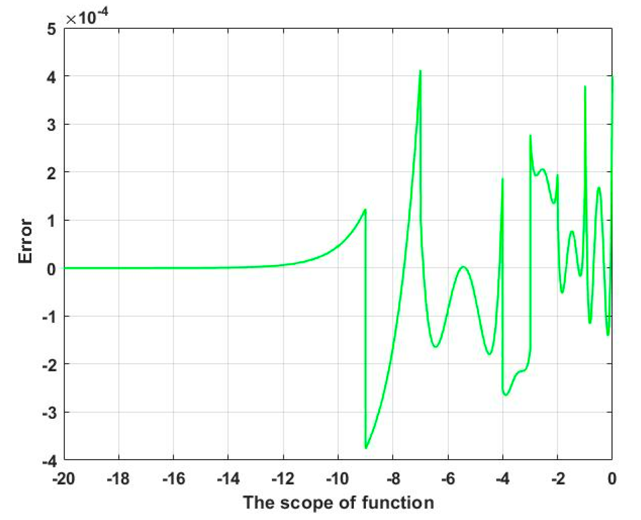
5.2. Hardware Implementation of RBF Network

Although the structure and calculation method of the RBF network are relatively simpler than other networks, there are still some difficulties in real-time control processing, especially when the dimensionality of the input data and the number of hidden layer nodes are too large—the speed of calculation cannot meet the requirement of real-time control.

As we can see in Formula (12), the Gaussian function contains an exponential function with natural logarithm as the base. In embedded systems, the processing of floating-point numbers takes up too much hardware resources and computing time. The calculation of the exponential function directly requires a longer calculation time. Generally speaking, any complex calculations can be finally converted into multiplication and addition operations. In general hardware, the basic forms of operations are multiplication and addition operations. Therefore, converting the operation in the RBF network into multiplication and addition operations can better improve the operation efficiency, and it is also necessary to ensure a certain degree of accuracy.

Therefore, the method of piecewise polynomial fitting is applied here. By dividing the function into different ranges, a simple function form is used for fitting in different ranges. Since addition and multiplication are the most basic operations in hardware, the polynomial function is used for fitting. By using the function fitting toolbox in Matlab with the principle of the least squares algorithm, the highest degree of polynomial is chosen as 3 to fit the exponential function in the Gaussian function. The specific fitting situation can be seen in

Table 3. The table of polynomial piecewise fitting function.

Range	Polynomial Function	MSE
$\left(-1,0\right)$	$y=0.1025x^3+0.4625x^2+0.9921x+0.9996$	$1.219\times {10}^{-4}$
$\left(-2,-1\right)$	$y=0.03771x^3+0.2833x^2+0.8184x+0.9405$	$4.484\times {10}^{-5}$
$\left(-3,-2\right)$	$y=0.01387x^3+0.1458x^2+0.5511x+0.7651$	$1.65\times {10}^{-5}$
$\left(-4,-3\right)$	$y=0.005103x^3+0.06896x^2+0.3252x+0.543$	$6.069\times {10}^{-6}$
$\left(-7,-4\right)$	$y=0.0007708x^3+0.01511x^2+0.1003x+0.2269$	$1.088\times {10}^{-5}$
$\left(-9,-7\right)$	$0.0004$	/
$\left(-\infty ,-9\right)$	$0$	/

.

The specific fitting error can be seen in Figure 10.

It can be seen from Figure 10 that, using the method of piecewise polynomial function for fitting, the final absolute value of the error of each point is basically less than $4\times {10}^{-4}$. It shows that the method of piecewise polynomial fitting is feasible, and the accuracy of fitting can be guaranteed. In the hardware microcomputer of the controller, each coefficient of the polynomial function used for fitting is stored in a certain data format, and can be directly called during the actual program running. The method of piecewise polynomial fitting can greatly improve the computational efficiency of the neural network in the hardware system, and ensure the real-time performance of the RBF-PID controller. Therefore, in the hardware implementation of the RBF-PID control algorithm, the exponential function in the RBF network function is replaced by the piecewise polynomial function.

5.3. Experiment of Square Wave Tracking

This is similar to the simulation, superimposing a square wave signal with an amplitude of $\pm 0.5 \mathrm{mm}$ and a period of $4 \mathrm{s}$ on the stable gap in the experiment. Figure 11 shows the gap response of two control methods; it is clearly shown that the control performance of the RBF-PID method is better in square wave tracking than that of the PID control.

5.4. Experiment of Load Quality Changing

In the experiment of load quality changing, after the system gets a stable levitation state, a 2 kg counterweight is suddenly added to the original load, and then the counterweight is removed after about 5 s, and this process is repeated a few times. Figure 12 shows the gap response of two control methods; it can be seen from the result that the fluctuation of the system in the RBF-PID method is 6.686 mm, which is smaller than 6.727 mm of the PID control.

6. Conclusions

This paper mainly discussed the application of the RBF-PID control method in the maglev system. The PID control method with fixed parameters may have poor control effect due to external interference and changes of internal parameters. Therefore, by using the ability of describing any non-linear system, the RBF network was applied in the adjustment of parameters in the controller to improve the control performance. The combination of the RBF network and the PID control can solve the control problem of the non-linear system more effectively. After completing the analysis and design of the RBF-PID controller, simulations were carried out with the model of the maglev system; the traditional PID control method was compared with the RBF-PID method. By simulating the conditions of square wave tracking and load quality changing, it was notably shown that the RBF-PID method has better control performance with parameters of controller changing in real time. Then experiments were carried out on the small levitation platform to verify the result of simulation. It was demonstrated that the RBF-PID method has a better control effect in dealing with external interference and internal parameter changing in the maglev system.

References

1. Lee, H.W.; Kim, K.C.; Lee, J. Review of maglev train technologies. IEEE Trans. Magn. 2006, 42, 1917–1925. [Google Scholar]
2. Hypiusova, M.; Osusky, J. Pid controller design for magnetic levitation model. In Proceedings of the Internation Conference, Cybernetics and Information, Vyšná Boca, Slovakia, 10–13 February 2010. [Google Scholar]
3. Ahmad, I.; Shahzad, M.; Palensky, P. Optimal PID control of magnetic levitation system using genetic algorithm. In Proceedings of the 2014 IEEE International Energy Conference (ENERGYCON), Cavtat, Croatia, 13–16 May 2014. [Google Scholar]
4. Long, Z.Q.; Hao, A.M.; Chang, W.S. Suspension controller design of maglev train considering the rail track periodical irregularity. J. Natl. Univ. Def. Technol. 2003, 25, 84–89. [Google Scholar]
5. Goodall, R.M. Dynamics and control requirements for EMS Maglev suspensions. In Proceedings of the International Conference on Maglev, Shanghai, China, 26–28 October 2004; pp. 926–993. [Google Scholar]
6. Liu, J.; Yu, L.U. Adaptive RBF neural network control of robot with actuator nonlinearities. J. Control Theory Appl. 2010, 8, 129–136. [Google Scholar] [CrossRef]
7. Junyi, L.; Xiaoming, X. Intelligent control based on neural network. Chem. Ind. Autom. Instrum. 1995, 22, 53–59. [Google Scholar]
8. Antić, D.; Milovanović, M.; Nikolić, S.; Milojković, M.; Perić, S. Simulation model of magnetic levitation based on NARX neural networks. Int. J. Intell. Syst. Appl. 2013, 5, 25–32. [Google Scholar] [CrossRef] [Green Version]
9. Suebsomran, A. Adaptive neural network control of electromagnetic suspension system. Int. J. Robot. Autom. 2014, 29, 144–154. [Google Scholar] [CrossRef]
10. Jing, Y.; Xiao, J.; Zhang, K. Compensation of gap sensor for high-speed maglev train with RBF neural network. Trans. Inst. Meas. Control 2013, 35, 933–939. [Google Scholar] [CrossRef]
11. Sun, Y.; Xu, J. Adaptive sliding mode control of maglev system based on RBF neural network minimum parameter learning method. Measurement 2018, 141, 217–226. [Google Scholar] [CrossRef]
12. Yungang, L.; Chaoxiong, K.; Hu, C. Current loop analysis and optimization design of maglev train suspension controller. J. Natl. Univ. Def. Technol. 2006, 28, 94–97. [Google Scholar]
13. Xudong, W.; Huihe, S. RBF neural network theory and its application in control. Inf. Control 1997, 26, 272–284. [Google Scholar]
14. Sun, Q.; Li, J.; Wang, H. Optimization of levitation control parameters of maglev train based on genetic algorithm. Comput. Simul. 2006, 8, 229–231. [Google Scholar]
Figure 1. Schematic diagram of single electromagnet rail model.
Symmetry 12 01780 g001
Figure 2. Schematic diagram of the radial basis function (RBF) network.
Symmetry 12 01780 g002
Figure 3. Schematic diagram of two-dimensional Gaussian function.
Symmetry 12 01780 g003
Figure 4. System block diagram of RBF-proportion integration differentiation (PID) controller.
Symmetry 12 01780 g004
Figure 5. Comparison of two control methods in square wave tracking.
Symmetry 12 01780 g005
Figure 6. Changes of control parameters in square wave tracking.
Symmetry 12 01780 g006
Figure 7. Comparison of two control methods in load quality changing.
Symmetry 12 01780 g007
Figure 8. Changes of control parameters in load quality changing.
Symmetry 12 01780 g008
Figure 9. Small levitation platform.
Symmetry 12 01780 g009
Figure 10. The graph of fitting error of piece polynomial function.
Symmetry 12 01780 g010
Figure 11. Comparison of two control methods in square wave tracking.
Symmetry 12 01780 g011
Figure 12. Comparison of two control methods in load quality changing.
Symmetry 12 01780 g012