Article

An Approach for the Global Stability of Mathematical Model of an Infectious Disease

by
Mojtaba Masoumnezhad
1,*,
Maziar Rajabi
2,
Amirahmad Chapnevis
3,
Aleksei Dorofeev
4,
Stanford Shateyi
5,*,
Narges Shayegh Kargar
6 and
Hassan Saberi Nik
7
1
Department of Mechanical Engineering, Faculty of Chamran, Guilan Branch, Technical and Vocational University (TVU), Tehran 1435761137, Iran
2
Department of Software Engineering, University of Applied Science and Technology, Shabestar, Tabriz 5164864763, Iran
3
Department of Computer Engineering and Information Technology, Amirkabir University of Technology, Tehran 1591634311, Iran
4
Head of Department of Propaedeutics of Dental Diseases, I.M. Sechenov First Moscow State Medical University, 119991 Moscow, Russia
5
Department of Mathematics, University of Venda, Private Bag X5050, Thohoyandou 0950, South Africa
6
Department of Mathematics, Payame Noor University (PNU), Tehran 193953697, Iran
7
Department of Mathematics and Statistics, University of Neyshabur, Neyshabur 9319774446, Iran
*
Authors to whom correspondence should be addressed.
Symmetry 2020, 12(11), 1778; https://doi.org/10.3390/sym12111778
Submission received: 1 August 2020 / Revised: 27 September 2020 / Accepted: 4 October 2020 / Published: 27 October 2020

Abstract

:
The global stability analysis for the mathematical model of an infectious disease is discussed here. The endemic equilibrium is shown to be globally stable by using a modification of the Volterra–Lyapunov matrix method. The basis of the method is the combination of Lyapunov functions and the Volterra–Lyapunov matrices. By reducing the dimensions of the matrices and under some conditions, we can easily show the global stability of the endemic equilibrium. To prove the stability based on Volterra–Lyapunov matrices, we use matrices with the symmetry properties (symmetric positive definite). The results developed in this paper can be applied in more complex systems with nonlinear incidence rates. Numerical simulations are presented to illustrate the analytical results.

1. Introduction

Mathematical modeling has the best predictive analysis to accurately predict the prevalence of infectious diseases, and with the help of predicting the prevalence of infection, effective strategies for disease control can be determined [1,2,3,4]. The mathematical models used for infectious diseases have evolved rapidly in recent decades. One of the reasons for this progress and development is the improvement of researchers’ ability to collect data [5,6,7,8,9,10,11].
Investigation of the global stability of endemic equilibrium in the mathematical model of infectious diseases is one of the important issues in epidemiology [12,13,14,15,16,17,18,19,20]. Several methods have been proposed by researchers to prove the stability of equilibrium points, such as monotone dynamical systems, the geometric approach, and the method of Lyapunov functions [21,22,23,24,25].
Kar and Jana presented the mathematical model of an infectious disease [26]. They examined the local and global stability of the disease free and endemic equilibrium for fixed controls. Then, they studied the optimal control of the disease with time dependent controls. For the global stability of the endemic equilibrium, Liao and Wang [27] proposed a combination of the Lyapunov function method and Volterra–Lyapunov properties and proved the global asymptotic stability of the endemic equilibria. This method does not meet the challenges of the Lyapunov function method including determining appropriate Lyapunov function and coefficients. In this work, we will present a modification of the method of Lyapunov functions combined with the theory of Volterra–Lyapunov stable matrices [27,28,29]. The fundamental difference between the two methods is that our modified method repeatedly uses Lemma 2.4, Lemma 2.8 (presented in [27]) and reducing the dimensions of the matrices, while in some parts of the original method this technique is not used. This approach transfers the analysis from differentiable functions to related matrices. The main advantage of this modification is that the higher dimensional matrices can be easily implemented. In each step, we reduce the dimensions of the matrix and use the property of the Volterra–Lyapunov matrices. This can reduce the computational complexity of the original method [27]. Furthermore, the authors in [26] used the complicated concepts and theorems to show the global stability of the endemic equilibrium. Tian and Wang in [30] investigated the global stability of the cholera epidemic models, based on the monotone dynamical systems, the geometric approach, and Volterra–Lyapunov stable matrices. The models used in their work, including different types of functions, included transmission pathways, and pathogen growth rate. Using the modified method, we can easily prove the global stability of models with nonlinear incidence rates.
The paper is organized as follows. In Section 2, we investigate the mathematical model, boundness and equilibria of model of infectious disease with fixed controls. The global stability of the endemic equilibrium is given in Section 3. In Section 4, numerical results demonstrate the effectiveness of the proposed method is presented. In this section, we have compared our modification with the original method. Finally, Section 5, contains a summarized conclusion of the results.

2. The Mathematical Model

The mathematical model of the epidemic model with two controls was proposed by Kar and Jana [26]. In this model, we have four types of population, which are represented by susceptible S ( t ) , infected I ( t ) , recovered R ( t ) and vaccinated V ( t ) .
The model consists of the following system of ordinary differential equations:
d S d t = ( 1 u 1 ) a d S λ S I 1 + α I + β R + m ( 1 ρ 1 ) I + b u 2 ( 1 ρ 2 ) I + σ V , d I d t = λ S I 1 + α I ( d + m + γ + b u 2 ) I , d R d t = ( d + β ) R + ( m ρ 1 + b u 2 ρ 2 ) I , d V d t = u 1 a ( d + σ ) V ,
The initial condition of System (1) are S ( 0 ) > 0 , I ( 0 ) > 0 , R ( 0 ) > 0 , V ( 0 ) 0 .
The used parameters of System (1) are shown in Table 1.

2.1. Equilibrium of the Model for Fixed Controls

Throughout this paper, we assume that the controls u 1 and u 2 are constant.
System (1) has two possible nonnegative equilibria. The first one is E 0 ( S 1 , 0 , 0 , V * ) where
S 1 = σ V * + ( 1 u 1 ) a d , V * = u 1 a d + σ .
This equilibrium is the disease free equilibrium. The other equilibrium is E * = ( S * , I * , R * , V * ) , where
S * = S 1 ( 1 + α I * ) R 0 , I * = S 1 ( R 0 1 ) α S 1 + ( d + γ d + m ρ 1 + b u 2 + ρ 2 ( β + d ) ) R 0 , R * = ( m ρ 1 + b u 2 ρ 2 ) I * β + d , V * = u 1 a d + σ ,
and R 0 = λ S 1 d + m + γ + b u 2 . It is easy to see that E * is feasible if I * > 0 , i.e., if R 0 = λ S 1 d + m + γ + b u 2 > 1 . The average rate of infection in susceptible individuals caused by a number of secondary infections is called the basic reproduction number R 0 .
Now, we want to get the basic reproduction number of System (1). Let us introduce matrices F and V , as follows:
F = λ S 1 0 0 0 ,
V = d + m + γ + b u 2 0 ( m ρ 1 + b u 2 ρ 2 ) d + β .
Then by applying the next generation matrix method developed by van den Driessche and Watmough [31], the basic reproduction number R 0 is the spectral radius of the next generation operator F V 1 . Thus R 0 = ρ ( F V 1 ) = λ S 1 d + m + γ + b u 2 .

2.2. Boundedness

Proposition 1.
The closed set
Γ = ( S , I , R , V ) R + 4 : 0 S + I + R + V a d ,
is positively invariant.
Proof. 
Let ( S ( t ) , I ( t ) , R ( t ) , V ( t ) ) be any solution with positive initial conditions. We have,
N ( t ) = S ( t ) + I ( t ) + R ( t ) + V ( t ) .
The time derivative of N ( t ) along the solution of (1) is
d N d t = a d S ( t ) d I ( t ) d R ( t ) d V ( t ) γ I ( t ) a d N ( t ) .
Using theory of differential equations, we get
N ( t ) a d ( 1 e d t ) + N 0 e d t ,
and for t , we have
lim t ¯ N ( t ) a d .
Hence, Γ is positively invariant and it is sufficient to consider solutions of System (1) in it. □

3. Global Stability of the Endemic Equilibrium

In this section, we are concerned with the global stability of (1) in a positively invariant set of Γ . To do this, we define the Lyapunov function as follows:
L = w 1 ( S S * ) 2 + w 2 ( I I * ) 2 + w 3 ( R R * ) 2 + w 4 ( V V * ) 2 ,
where w 1 , w 2 , w 3 and w 4 are positive constants. Calculating the time derivative of L along the trajectories of System (1), we obtain:
d L d t = 2 w 1 ( S S * ) S ˙ + 2 w 2 ( I I * ) I ˙ + 2 w 3 ( R R * ) R ˙ + 2 w 4 ( V V * ) R ˙ , = 2 w 1 ( S S * ) [ d ( S S * ) + β ( R R * ) + ( m ( 1 ρ 1 ) + b u 2 ( 1 ρ 2 ) ) ( I I * ) + σ ( V V * ) λ S I 1 + α I + λ S * I * 1 + α I * ] + 2 w 2 ( I I * ) [ ( d + m + γ + b u 2 ) ( I I * ) + λ S I 1 + α I λ S * I * 1 + α I * ] + 2 w 3 ( R R * ) [ ( d + β ) ( R R * ) + ( m ρ 1 + b u 2 ρ 2 ) ( I I * ) ] + 2 w 4 ( V V * ) [ ( d + σ ) ( V V * ) ] .
Then, we add the expression λ S * I 1 + α I into the first and second square bracket and then subtract it. As a result, we obtain
d L d t = 2 w 1 ( S S * ) [ d ( S S * ) + β ( R R * ) + ( m ( 1 ρ 1 ) + b u 2 ( 1 ρ 2 ) ) ( I I * ) + σ ( V V * ) λ S I 1 + α I + λ S * I * 1 + α I * + λ S * I 1 + α I λ S * I 1 + α I ] + 2 w 2 ( I I * ) [ ( d + m + γ + b u 2 ) ( I I * ) + λ S I 1 + α I λ S * I * 1 + α I * + λ S * I 1 + α I λ S * I 1 + α I ] + 2 w 3 ( R R * ) [ ( d + β ) ( R R * ) + ( m ρ 1 + b u 2 ρ 2 ) ( I I * ) ] + 2 w 4 ( V V * ) [ ( d + σ ) ( V V * ) ] ,
therefore, we have
d L d t = 2 w 1 ( S S * ) [ ( d + λ I 1 + α I ) ( S S * ) + β ( R R * ) + ( m ( 1 ρ 1 ) + b u 2 ( 1 ρ 2 ) λ S * ( 1 + α I ) ( 1 + α I * ) ) ( I I * ) + σ ( V V * ) ] + 2 w 2 ( I I * ) [ λ I 1 + α I ( S S * ) ( d + m + γ + b u 2 + λ S * ( 1 + α I ) ( 1 + α I * ) ) ( I I * ) ] + 2 w 3 ( R R * ) [ ( d + β ) ( R R * ) + ( m ρ 1 + b u 2 ρ 2 ) ( I I * ) ] + 2 w 4 ( V V * ) [ ( d + σ ) ( V V * ) ] ,
from where,
d L d t = 2 w 1 ( d + λ I 1 + α I ) ( S S * ) 2 + 2 w 1 β ( S S * ) ( R R * ) + 2 w 1 ( m ( 1 ρ 1 ) + b u 2 ( 1 ρ 2 ) λ S * ( 1 + α I ) ( 1 + α I * ) ) ( S S * ) ( I I * ) + 2 w 1 σ ( S S * ) ( V V * ) + 2 w 2 λ I 1 + α I ( S S * ) ( I I * ) 2 w 2 ( d + m + γ + b u 2 + λ S * ( 1 + α I ) ( 1 + α I * ) ) ( I I * ) 2
2 w 3 ( d + β ) ( R R * ) 2 + 2 w 3 ( m ρ 1 + b u 2 ρ 2 ) ( I I * ) ( R R * ) 2 w 4 ( d + σ ) ( V V * ) 2 = Y ( W A + A T W ) Y T ,
where Y = [ S S * , I I * , R R * , V V * ] , W = d i a g ( w 1 , w 2 , w 3 , w 4 ) , and
A = ( d + λ I 1 + α I ) m ( 1 ρ 1 ) + b u 2 ( 1 ρ 2 ) λ S * ( 1 + α I ) ( 1 + α I * ) β α λ I 1 + α I ( d + m + γ + b u 2 + λ S * ( 1 + α I ) ( 1 + α I * ) ) 0 0 0 m ρ 1 + b u 2 ρ 2 ( d + β ) 0 0 0 0 ( d + σ ) .
To establish the global stability of the endemic equilibrium E * , we investigate that the matrix A defined in Equation (4) is Volterra–Lyapunov stable. Below we briefly review the following prerequisites:
Here, we recall the basic definitions related to Volterra–Lyapunov stable matrices [26]. Suppose, A n × n is a real matrix.
(D1) All the eigenvalues of A have negative (positive) real parts if and only if there exists a matrix H > 0 (that is, mean H is symmetric positive definite) such that H A + A T H T < 0 ( > 0 ) [32].
(D2) The nonsingular matrix A n × n is Volterra–Lyapunov stable if there exists a positive diagonal n × n matrix M such that M A + A T M T < 0 .
(D3) The nonsingular matrix A n × n is diagonal stable (or positive stable) if there exists a positive diagonal matrix M n × n such that M A + A T M T > 0 .
(L1) [32,33]. The D = d 11 d 12 d 21 d 22 is Volterra–Lyapunov stable if and only if:
(C1-1) d 11 < 0 ,
(C1-2) d 22 < 0 ,
(C1-3) d e t ( D ) = d 11 d 22 d 12 d 21 > 0 .
(L2) [34,35]. Suppose the nonsingular D n × n = [ d i j ] , ( n 2 ) , M n × n = d i a g ( m 1 , , m n ) is a positive diagonal matrix and H = D 1 , such that:
(C2-1) d n n > 0 ,
(C2-2) M ˜ D ˜ + ( M ˜ D ˜ ) T > 0 ,
(C2-3) M ˜ H ˜ + ( M ˜ H ˜ ) T > 0 ,
it is possible to choose m n > 0 such that M D + D T M T > 0 .
Note that, D ˜ denote the ( n 1 ) × ( n 1 ) matrix obtained from D by deleting its last row and last column.
Theorem 1.
The matrix A defined in Equation (4) is Volterra–Lyapunov stable.
Proof. 
Clearly A 44 > 0 . Let us consider D = A ˜ , denote the 3 × 3 matrix obtained from A by deleting its last row and last column. From Equation (4), we obtain
D = A ˜ = ( d + λ I 1 + α I ) m ( 1 ρ 1 ) b u 2 ( 1 ρ 2 ) + λ S * ( 1 + α I ) ( 1 + α I * ) β λ I 1 + α I ( d + m + γ + b u 2 + λ S * ( 1 + α I ) ( 1 + α I * ) ) 0 0 m ρ 1 b u 2 ρ 2 ( d + β ) .
Based on (L2), we state and prove the following results. The first Lemma, proves that D = A ˜ is diagonal stable and in the next Lemma, we show the H = A 1 ˜ is diagonal stable. Therefore, all the conditions of (L2) are satisfied. Hence the matrix A is Volterra–Lyapunov stable. □
Lemma 1.
The matrix D defined in Equation (5), is diagonal stable.
Proof. 
Let’s now discuss the diagonal stability of D. It is guaranteed by the following steps:
Step 1. 
It is obvious that D 33 > 0 .
Step 2. 
By using (L2), we shall prove that the matrix D ˜ is diagonal stable. From (5), we obtain
D ˜ = ( d + λ I 1 + α I ) m ( 1 ρ 1 ) b u 2 ( 1 ρ 2 ) + λ S * ( 1 + α I ) ( 1 + α I * ) λ I 1 + α I ( d + m + γ + b u 2 + λ S * ( 1 + α I ) ( 1 + α I * ) ) .
Obviously, D ˜ 11 > 0 , and D ˜ 22 > 0 . It remains to show that d e t ( D ˜ ) > 0 :
d e t ( D ˜ ) = d ( d + m + γ + b u 2 + λ S * ( 1 + α I ) ( 1 + α I * ) ) + λ I 1 + α I ( m + b u 2 ) + λ I 1 + α I ( d + γ + λ S * ( 1 + α I ) ( 1 + α I * ) ) λ I 1 + α I ( m + b u 2 ) + λ I 1 + α I ( m ρ 1 + b u 2 ρ 2 + λ S * ( 1 + α I ) ( 1 + α I * ) ) ,
then we have
d e t ( D ˜ ) = d ( d + m + γ + b u 2 + λ S * ( 1 + α I ) ( 1 + α I * ) ) + λ I 1 + α I ( d + γ + λ S * ( 1 + α I ) ( 1 + α I * ) ) + λ I 1 + α I ( m ρ 1 + b u 2 ρ 2 + λ S * ( 1 + α I ) ( 1 + α I * ) ) > 0 ,
therefore D ˜ is diagonal stable.
Step 3. 
Now, we must show that D 1 ˜ is diagonal stable. Let us consider the D 1 as following:
D 1 = d 11 d 12 d 13 d 21 d 22 d 23 d 31 d 32 d 33 ,
where,
d 11 = ( d + β ) [ d + m + γ + b u 2 + λ S * ( 1 + α I ) ( 1 + α I * ) ] , d 12 = ( d + β ) [ m ( 1 ρ 1 ) + b u 2 ( 1 ρ 2 ) λ S * ( 1 + α I ) ( 1 + α I * ) ] + β ( m ρ 1 + b u 2 ρ 2 ) , d 13 = β ( d + m + γ + b u 2 + λ S * ( 1 + α I ) ( 1 + α I * ) ) , d 21 = λ I 1 + α I ( d + β ) ,
d 22 = ( d + λ I 1 + α I ) ( d + β ) , d 23 = β λ I 1 + α I , d 31 = λ I 1 + α I ( m ρ 1 + b u 2 ρ 2 ) , d 32 = ( d + λ I 1 + α I ) ( m ρ 1 + b u 2 ρ 2 ) , d 33 = d ( d + m + γ + b u 2 + λ S * ( 1 + α I ) ( 1 + α I * ) ) + λ I 1 + α I ( m + γ + m ρ 1 + b u 2 ρ 2 ) + 2 λ I 1 + α I ( λ S * ( 1 + α I ) ( 1 + α I * ) ) .
Now, we have D 1 ˜ as:
D 1 ˜ = 1 d e t ( D ) ( d + β ) [ d + m + γ + b u 2 + λ S * ( 1 + α I ) ( 1 + α I * ) ] ( d + β ) [ m ( 1 ρ 1 ) + b u 2 ( 1 ρ 2 ) λ S * ( 1 + α I ) ( 1 + α I * ) ] + β ( m ρ 1 + b u 2 ρ 2 ) λ I 1 + α I ( d + β ) ( d + λ I 1 + α I ) ( d + β ) .
Following some calculations, we obtain that
d e t ( D ) = d ( d + β ) ( m + b u 2 ) + ( d + β ) ( d + λ I 1 + α I ) ( d + γ + λ S * ( 1 + α I ) ( 1 + α I * ) ) + d λ I 1 + α I ( m ρ 1 + b u 2 ρ 2 ) + ( d + β ) ( λ I 1 + α I ) λ S * ( 1 + α I ) ( 1 + α I * ) ) > 0 ,
Then
d e t ( D 1 ˜ ) = 1 ( d e t ( D ) ) 2 d ( d + β ) 2 ( d + m + γ + b u 2 + λ S * ( 1 + α I ) ( 1 + α I * ) ) + 1 ( d e t ( D ) ) 2 ( d + β ) 2 ( λ I 1 + α I ) ( d + γ + λ S * ( 1 + α I ) ( 1 + α I * ) ) + 1 ( d e t ( D ) ) 2 ( d + β ) 2 ( λ I 1 + α I ) ( λ S * ( 1 + α I ) ( 1 + α I * ) ) + 1 ( d e t ( D ) ) 2 d ( d + β ) ( λ I 1 + α I ) ( m ρ 1 + b u 2 ρ 2 ) > 0 .
It is easy to see, D 1 ˜ 11 > 0 and D 1 ˜ 22 > 0 . Therefore, D 1 ˜ is diagonal stable. □
Lemma 2.
The matrix H = A 1 ˜ is diagonal stable.
Proof. 
We can obtain the A 1 ˜ as following:
H = ( A 1 ˜ ) = 1 d e t ( A ) e 11 e 12 e 13 e 21 e 22 e 23 e 31 e 32 e 33 ,
where,
e 11 = ( d + β ) ( d + σ ) ( d + β ) 2 ( d + m + γ + b u 2 + λ S * ( 1 + α I ) ( 1 + α I * ) ) , e 12 = ( d + β ) ( d + σ ) ( m + b u 2 ) d ( d + σ ) ( m ρ 1 + b u 2 ρ 2 + λ S * ( 1 + α I ) ( 1 + α I * ) ) β ( d + σ ) ( λ S * ( 1 + α I ) ( 1 + α I * ) ) , e 13 = β ( d + σ ) ( d + m + γ + b u 2 + λ S * ( 1 + α I ) ( 1 + α I * ) ) , e 21 = ( d + β ) ( d + σ ) ( λ I 1 + α I ) , e 22 = ( d + β ) ( d + σ ) ( d + λ I 1 + α I ) , e 23 = β ( d + σ ) ( λ I 1 + α I ) , e 31 = ( d + σ ) ( m ρ 1 + b u 2 ρ 2 ) , e 32 = ( d + σ ) ( d + λ I 1 + α I ) ( m ρ 1 + b u 2 ρ 2 ) , e 33 = d ( d + m + γ + b u 2 + λ S * ( 1 + α I ) ( 1 + α I * ) ) , ( d + σ ) ( λ I 1 + α I ) ( d + γ + m ρ 1 + b u 2 ρ 2 + 2 λ S * ( 1 + α I ) ( 1 + α I * ) ) .
It is obvious that H 33 > 0 . Below, we show H ˜ and H 1 ˜ are diagonally stable.
H ˜ = 1 d e t ( A ) e 11 e 12 e 21 e 22 .
First, we show that d e t ( A ) > 0 :
d e t ( A ) = d ( d + β ) ( d + σ ) ( d m + γ + b u 2 + λ S * ( 1 + α I ) ( 1 + α I * ) ) ( d + β ) ( d + σ ) ( λ I 1 + α I ) ( d + γ + λ S * ( 1 + α I ) ( 1 + α I * ) ) + d λ I 1 + α I ( d + σ ) ( m ρ 1 + b u 2 ρ 2 + λ S * ( 1 + α I ) ( 1 + α I * ) ) + β λ I 1 + α I ( d + σ ) ( λ S * ( 1 + α I ) ( 1 + α I * ) ) > 0 .
Also, we can show that d e t ( H ˜ ) > 0 (see the Appendix A).
It remains to show that H 1 ˜ is diagonal stabe. Define
H 1 ˜ = 1 d e t ( H ) h 11 h 12 h 21 h 22 .
The h 11 is writen as
h 11 = d ( d + β ) ( d + σ ) 2 ( d m + γ + b u 2 + λ S * ( 1 + α I ) ( 1 + α I * ) ) ( d + λ I 1 + α I ) + d ( d + σ ) 2 ( d + λ I 1 + α I ) ) λ I 1 + α I ) ( d + γ + m ρ 1 + b u 2 ρ 2 + 2 λ S * ( 1 + α I ) ( 1 + α I * ) ) + β ( d + σ ) 2 ( d + λ I 1 + α I ) ) λ I 1 + α I ) ( d + γ + 2 λ S * ( 1 + α I ) ( 1 + α I * ) ) > 0 .
The h 22 is writen as
h 22 = d ( d + β ) ( d + σ ) 2 ( d + m + γ + b u 2 + λ S * ( 1 + α I ) ( 1 + α I * ) ) 2 + d ( d + σ ) 2 ( d + λ I 1 + α I ) ) λ I 1 + α I ) ( d + γ + m ρ 1 + b u 2 ρ 2 + 2 λ S * ( 1 + α I ) ( 1 + α I * ) ) + β ( d + σ ) 2 λ I 1 + α I ) ( d + γ + 2 λ S * ( 1 + α I ) ( 1 + α I * ) ) ( d + m + γ + b u 2 + λ S * ( 1 + α I ) ( 1 + α I * ) ) > 0 .
It is easy to see d e t ( H ) > 0 , see the Appendix B. Therefore, H 1 ˜ is diagonal stable. □
Summarizing the above discussions, we have the following conclusions for the globally asymptotically stablity of the endemic equilibrium.
Theorem 2.
When R 0 > 1 , the endemic equilibrium E * = ( S * , I * , R * , V * ) , of Model (1) is globally asymptotically stable, in Γ.
Proof. 
Lemmas 1 and 2 with the aid of Theorem 1, guarantee that the endemic equilibrium of the model System (1) is globally asymptotically stable. □

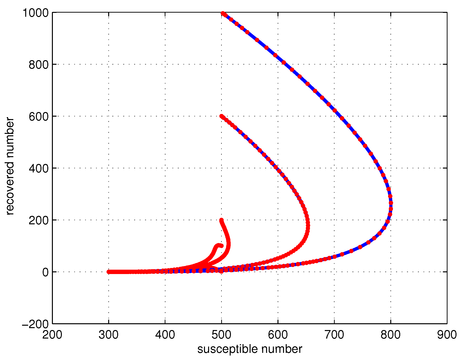
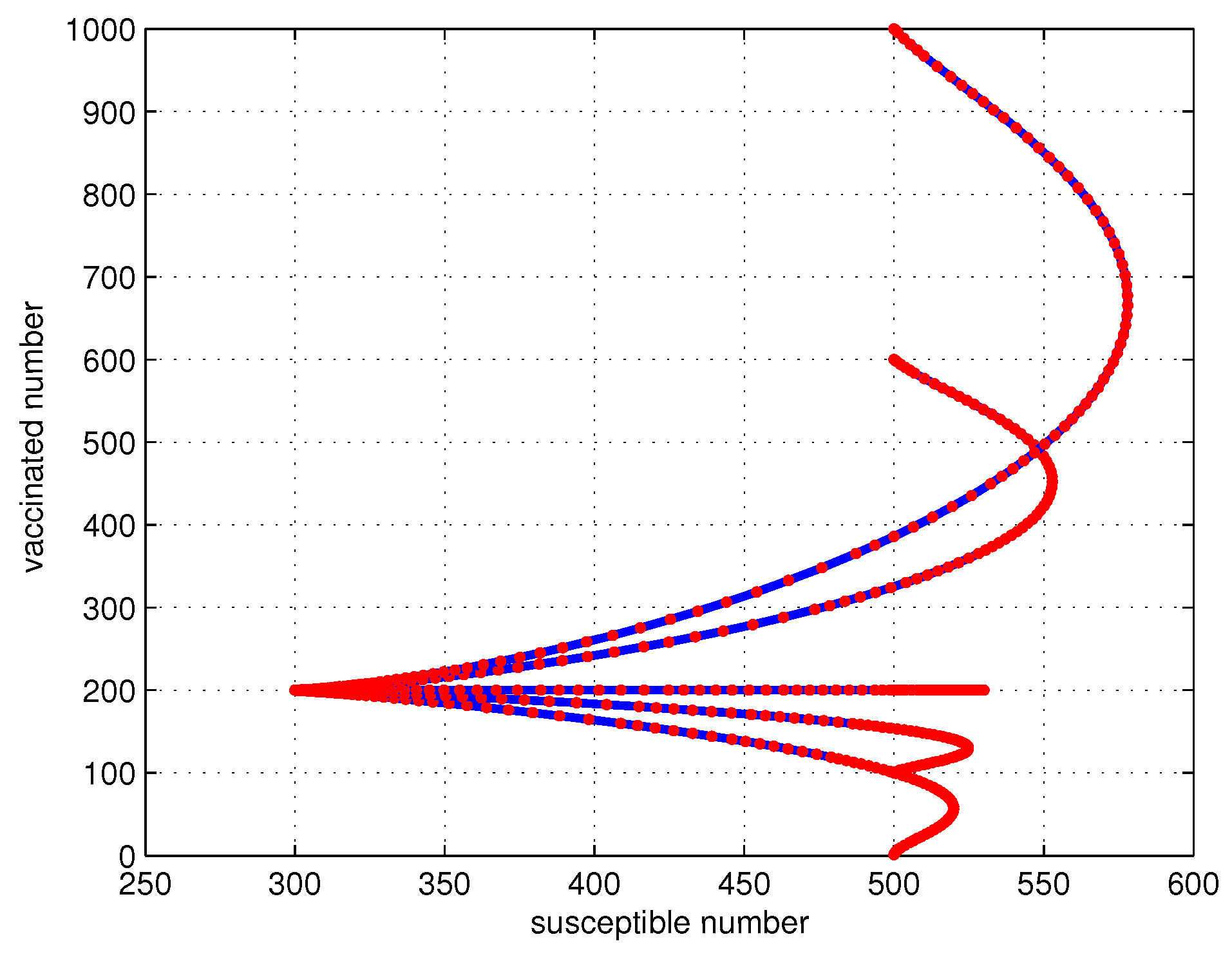
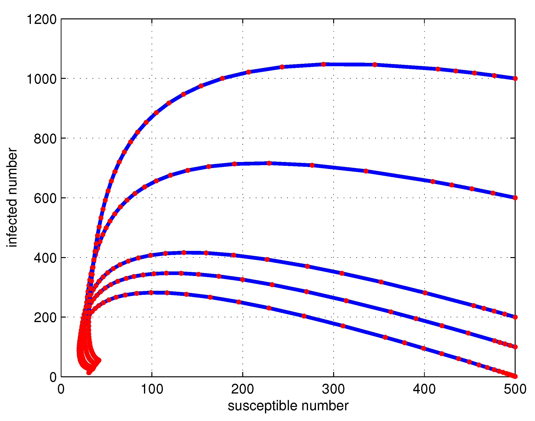
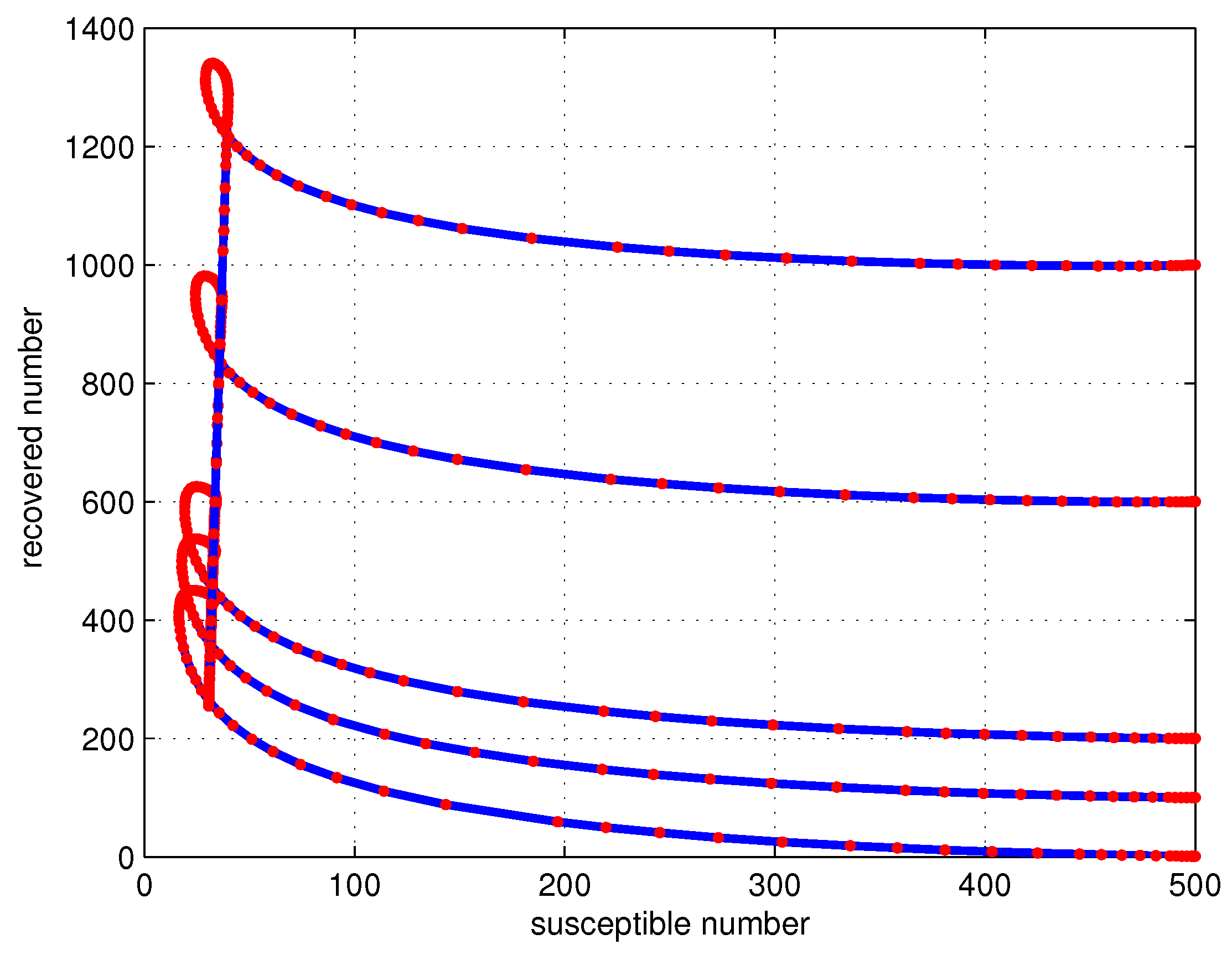
4. Numerical Simulations and Discussion

In this section, we present some numerical simulations of System (1) using the basic reproduction number R 0 , to support the analytical results. Parameters were taken from [26].

4.1. Simulations

Example 1.
We choose the parameter values as follows: a = 100 ,   d = 0.2 ,   λ = 0.01 ,   β = 0.4 ,   σ = 0.05 ,   m = 0.8 ,   ρ 1 = 0.78 ,   ρ 2 = 0.93 ,   γ = 0.02 ,   α = 0.01 ,   u 1 = u 2 = 0.5 ,   b = 15 .
With the mentioned parameters, System (1) has only a disease-free equilibrium point of E 0 = ( 300 , 0 , 0 , 200 ) . In this case, the basic reproduction number is less than one. The phase diagram is demonstrated in Figure 1, at different initial values I ( 0 ) = 1 , 100 , 200 , 600 , 1000 , to validate the stability of the disease free equilibrium at I = 0 , S = 300 . In Figure 2, we observe that the five orbits converge to the E 0 at R = 0 , S = 300 , with five different initial conditions R ( 0 ) = 1 , 100 , 200 , 600 , 1000 . In Figure 3, there are five solution curves corresponding to initial conditions with V ( 0 ) = 1 , 100 , 200 , 600 , 1000 , which ensures the stability of the disease free equilibrium at V = 200 , S = 300 .
Example 2.
For System (1), we choose the parameter values as follows: a = 100 ,   d = 0.2 ,   λ = 0.5 ,   β = 0.4 ,   σ = 0.05 ,   m = 5.8 ,   ρ 1 = 0.78 ,   ρ 2 = 0.93 ,   γ = 0.02 ,   α = 0.01 ,   u 1 = u 2 = 0.5 ,   b = 15 .
System (1) has two equilibria; one is disease free and the other is endemic equilibrium E * ( 30 , 13.3 , 255 , 200 ) . It can easily verified that R 0 > 1 . The phase diagram of System (1) at different initial values I ( 0 ) = 1 , 100 , 200 , 600 , 1000 , shown in Figure 4, which shows that all system responses converge to point of E * at I = 13.3 ,   S = 30 . In Figure 5, we see that five orbits converge to the E * at R = 255 ,   S = 30 , at different initial conditions R ( 0 ) = 1 , 100 , 200 , 600 , 1000 . In Figure 6, there are five solution curves corresponding to initial conditions with V ( 0 ) = 1 , 100 , 200 , 600 , 1000 , which proves the stability of the disease-free equilibrium point at V = 200 ,   S = 30 .

4.2. Discussion

The authors in [27], applied the original method for proving the global stability of endemic equilibrium of the system of three-dimensional and four-dimensional. At first, they define D = A and E = ( A ) 1 , to discuss the Volterra–Lyapunov stability of A 3 × 3 . Hence, following the steps they concluded that A 3 × 3 is a Volterra–Lyapunov stable matrix:
  • Showing that E is stable, based on (L1).
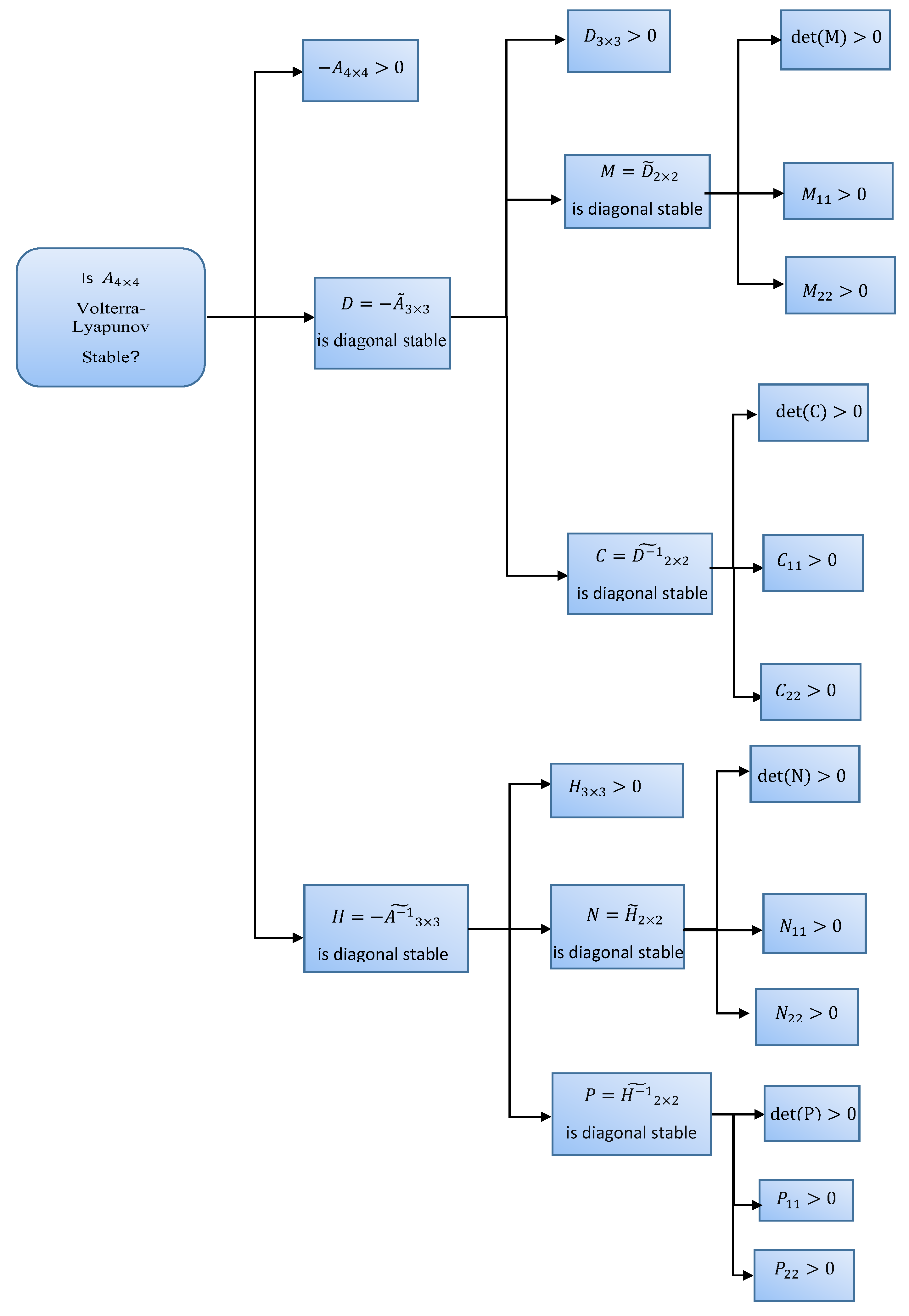
  • To prove that D is Volterra–Lyapunov stable, they performed another process. Defined
    W ˜ E ˜ + ( W ˜ E ˜ ) T = 1 d e t A Q > 0 , W ˜ D ˜ + ( W ˜ D ˜ ) T = P ,
    where, Q 2 × 2 is positive. Finally, by some algebraic and matrix manipulations, showed that P 2 × 2 > 0 .
    To compare the results in this paper with the original method, the process of proving the stability of matrix A 4 × 4 is shown in Figure 7. According to our investigations on different systems, and as the authors mentioned in Section 6 [27], the implementation of the method for the higher dimensions systems (in the second step proposed by the authors) is very difficult and complex. Therefore, the use of the modified method, can reduce the complexity of the calculations.
Based on Figure 7, by decreasing the size of the matrix A 4 × 4 to A ˜ 3 × 3 , applying (L2), finally reducing to 2 × 2 matrix, and using (L1), it can easily be proved that A is a Volterra–Lyapunov stable matrix.

5. Conclusions

We have investigated the global stability of the endemic equilibrium point of an infectious disease model. In this paper, using the modified Volterra–Lyapunov matrices method, the stability of the model has been analyzed. The main advantage of this modification is its application to various systems of epidemics, infection diseases and even chaotic dynamical systems. This leads to better performance and reduces the complexity of the proofs. The numerical results verify the effectiveness of the proposed scheme.

Author Contributions

M.M., M.R., A.C., and A.D., contributed equally to conceptualization, formal analysis and writing—original draft preparation; S.S., N.S.K., H.S.N. contributed equally to methodology, software, and numerical simulation. All authors have read and agreed to the published version of the manuscript.

Funding

This research received no external funding.

Conflicts of Interest

The authors declare that there is no conflict of interests regarding the publication of this article.

Appendix A

Proof of  d e t ( H ˜ ) > 0 : 
Let
a 11 a 22 = d ( d + β ) 2 ( d + σ ) 2 ( d + m + γ + b u 2 + λ S * ( 1 + α I ) ( 1 + α I * ) ) + ( d + β ) 2 ( d + σ ) 2 ( λ I 1 + α I ) ( m + b u 2 ) + ( d + β ) 2 ( d + σ ) 2 ( λ I 1 + α I ) ( d + γ + λ S * ( 1 + α I ) ( 1 + α I * ) ) ,
and
a 12 a 21 = d ( d + β ) 2 ( d + σ ) 2 ( m + b u 2 ) d ( d + β ) ( d + σ ) 2 ( λ I 1 + α I ) ( m ρ 1 + b u 2 ρ 2 + λ S * ( 1 + α I ) ( 1 + α I * ) ) β ( d + β ) ( d + σ ) 2 ( λ I 1 + α I ) ( λ S * ( 1 + α I ) ( 1 + α I * ) ) .
Therefore, we have
d e t ( H ˜ ) = ( 1 d e t ( A ) ) 2 ( a 11 a 22 a 12 a 21 ) = d ( d + β ) 2 ( d + σ ) 2 ( d + m + γ + b u 2 + λ S * ( 1 + α I ) ( 1 + α I * ) ) + ( d + β ) 2 ( d + σ ) 2 ( λ I 1 + α I ) ( d + γ + λ S * ( 1 + α I ) ( 1 + α I * ) ) + d ( d + β ) ( d + σ ) 2 ( λ I 1 + α I ) ( m ρ 1 + b u 2 ρ 2 + λ S * ( 1 + α I ) ( 1 + α I * ) ) + β ( d + β ) ( d + σ ) 2 ( λ I 1 + α I ) ( λ S * ( 1 + α I ) ( 1 + α I * ) ) .
Hence, it is clear to see d e t ( H ˜ ) > 0 . The proof is then complete.

Appendix B

Proof of  d e t ( H ) > 0 : 
The d e t ( H ) is written as
( 1 d e t ( A ) ) 3 [ a 11 ( a 22 a 33 a 23 a 32 ) a 21 ( a 12 a 33 a 13 a 32 ) + a 31 ( a 12 a 23 a 13 a 22 ) ] .
It is easy to see that a 21 a 13 a 32 a 31 a 13 a 22 = 0 , hence we show that
a 11 a 22 a 33 a 11 a 23 a 32 a 21 a 12 a 33 + a 31 a 12 a 23 > 0 .
To this end, we have
a 11 a 22 a 33 = d ( d + β ) 2 ( d + σ ) 2 ( d + λ I 1 + α I ) ( d + m + γ + b u 2 + λ S * ( 1 + α I ) ( 1 + α I * ) ) 2 + ( d + β ) 2 ( d + σ ) 2 ( λ I 1 + α I ) ( d + λ I 1 + α I ) ( d + γ + λ S * ( 1 + α I ) ( 1 + α I * ) ) ( d + γ + m ρ 1 + b u 2 ρ 2 + 2 λ S * ( 1 + α I ) ( 1 + α I * ) ) ,
and
a 11 a 23 a 32 = β ( d + σ ) 3 ( d + β ) ( m ρ 1 + b u 2 ρ 2 ) ( λ I 1 + α I ) ( d + λ I 1 + α I ) ( d + m + γ + b u 2 + λ S * ( 1 + α I ) ( 1 + α I * ) ) ,
and
a 21 a 12 a 33 = ( d + σ ) 3 ( d + β ) 2 ( m + b u 2 ρ 2 ) ( λ I 1 + α I ) ( d + m + γ + b u 2 + λ S * ( 1 + α I ) ( 1 + α I * ) ) d 2 ( d + σ ) 3 ( d + β ) ( λ I 1 + α I ) ( m ρ 1 + b u 2 ρ 2 + λ S * ( 1 + α I ) ( 1 + α I * ) ) ( d + m + γ + b u 2 + λ S * ( 1 + α I ) ( 1 + α I * ) ) β d ( d + σ ) 3 ( d + β ) 2 ( λ I 1 + α I ) ( λ S * ( 1 + α I ) ( 1 + α I * ) ) ( d + m + γ + b u 2 + λ S * ( 1 + α I ) ( 1 + α I * ) ) + ( d + σ ) 3 ( d + β ) ( λ I 1 + α I ) 2 ( m + b u 2 ) ( d + γ + m ρ 1 + b u 2 ρ 2 + 2 λ S * ( 1 + α I ) ( 1 + α I * ) ) d ( d + σ ) 3 ( d + β ) ( λ I 1 + α I ) 2 ( m ρ 1 + b u 2 ρ 2 + λ S * ( 1 + α I ) ( 1 + α I * ) ) ) ( d + γ + m ρ 1 + b u 2 ρ 2 + 2 λ S * ( 1 + α I ) ( 1 + α I * ) ) β ( d + σ ) 3 ( d + β ) ( λ I 1 + α I ) 2 ( λ S * ( 1 + α I ) ( 1 + α I * ) ) ( d + γ + m ρ 1 + b u 2 ρ 2 + 2 λ S * ( 1 + α I ) ( 1 + α I * ) ) ,
also
a 31 a 12 a 23 = β ( d + σ ) 3 ( d + β ) ( λ I 1 + α I ) 2 ( m ρ 1 + b u 2 ρ 2 ) ( m + b u 2 ) β d ( d + σ ) 3 ( λ I 1 + α I ) 2 ( m ρ 1 + b u 2 ρ 2 ) ( m ρ 1 + b u 2 ρ 2 + λ S * ( 1 + α I ) ( 1 + α I * ) ) , β 2 ( d + σ ) 3 ( λ I 1 + α I ) 2 ( m ρ 1 + b u 2 ρ 2 ) ( λ S * ( 1 + α I ) ( 1 + α I * ) ) .
Hence, it is clear to see d e t ( H ) > 0 . The proof is then complete.

References

  1. Anderson, R.M.; May, R.M. Infectious Diseases of Humans: Dynamics and Control; Oxford University Press: Oxford, UK, 1991. [Google Scholar]
  2. Hethcote, H.W. The mathematics of infectious diseases. SIAM Rev. 2000, 42, 599–653. [Google Scholar] [CrossRef] [Green Version]
  3. Korobeinikov, A. Global properties of basic virus dynamics models. Bull. Math. Biol. 2004, 66, 879–883. [Google Scholar] [CrossRef] [PubMed]
  4. Abouelkheir, I.; Kihal, F.E.; Rachik, M.; Elmouki, I. Time needed to control an epidemic with restricted resources in SIR model with short-term controlled population: A fixed point method for a free isoperimetric optimal control problem. Math. Comput. Appl. 2018, 23, 64. [Google Scholar] [CrossRef] [Green Version]
  5. Hethcote, H.W.; Van Den Driessche, P. Some epidemiological models with nonlinear incidence. J. Math. Biol. 1991, 29, 271–287. [Google Scholar] [CrossRef] [PubMed] [Green Version]
  6. Zhao, Y.; Li, M.; Yuan, S. Analysis of Transmission and Control of Tuberculosis in Mainland China, 2005–2016, Based on the Age-Structure Mathematical Model. Int. J. Environ. Res. Public Health 2017, 14, 1192. [Google Scholar] [CrossRef] [Green Version]
  7. Agaba, G.O.; Kyrychko, Y.N.; Blyuss, K.B. Time-delayed SIS epidemic model with population awareness. Ecol. Complex. 2017, 31, 50–56. [Google Scholar] [CrossRef] [Green Version]
  8. Sen, M.D.; Ibeas, A.; Quesada, S.A.; Nistal, R. On a SIR model in a patchy environment under constant and feedback decentralized controls with asymmetric parameterizations. Symmetry 2019, 11, 430. [Google Scholar] [CrossRef] [Green Version]
  9. Bairagi, N.; Adak, D. Role of precautionary measures in HIV epidemics: A mathematical assessment. Int. J. Biomath. 2016, 9, 1650096. [Google Scholar] [CrossRef]
  10. Sayan, M.; Hıncal, E.; Sanlıdag, T.; Kaymakamzade, B.; Saad, F.T.; Baba, I.A. Dynamics of HIV/AIDS in Turkey from 1985 to 2016. Qual. Quant. 2018, 52, 711–723. [Google Scholar] [CrossRef]
  11. Liu, X.; Takeuchi, Y.; Iwami, S. SVIR epidemic models with vaccination strategies. J. Theor. Biol. 2008, 253, 1–11. [Google Scholar] [CrossRef]
  12. Ma, Y.; Liu, J.B.; Li, H. Global dynamics of an SIQR model with vaccination and elimination hybrid strategies. Mathematics 2018, 6, 328. [Google Scholar] [CrossRef] [Green Version]
  13. Upadhyay, R.K.; Pal, A.K.; Kumari, S.; Roy, P. Dynamics of an SEIR epidemic model with nonlinear incidence and treatment rates. Nonlinear Dyn. 2019, 96, 2351–2368. [Google Scholar] [CrossRef]
  14. Mwasa, A.; Tchuenche, J.M. Mathematical analysis of a cholera model with public health interventions. BioSystems 2011, 105, 190–200. [Google Scholar] [CrossRef]
  15. Wang, L.; Xu, R. Global stability of an SEIR epidemic model with vaccination. Int. J. Biomath. 2016, 9, 1650082. [Google Scholar] [CrossRef]
  16. Bentaleb, D.; Amine, S. Lyapunov function and global stability for a two-strain SEIR model with bilinear and nonmonotone incidence. Int. J. Biomath. 2019, 12, 1950021. [Google Scholar] [CrossRef]
  17. Chen, X.; Cao, J.; Park, J.H.; Qiu, J. Stability analysis and estimation of domain of attraction for the endemic equilibrium of an SEIQ epidemic model. Nonlinear Dyn. 2017, 87, 975–985. [Google Scholar] [CrossRef]
  18. Baba, I.A.; Hincal, E. Global stability analysis of two-strain epidemic model with bilinear and non-monotone incidence rates. Eur. Phys. J. Plus 2017, 132, 208. [Google Scholar] [CrossRef]
  19. Geng, Y.; Xu, J. Stability preserving NSFD scheme for a multi-group SVIR epidemic model. Math. Methods Appl. Sci. 2017, 40, 4917–4927. [Google Scholar] [CrossRef]
  20. Zaman, G.; Kang, Y.H.; Jung, I.H. Stability analysis and optimal vaccination of an SIR epidemic model. BioSystems 2008, 93, 240–249. [Google Scholar] [CrossRef]
  21. Yi, L.; Liu, Y.; Yu, W. Combination of Improved OGY and Guiding Orbit Method for Chaos Control. J. Adv. Comput. Intell. Intell. Inf. 2019, 23, 847–855. [Google Scholar] [CrossRef]
  22. Wang, X.; Liu, X.; Xie, W.C.; Xu, W.; Xu, Y. Global stability and persistence of HIV models with switching parameters and pulse control. Math. Comput. Simul. 2016, 123, 53–67. [Google Scholar] [CrossRef]
  23. Hu, Z.; Ma, W.; Ruan, S. Analysis of SIR epidemic models with nonlinear incidence rate and treatment. Math. Biosci. 2012, 238, 12–20. [Google Scholar] [CrossRef]
  24. Misra, A.K.; Sharma, A.; Shukla, J.B. Stability analysis and optimal control of an epidemic model with awareness programs by media. BioSystems 2015, 138, 53–62. [Google Scholar] [CrossRef] [PubMed]
  25. Thieme, H.R. Global stability of the endemic equilibrium in infinite dimension: Lyapunov functions and positive operators. J. Differ. Equ. 2011, 250, 3772–3801. [Google Scholar] [CrossRef] [Green Version]
  26. Kar, T.K.; Jana, S. A theoretical study on mathematical modelling of an infectious disease with application of optimal control. BioSystems 2013, 111, 37–50. [Google Scholar] [CrossRef] [PubMed]
  27. Liao, S.; Wang, J. Global stability analysis of epidemiological models based on Volterra-Lyapunov stable matrices. Chaos Solitons Fractals 2012, 45, 966–977. [Google Scholar] [CrossRef]
  28. Parsaei, M.R.; Javidan, R.; Shayegh Kargar, N.; Saberi Nik, H. On the global stability of an epidemic model of computer viruses. Theory Biosci. 2017, 136, 169–178. [Google Scholar] [CrossRef]
  29. Zahedi, M.S.; Kargar, N.S. The Volterra-Lyapunov matrix theory for global stability analysis of a model of the HIV/AIDS. Int. J. Biomath. 2016, 10, 1750002. [Google Scholar] [CrossRef]
  30. Tian, J.P.; Wang, J. Global stability for cholera epidemic models. Math. Biosci. 2011, 232, 31–41. [Google Scholar] [CrossRef]
  31. Driessche, V.D.; Watmough, J. Reproduction numbers and sub-threshold endemic equilibria for compartmental models of disease transmission. Math. Biosci. 2002, 180, 29–48. [Google Scholar] [CrossRef]
  32. Cross, G.W. Three types of matrix stability. Linear Algebra Appl. 1978, 20, 253–263. [Google Scholar] [CrossRef] [Green Version]
  33. Rinaldi, F. Global stability results for epidemic models with latent period. IMA J. Math. Appl. Med. Biol. 1990, 7, 69–75. [Google Scholar] [CrossRef]
  34. Redheffer, R. Volterra multipliers I. SIAM J. Algebr. Discret. Methods 1985, 6, 592–611. [Google Scholar] [CrossRef]
  35. Redheffer, R. Volterra multipliers II. SIAM J. Algebr. Discret. Methods 1985, 6, 612–623. [Google Scholar] [CrossRef]
Figure 1. The phase portraits of I vs. S for System (1), with initial conditions I ( 0 ) = 1 , 100 , 200 , 600 , 1000 , ( R 0 < 1 ).
Symmetry 12 01778 g001
Figure 2. The phase portraits of R vs. S for System (1), with initial conditions R ( 0 ) = 1 , 100 , 200 , 600 , 1000 , ( R 0 < 1 ).
Symmetry 12 01778 g002
Figure 3. The phase portraits of V vs. S for System (1), with initial conditions V ( 0 ) = 1 , 100 , 200 , 600 , 1000 , ( R 0 < 1 ).
Symmetry 12 01778 g003
Figure 4. The phase portraits of I vs. S for System (1), with initial conditions I ( 0 ) = 1 , 100 , 200 , 600 , 1000, ( R 0 > 1 ).
Symmetry 12 01778 g004
Figure 5. The phase portraits of R vs. S for System (1), with initial conditions R ( 0 ) = 1 , 100 , 200 , 600 , 1000, ( R 0 > 1 ).
Symmetry 12 01778 g005
Figure 6. The phase portraits of V vs. S for System (1), with initial conditions V ( 0 ) = 1 , 100 , 200 , 600 , 1000, ( R 0 > 1 ).
Symmetry 12 01778 g006
Figure 7. All steps of proving Volterra–Lyapunov stability of matrix A 4 × 4 using the modified method.
Symmetry 12 01778 g007
Table 1. The parameters of System (1).
ParameterDescription
aThe total recruitment
u 1 The constant vaccination control
σ Transmission rates from vaccinated to susceptible
α The reciprocal of half-saturation
λ The infection force parameter
λ S I 1 + α I The saturated infection rate
mInfected population rate that have recovered naturally
ρ 1 The portion recovered ( 0 < ρ 1 < 1 )
u 2 The constant treatment control
bThe effectiveness of the treatment
b u 2 The rate by which the infected populations recovered
β R The part of the recovered class becomes susceptible
ρ 2 Recovered sections that go to recovery class ( 0 < ρ 2 < 1 )
γ Death rate of infected people due to disease attack
dThe natural death rate
Publisher’s Note: MDPI stays neutral with regard to jurisdictional claims in published maps and institutional affiliations.

