Article

Genetic Algorithm Based on Natural Selection Theory for Optimization Problems

1
CAIT, Faculty of Information Science and Technology, Universiti Kebangsaan Malaysia, Bangi 43600, Malaysia
2
School of Electrical Engineering, Department of Communication Engineering, Universiti Teknologi Malaysia, UTM Johor Bahru, Johor 81310, Malaysia
*
Author to whom correspondence should be addressed.
Symmetry 2020, 12(11), 1758; https://doi.org/10.3390/sym12111758
Submission received: 29 August 2020 / Revised: 30 September 2020 / Accepted: 5 October 2020 / Published: 23 October 2020
(This article belongs to the Section Computer)

Abstract

:
The metaheuristic genetic algorithm (GA) is based on the natural selection process that falls under the umbrella category of evolutionary algorithms (EA). Genetic algorithms are typically utilized for generating high-quality solutions for search and optimization problems by depending on bio-oriented operators such as selection, crossover, and mutation. However, the GA still suffers from some downsides and needs to be improved so as to attain greater control of exploitation and exploration concerning creating a new population and randomness involvement happening in the population at the solution initialization. Furthermore, the mutation is imposed upon the new chromosomes and hence prevents the achievement of an optimal solution. Therefore, this study presents a new GA that is centered on the natural selection theory and it aims to improve the control of exploitation and exploration. The proposed algorithm is called genetic algorithm based on natural selection theory (GABONST). Two assessments of the GABONST are carried out via (i) application of fifteen renowned benchmark test functions and the comparison of the results with the conventional GA, enhanced ameliorated teaching learning-based optimization (EATLBO), Bat and Bee algorithms. (ii) Apply the GABONST in language identification (LID) through integrating the GABONST with extreme learning machine (ELM) and named (GABONST-ELM). The ELM is considered as one of the most useful learning models for carrying out classifications and regression analysis. The generation of results is carried out grounded upon the LID dataset, which is derived from eight separate languages. The GABONST algorithm has the capability of producing good quality solutions and it also has better control of the exploitation and exploration as compared to the conventional GA, EATLBO, Bat, and Bee algorithms in terms of the statistical assessment. Additionally, the obtained results indicate that (GABONST-ELM)-LID has an effective performance with accuracy reaching up to 99.38%.

1. Introduction

The past few decades have witnessed an increasing interest in using nature-inspired algorithms to solve numerous optimization problems including timetabling problems [1,2,3,4]; data mining [5,6,7]; breast cancer diagnosis [8]; load balancing of tasks in cloud computing [9]; language identification [10,11]; and vehicle routing problems [12,13,14]. The observation of processes found in nature became the basis for nature-inspired algorithms of which the main objective is to seek the global optimal solutions for certain problems [15]. There are two common key factors in nature-inspired algorithms, namely diversification (exploration) and intensification (exploitation). Exploration entails the search for global optima via the random exploration of new solution spaces; meanwhile, exploitation entails the search for local optima in solution spaces that have been previously explored [15]. Optimal solution is not found via intense exploration, while algorithm is trapped in local optima due to deep exploitation [15]. Hence, a balance between both factors is pertinent for any nature-inspired algorithm [15,16].
Numerous nature-inspired algorithms have been suggested in literature such as particle swarm optimization [17]; genetic algorithm [18]; bat algorithm [19]; harmony search [20]; and kidney-inspired algorithm [21]. Physical/biological activities found in the natural world form the basis for nature-inspired algorithms in the quest to find solutions for various optimization problems [21], which then render these algorithms to be effective optimization algorithms. Nevertheless, shortcomings including finding the balance between the key factors of exploration and exploitation could still be prevalent, which affects the algorithm’s efficacy [15,21].
Among these metaheuristics, the genetic algorithm (GA) is considered as one of the most popular metaheuristic algorithms that has been used in practically all optimization, design and application areas [11]. GA is actually one of the earliest proposed population-based stochastic algorithms. GA consists of the selection, crossover, and mutation operations, similar to other evolutionary algorithms (EAs). Darwin’s theory of evolution [22,23,24], i.e., the survival of the fittest, makes up the basis of GA whereby the fittest genes are simulated. Its algorithm is population-based, and each solution matches a chromosome whilst each parameter denotes a gene. A fitness (objective) function is used to evaluate the fitness of each individual in the population. For improving poor solutions, the best solutions are chosen randomly with a selection (e.g., random, k-tournament or roulette wheel) mechanism. This operator is more likely to choose the best solutions since the probability is proportional to the fitness (objective value). What increases local optima avoidance is the probability of choosing poor solutions. This means that if good solutions are trapped in a local solution, they can be pulled out with other solutions.
Despite its proven capacity in resolving numerous search and optimization problems [25], GA still has several weaknesses. For example, in GA, the mechanism of both 1: the new population is generated from the existing parents and 2: the randomness involvement that happened in the population at the time of solution initialization may both lead to making the GA fail to create exploration in the solution search space. In addition, the mutation is applied to the new chromosomes (offspring) that are obtained from the crossover operation and then moved to the next generation (using same pool) that might lead to not providing a good enough exploration and solution diversity. In other words, the crossover followed by mutation may prevent the mutation and crossover operations from guaranteeing an optimal solution [26,27,28]. Hence, this current study proposes a new GA based on the theory of natural selection to improve the GA performance. The proposed genetic algorithm based on natural selection theory (GABONST) has been evaluated based on the following: (i) fifteen renowned benchmark test functions (ii) apply the GABONST in language identification (LID) through integrating the GABONST with extreme learning machine (ELM) (GABONST-ELM) and compare the proposed GABONST-ELM with enhanced self-adjusting extreme learning machine (ESA-ELM) algorithm. The ESA-ELM is based on enhanced ameliorated teaching learning-based optimization (EATLBO) [29], where EATLBO still suffers from some downsides in terms of the selection criteria and the ability to create good fresh solutions. The explanation of the new proposed GABONST is provided in Section 2.2.
A reminder that this paper is organized as such: Section 2 presents the proposed method. Section 3 details the experiments carried out and their respective findings, and finally Section 4 presents the general conclusions and suggestions for future research.

2. Materials and Methods

2.1. Genetic Algorithm

The concept of GA is aimed to imitate the natural changes that occur in living ecosystems, which is social systems, evaluate the psychological consequences, and model the variable methods. Holland [30] pointed out that Goldberg [22] had significantly contributed to the widespread usage of GA by demonstrating that a large number of problems can basically be solved by utilizing the GA methods. According to [31,32], GA is a widely popular search and optimization method for resolving highlyintricate problems. The success of its methods has been proven in areas involving machine learning approaches. A complete description of the actual coded GA is provided in this section. Figure 1 provides the flowchart of the standard GA.
Below is the description of the standard GA procedure [33]:
Initial population. This entails the possible solution for set P, i.e., a series of random generations of real values, P = {p1, p2, …, ps}.
Evaluation (calculate the fitness value). The fitness function must be delineated in order to evaluate each chromosome in the population, characterized as fitness = g(P).
Selection. Following the fitness value calculation, the chromosomes are arranged by their fitness values. The selection of parents is then conducted entailing two parents for the crossover and the mutation.
Genetic operators. Once the selection process is complete, the parents’ new chromosomes or the offspring (C1, C2) are created by utilizing the genetic operators. The new chromosomes (C1, C2) are then saved into children population C. This process involves the crossover and mutation operations [34]. The crossover operation is applied to exchange information between two parents, which were selected earlier. Several methods of crossover operators are available such as single-point, two-point, k-point crossover, arithmetical crossover... etc. While in the mutation operation, the genes of the crossed offspring’s chromosomes are changed. Likewise, several methods are available for the mutation operator.
Upon completion of the selection, crossover and mutation operations, children population C is completely generated and will be transferred to the subsequent population (P). P is then utilized in the next iteration, whereby the whole process is run again. The iterations will stop if there is convergence of results, or if the number of iterations goes beyond the maximum threshold.
Recently, GA has been broadly used in machine learning, adaptive control, combinatorial optimization, and signal processing areas. GA has a good capability of global search and also it is considered as one of the essential technologies that are associated with the modern intelligent calculation [35]. Additionally, the GA has been implemented in many applications such as face recognition, where GA has been applied to optimize the feature search process [36]. In addition, GA has used for task scheduling to solve the problem of task scheduling for phased array radar (PAR) [37]. In addition, GA has been used in image encryption for analyzing the image encryption security [38]. The GA has also been used in healthcare facilities for formulating an efficient prediction model of stochastic deterioration that combines the latest observed condition in the forecasting process for overcoming uncertainties and the subjectivity, which are related to the currently used methods [39]. Additionally, the GA has been applied in the fuzzy logic in order to find the association rules of the fuzzy logic [40]. The authors in [41] have combined GA with hesitant intuitionistic fuzzy sets to obtain the optimal solution for the decision making. The work in [42] presents an efficient GA-based content distribution scheme to reduce the transmission delay and also to improve the throughput of fog radio access network (F-RAN). The GA was used in [43] to enhance the performance of ELM algorithm by selecting the optimal input weights and applying it in breast cancer detection. Moreover, there are many optimizations and improvements have been done on the GA. For example, in [44,45,46] they present hybrid GAs, [47,48] propose enhancements on the GA in terms of operations (i.e., selection, mutation, and crossover), and the study in [11] worked on separating the population pools (crossover and mutation pools).

2.2. Genetic Algorithm Based on Natural Selection Theory (GABONST)

The GABONST was created based on the concept of natural selection theory. Natural selection is a biological theory was first proposed by Charles Darwin [49]. The natural selection theory entails the idea that genes adjust and survive throughout generations with the help of several factors. In other words, the organism with high ability is qualified to survive in the current environment and generates new organisms into the new generation. Whilst the organism with a low ability has two chances to survive in the current environment and avoid extinction: 1: the first chance is getting married to a well-qualified organism (an organism with high ability), which may lead to generating a new high ability offspring into the new generation, and 2: the second chance is the genetic mutation, which might lead to making the organism stronger and able to survive in the current environment. In case the organism, which is obtained from one of the two chances, does not satisfy the environment’s requirements, the organism may become extinct over the time. However, it is a mutual impact where the environment affects the organisms and at the same time, the organisms affect the environment. Therefore, over time both the organisms and the environment will obtain changes [50]. Thus, applying the idea of the natural selection theory into GA promises to improve the exploration, exploitation and the solution’s diversity of the conventional GA by controlling the search space based on both the organisms and the environment.
This study is simulating the idea of natural selection theory and integrating it into the genetic algorithm. The new proposed algorithm is named as a genetic algorithm based on natural selection theory (GABONST). The procedure of the GABONST is presented in the following steps:
  • Beginning of the algorithm.
  • Set number of population n and number of iteration NumIter.
  • Generate the population (chromosomes (S)) randomly; where S = {s1, s2, …, sn}.
  • Calculate the fitness value of each chromosome in the population g(S).
  • Calculate the mean of the fitness values using Equation (1).
    Mean = i = 1 n g ( s i ) n
In the GABONST, (1) the mean of the fitness values simulates the environment in biological theory. (2) The solution is simulating the organism in biological theory while the fitness value of the solution (g(si)) is simulating the ability of that organism to survive or not in that environment.
6.
Compare the fitness value of each chromosome g(si) with the mean:
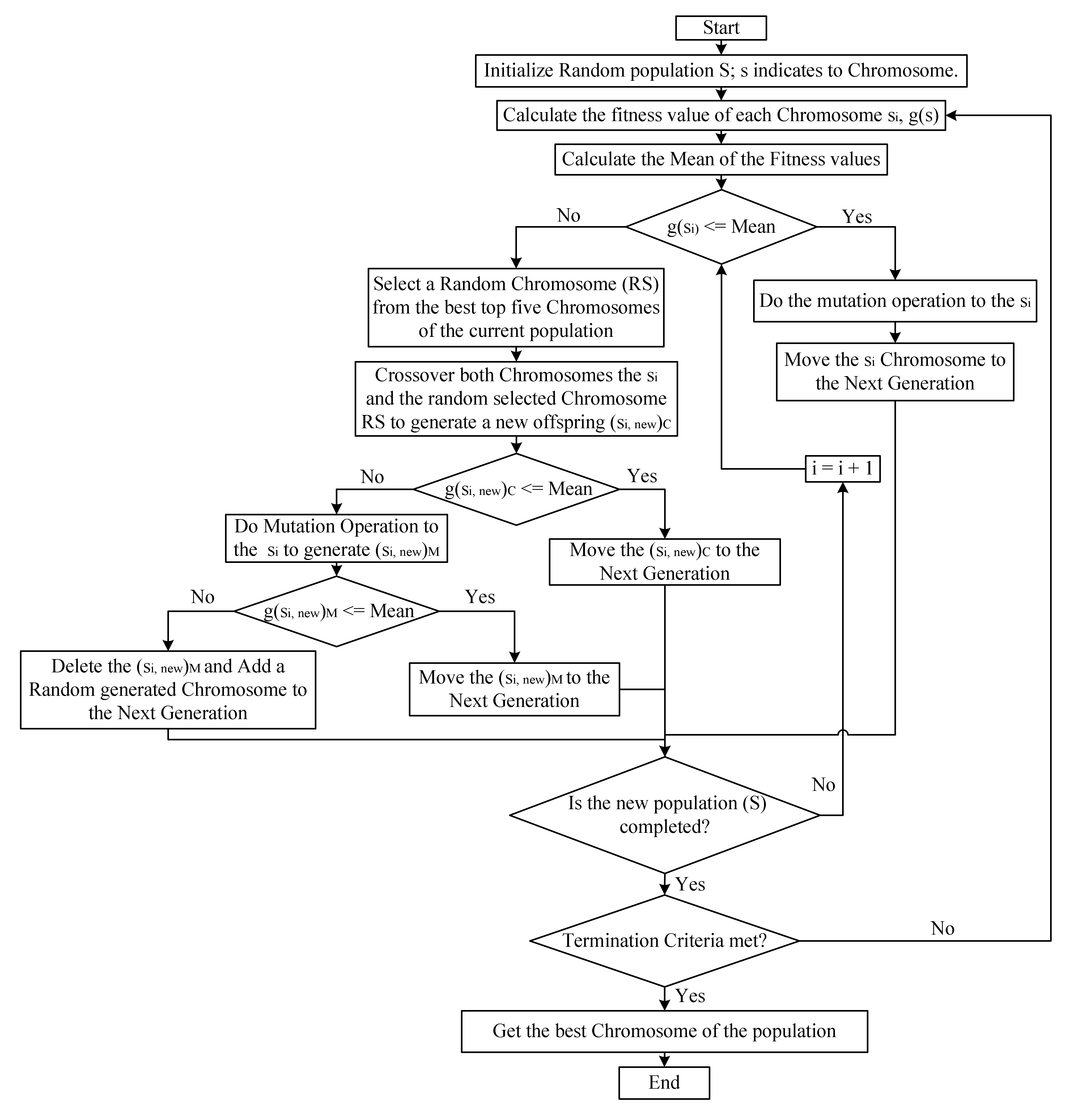
  • If g(si) is less or equal to the mean then implement the mutation operation on the si and move to the next generation. This represents the right side of the GABONST flowchart (see Figure 2), where the right side simulates the well-qualified organisms (chromosomes) to survive the current environment.
  • Otherwise, the chromosome si will get two chances to be improved, this represents the left side of the GABONST flowchart (see Figure 2), where the left side simulates the idea of giving the unqualified organisms (chromosomes) two chances to adjust their genes and be qualified to survive the current environment:
i.
The first chance is through getting married to a well-qualified organism (crossover the weak chromosome (si) with a well-qualified chromosome (RS)). If the new chromosome (si, new)C, which is obtained by crossover si and RS, qualifies to survive the current environment (g(si, new)C less or equal to the mean) then the (si, new)C move to the next generation. Otherwise, go to the second chance, step (ii).
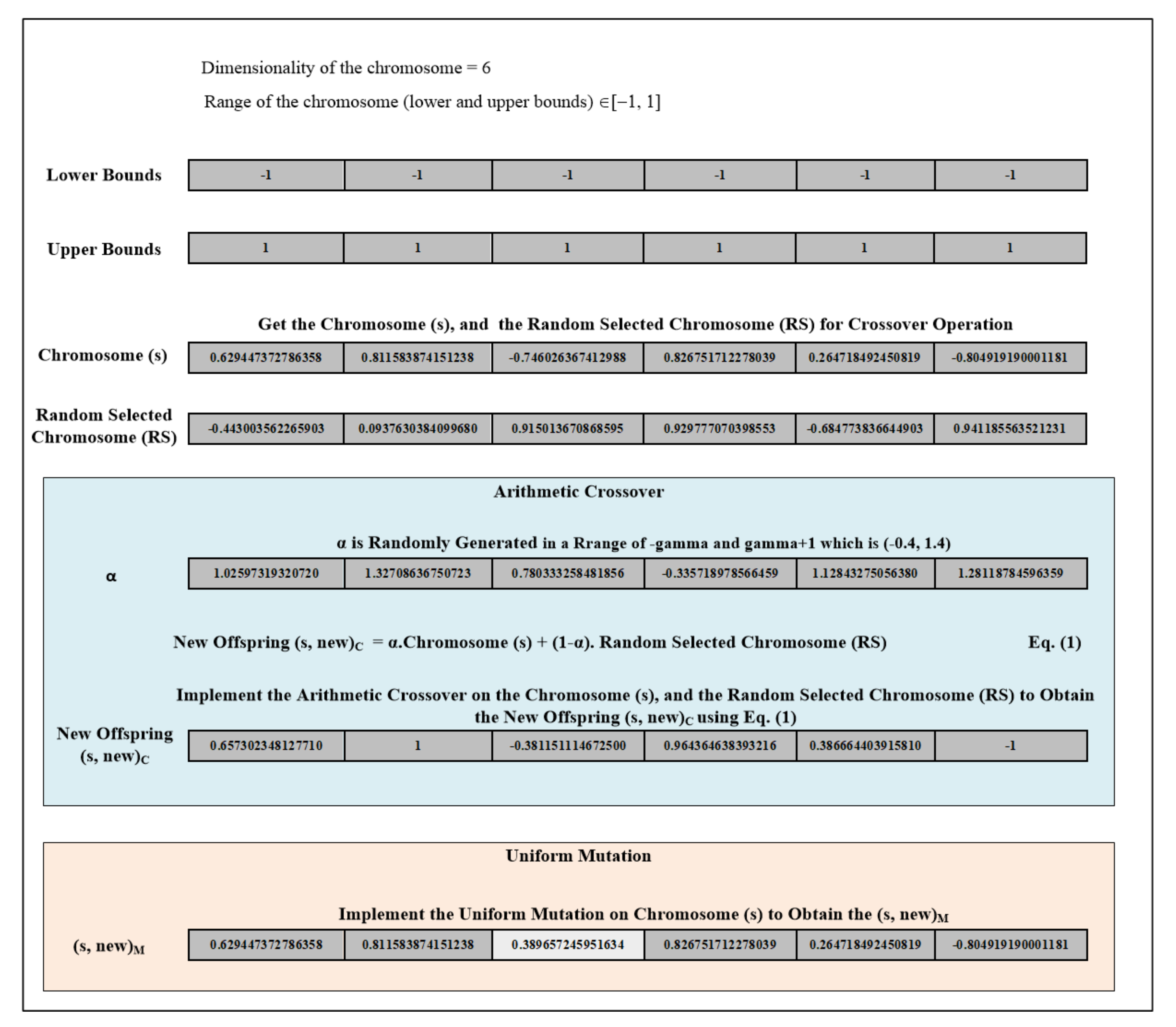
The crossover operation is subject to the boundaries (upper bounds and lower bounds). In case the value of the gene has gone beyond the max (upper bound), then we make it equal to the max (upper bound). While in the case that the value of the gene has gone lower than the min (lower bound), then we make it equal to the min (lower bound).
ii.
The second chance is through the genetic mutation (implement the mutation operation to the weak chromosome (si)). If the new chromosome (si, new)M, which is obtained by applying the mutation operation on si, qualifies to survive the current environment (g(si, new)M less or equal to the mean) then the (si, new)M move to the next generation. Otherwise, in the case that the organism (chromosome (si)) has missed both of the chances to be qualified to survive in the current environment then that organism will die (that chromosome (si) will be deleted) and a new one comes to life (add a random generated chromosome to the next generation). Figure 3 provides an example of the arithmetic crossover and uniform mutation operations that have been applied in GABONST.
Following that, the generation of the new population (S) will be obtained. S is then utilized in the ensuing iteration, whereby the whole process is run again. The process iterations will stop if there is convergence of results or if the number of iterations goes beyond the maximum threshold. The GABONST procedure is illustrated in Algorithm 1.
Algorithm 1 GABONST
  • Begin
  • Set number of population n and number of iteration NumIter.
  • Initial population. The initial population is a possible chromosome set S, which is a set of real values generated randomly, S = {s1, s2, …, sn}.
  • Evaluation. A fitness function should be defined to evaluate each chromosome in the population and can be written as fitness = g(S).
  • Calculate the Mean of the fitness values based on Equation (1).
  • Iter = 1;
  • While (Iter < NumIter)
  • i = 1;
  • While (i < n)
  • Compare the g(si) with Mean:
  • If (g(si) <= Mean)
  •  Implement mutation operation to si and move it to the next generation.
  • Else
  •  Select a random chromosome from the top five chromosomes (RS) of the current population and implement the crossover operation on both si and RS to generate (si, new)C; g(si, new)C.
  •    If (g(si, new)C <= Mean)
  •     Move the (si, new)C to the next generation.
  •    Else
  •     Implement mutation operation to si and generate (si, new)M; g(si, new)M.
  •      If (g(si, new)M <= Mean)
  •       Move the (si, new)M to the next generation.
  •      Else
  •       Delete si and add a random generated chromosome to the next generation.
  •      End if
  •    End if
  • End if
  • i = i + 1;
  • End while
  • Calculate the fitness value of each chromosome in the population g(S).
  • Calculate the Mean of the fitness values based on Equation (1).
  • Iter = Iter + 1;
  • End while
  • End

3. Results

3.1. Experimental Test One

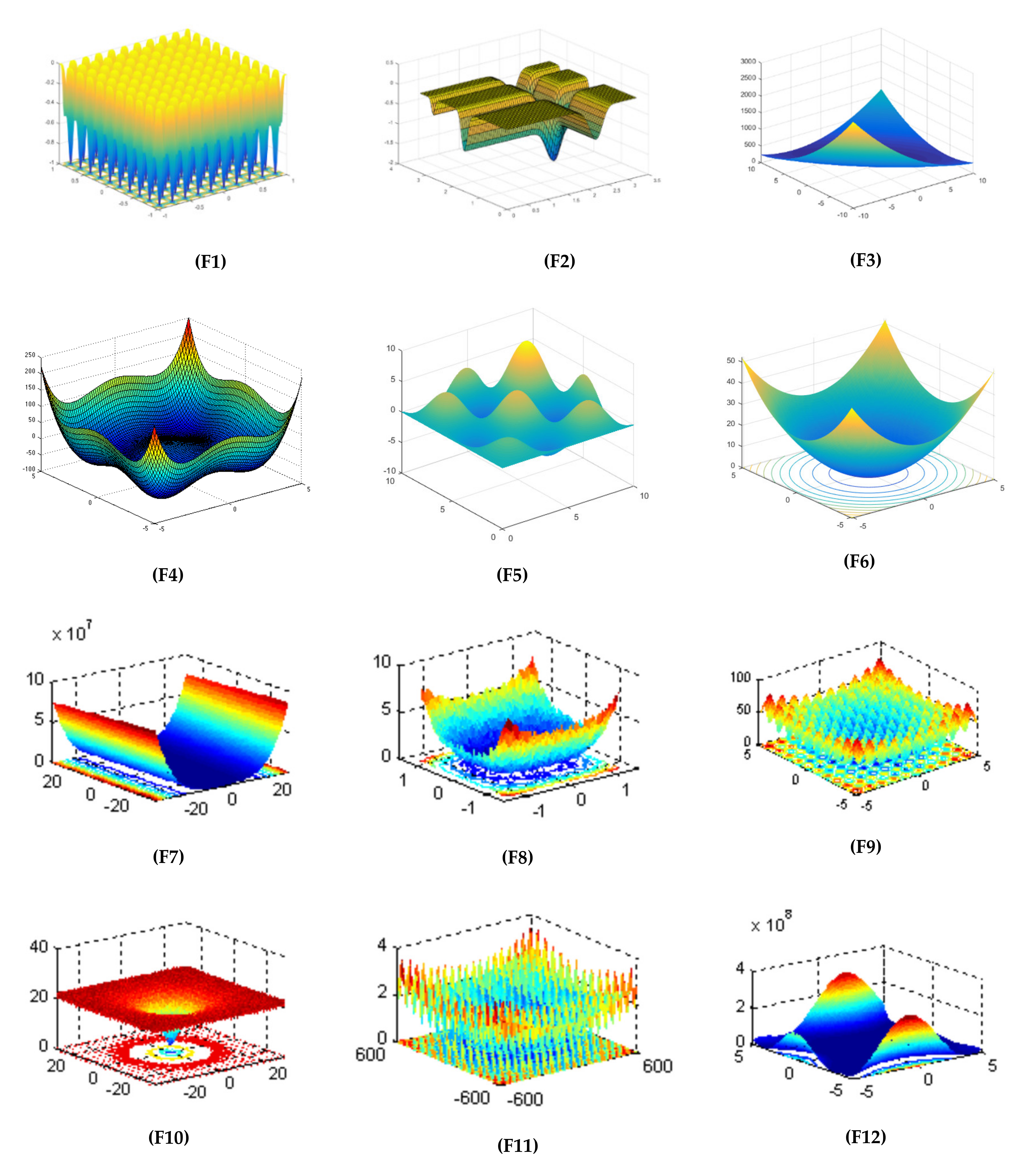
The measures for evaluating the GABONST is discussed in this section, which compares the GABONST with EATLBO, conventional GA, Bat and Bee algorithms, in terms of certain standard mathematical functions associated with the optimization surface. These algorithms underwent fifteen experiments that applied fifteen distinct objective functions, with 100 iterations and a population size of 50. The most common fifteen objective functions [51] were used to assess the performance of the optimal solution value selection in all the iterations for these algorithms. The optimal solution and dimension for each of the mathematical objective functions (F1–F15) are presented in Table 1 below. Figure 4 depicts the graphical representation of mathematical objective functions.
Table 2 presents the statistical results of the fifteen mathematical objective functions of GABONST, GA, EATLBO, Bat and Bee algorithms following the programme’s 50 runs. The most common three statistical evaluation measures were used in this study: root mean square error (RMSE), mean, and standard deviation (STD) [21,52]. The 50 results of each objective function were used to calculate the RMSE, mean, and STD. In Table 2, the values of the GABONST-RMSE and GABONST-STD are lower, which proves the effectiveness of the GABONST in terms of achieving the optimal solution. Meanwhile, the mean is close to the optimal solution (see Table 1 and Table 2), which means that the GABONST had generally attained an optimal solution in the fifteen mathematical objective functions throughout the 50 rounds, indicating that the GABONST had performed better in comparison to EATLBO, GA, Bat and Bee algorithms in terms of effectiveness and efficiency. In Table 2, the best results are shown in bold.
Based on the results in Table 2 comparing the GABONST, conventional GA, EATLBO, Bat and Bee algorithms; the GABONST have outperformed the conventional GA, EATLBO, Bat and Bee algorithms on most of the test objective functions. Except F11 and F14, where in F11 both GABONST and EATLBO have achieved the optimal solution while in F14 the conventional GA was slightly better than the GABONST (see Table 1 and Table 2). This means the GABONST is concluded to have a better performance than conventional GA, EATLBO, Bat and Bee algorithms. GABONST in this comparison is based on the idea of natural selection theory, which aims to enhance the exploration, exploitation and improve the diversity of the solutions.
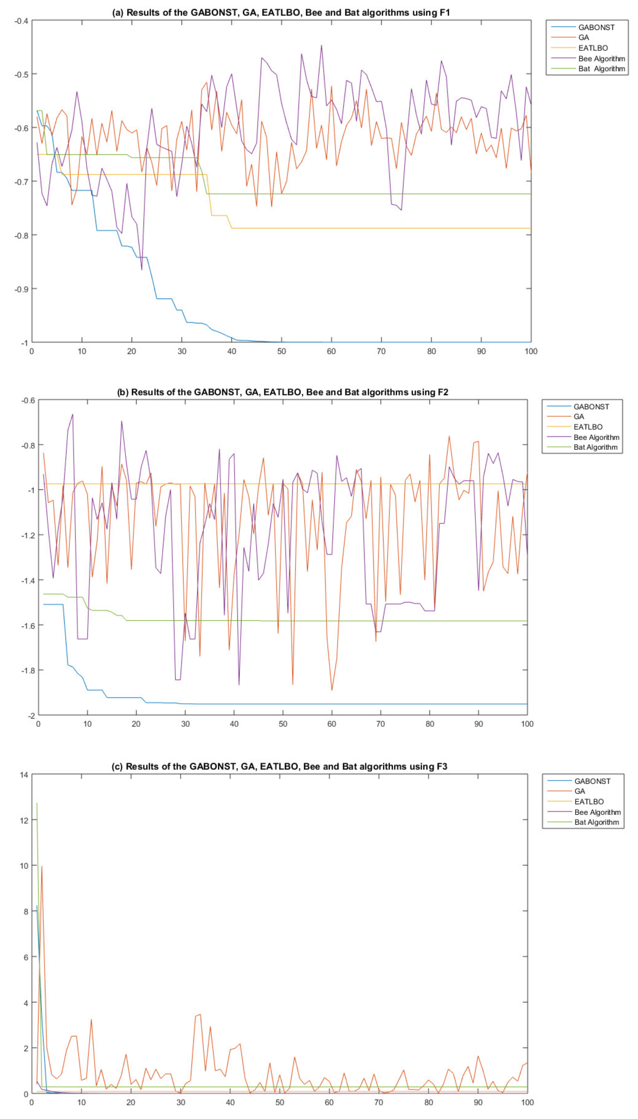
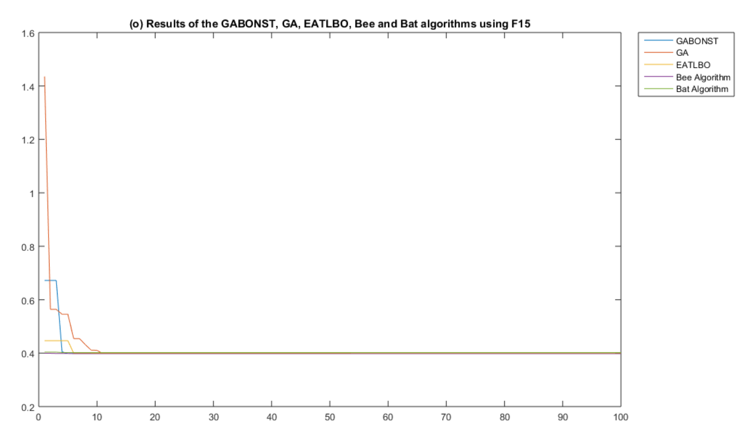
Comparatively, most of the objective functions’ experimental results clearly prove that the GABONST has faster convergence (see Figure 5). This is a result of the good exploitation and exploration offered by the idea of natural selection theory. Figure 5 depicts the comparison results that were obtained from the fifteen objective functions, which compare the GABONST against the conventional GA, EATLBO, Bat and Bee algorithms in a single run. In addition, Figure 5 proves that the reaching ability of the GABONST to the optimal solution is faster and with fewer iterations. Thus, the GABONST will be integrated into the ELM instead of the EATLBO for the purpose of adjusting the input and hidden layer weights.
The achieved results are shown in Figure 5a–o, which are based on the best solution in each iteration obtained from GABONST, GA, EATLBO, Bee and Bat algorithms using F1–F15 during a single run. The optimal solutions of the F1–F15 are provided in Table 1. The results clearly show the superiority of the GABONST over the traditional GA, EATLBO, Bee and Bat algorithms. The GABONST has achieved and reached the optimal solutions faster and with fewer iterations in comparison to the traditional GA, EATLBO, Bee and Bat algorithms.

3.2. Experimental Test Two

Additionally, this study also aims to evaluate the impact of the proposed GABONST in an application. Thus, this section will implement and evaluate the GABONST in spoken language identification (LID) by integrating the GABONST into the ELM. According to [53], ELM is a single-hidden layer feedforward neural network (SLFN), which entails the random generation of its hidden layer thresholds and input weights. Due to the fact that its output weights are computed using the least squares method, the ELM exhibits speedy training and testing functions. However, its training goal achievement and global minimum requirement are not guaranteed by the randomly generated input weights and hidden layer thresholds, indicating that both are not the best parameters for usage. Many studies have proven that the SLFN’s weight optimization as trained by the ELM using various methods is problematical. Several studies have attempted to carry out weights optimization using metaheuristic searching methods [54,55,56,57], one of which is the enhanced self-adjusting extreme learning machine (ESA-ELM) [29], which utilizes the teaching and learning phases under the framework of the enhanced ameliorated teaching learning-based optimization (EATLBO). However, the approach of optimization EATLBO is still suffering from several disadvantages such as criteria of selection and the capability of generating good fresh solutions. This could result in an incomplete optimization or a slow rate of convergence, which could not often assure achieving the optimum solution. Therefore, the aim of this study is to enhance the ELM algorithm by integrating the new proposed GABONST into the ELM instead of EATLBO and then implemented into the spoken language identification (LID). Finally, this study aims to prove the capacity of the newly offered GABONST optimization algorithm in enhancing ELM’s efficiency and effectiveness as a classifier model for LID.

3.2.1. Basic ELM

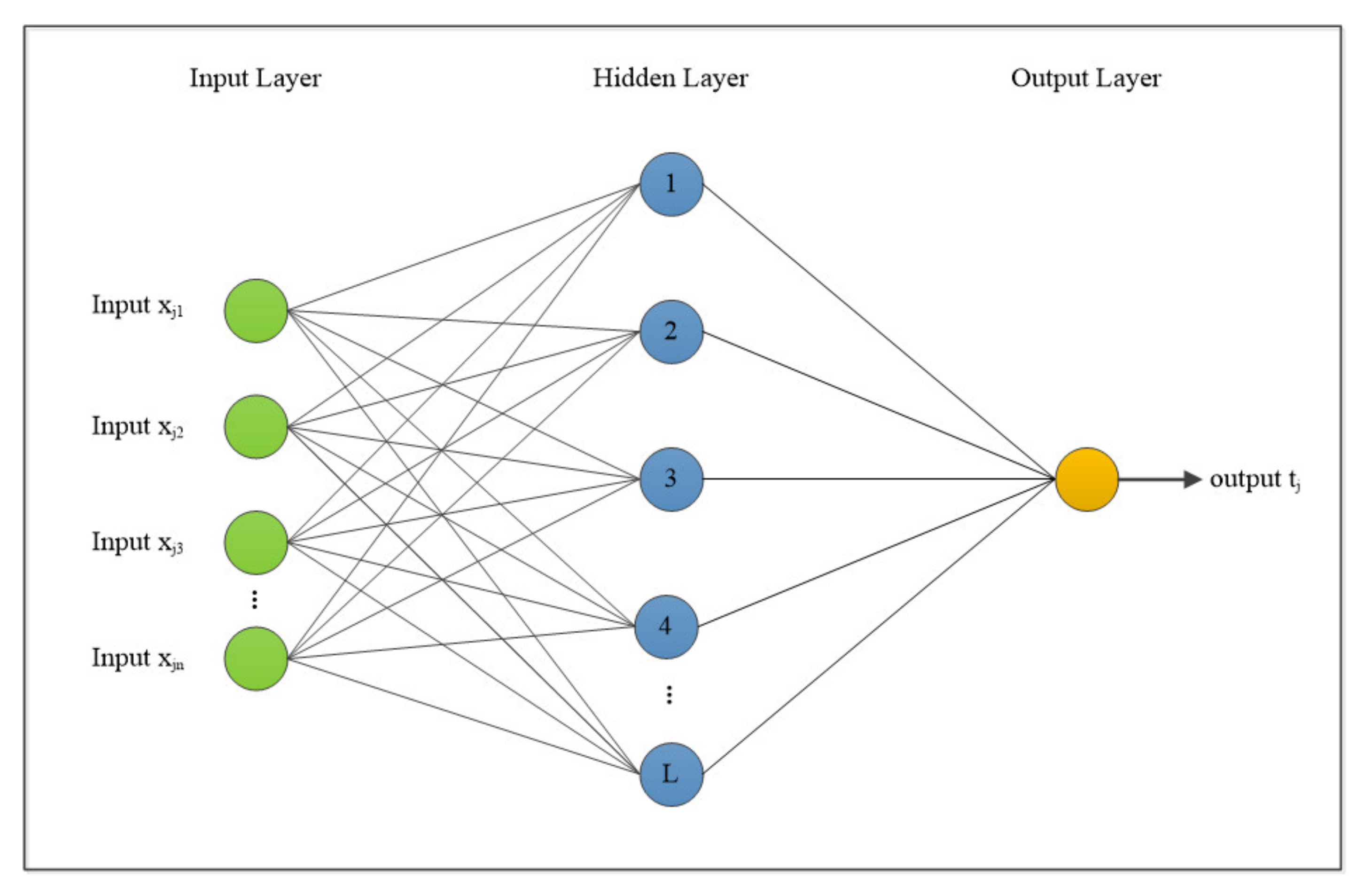
One study [53] proposed the training of SLFN by utilizing the initial ELM algorithm. The ELM’s main concepts are made up of the random bias generation and the hidden layer weights. The calculation of the output weights was done using the least squares solution as delineated by the hidden layer and the targets’ outputs. Figure 6 details the main idea of the ELM structure. The next subsection briefly explains about the ELM. Table 3 shows the ELM’s description along with its notations.
i = 1 L β i g i X j = i = 1 L β i g i W i · X j + b i = o j .
J = 1, …, N.
L = number of hidden neurons; and g(x) = activation function of the standard of SLFNs can be N samples without error.
Thus, j = 1 L | | o j t j | | = 0 , that is, β i , Wi and bi exist, such that in Equation (3) [53].
i = 1 L β i g i W i · X j + b i = t j ,   j = 1 ,   . ,   N .
The equation below is attainable by using the abovementioned equations for N [53]:
H β = T ,
where:
H W 1 W L , b 1 b L , X 1 X N = g W 1 . X 1 + b 1 g W L . X 1 + b L g W 1 . X N + b 1 g W L . X N + b L β = β 1 T β L T L m   and   T = t 1 T t N T N m
Based on [53], H entails the neural network (NN) hidden layer’s output matrix; in H, the ith column represents the ith hidden layer nodes on the input nodes. If the preferred number of hidden nodes is L ≤ N, then the activation function g can substantially be differentiated. Equation (4) then develops into a linear system. The output weights β can be systematically determined by recognizing the least squares solution as below:
β = H T
where H is the Moore–Penrose generalized inverse of H. Hence, the calculation of the output weights is based on a mathematical conversion minus a prolonged training phase. Iterative adjustments are conducted on the network parameters with several appropriate learning parameters such as learning rate and iterations.
Without an explicit approach for determining the input-hidden layer weights, the ELM is subjected to local minima, i.e., no method can ensure the usability of the trained ELM in performing the classification. This weakness can be overcome by integrating the ELM with an optimized approach in which the optimal weights are identifiable thus leading to the attainment of the ELM’s best performance. The next subsection presents the genetic algorithm based on natural selection theory-extreme learning algorithm (GABONST-ELM) after adopting the GABONST as an optimization approach into the ELM.

3.2.2. GABONST–ELM

The GABONST-ELM is based on the GABONST, which we have described in Section 2.2. GABONST-ELM uses the idea of the natural selection theory along with the GA whereby the processes of selection, crossover and mutation are used to adjust input weight values and hidden nodes bias. Table 4 summarizes the ELM and GABONST parameter values used in the experiments of this study, along with the GABONST-ELM description.
Random definitions of the input weights values and hidden nodes are carried out at the onset of the GABONST-ELM and of which were regarded as chromosomes.
Vis   C = w 11 , w 12 , w 1 n , w 21 , w 22 , w 2 n , w m 1 , w m 2 , w mn , b 1 , b m
where:
  • wij [−1, 1], is the input weight value that connect ith hidden node and jth input node
  • bi [0, 1] = ith hidden node bias
  • n = input node numbers
  • m = hidden node numbers
  • m × (n + 1) represents the chromosome’s dimension, hence requiring parameter optimizations. Therefore, the fitness function in the GABONST–ELM set is calculated utilizing Equation (6).
f C = j N | | k m β k g ( w k x j + b k ) y j | | 2 2 N
where
  • β : output weight matrix
  • yj: true value
  • N: number of training samples
The procedure of the GABONST-ELM is explained in the following steps:
Firstly, the target function fitness value is calculated for each chromosome C in the population. The fitness value f(Ci) of each C is calculated in order to evaluate C against the mean.
Secondly, the mean of the fitness values is calculated: Mean = i PS f C i PS . The mean of the fitness values is calculated in order to simulate the environment in biological theory.
Thirdly, compare each chromosome’s fitness value with the mean value. If that chromosome’s fitness value is equal to or less than the mean then the uniform mutation operation is implemented on that chromosome and moves it into the new generation. This simulates the well-qualified organisms’ (chromosomes’) survival of the current environment. If that chromosome’s fitness value greater than the mean then that chromosome will obtain two chances to be improved. This simulates the idea of giving the unqualified organisms (chromosomes) two chances to adjust their genes and become qualified to survive the current environment:
A. 
The arithmetical crossover operation is used for exchanging information between that chromosome and a randomly selected chromosome from the top five chromosomes of the current population. The new offspring will be compared to the mean:
If it is equal to or less than the mean then move the new offspring into the new generation.
If it is greater than the mean then implement step B.
B. 
The uniform mutation operation is applied to change the genes of that chromosome and generate a new chromosome. The new chromosome will be compared to the mean: if it is equal to or less than the mean then move it into the new generation. If it is greater than the mean then delete that chromosome and add a randomly generated chromosome.
Upon the generation of the new population, the subsequent iteration resumes using this new population, and the whole procedure is reiterated. This iterative process can be stopped when the number of iterations exceeds the maximum limit. The GABONST optimization results are utilized as the input weights and the hidden layer biases of ELM, computing the hidden layers’ output matrix H using the activation function g(x). Additionally, the output weights β are calculated using Equation (5) whilst the predicting ELM model is saved for testing. Figure 7 depicts the flowchart of the GABONST-ELM.

3.2.3. LID Dataset

This study has used the exact same dataset of the benchmark [29]. Eight spoken languages namely, (1) English, (2) Malay, (3) Arabic, (4) Urdu, (5) German, (6) Spanish, (7) French and (8) Persian were chosen and verified for the purpose of recognition. Audio files were recorded for each language from its respective country’s broadcasting media channel as Table 5 provides.
A total of 15 utterances were recorded for each language, with each utterance lasting 30 s. Training utilized about 67% of the total dataset, which is equal to 80 utterances, whilst testing utilized the remaining 33%, which is equal to 40 utterances [29]. The recording of the audio files was taken from the channels listed above, whereby each one of the dataset represents one language to determine the algorithm’s robustness.
The recording of the utterances was carried out using mp3 together with a dual channel. MATLAB was used as an array entailing two columns that are much alike, despite only one being used. The uttered term corresponded to one vector of the data sampled from the audio file. The length of each utterance was 30 s and each one needed to be sampled and quantified:
  • The sampling rate is 44,100 Hz, based on the Nyquist frequency the highest frequency was 22,050 Hz. The length of 30 s utterance was approximately 1,323,000 (44,100 * 30) samples.
  • Quantization: represents real-valued numbers as integers of a 16-bit range (values from −32,768 to 32,767). The following is a depiction of the utilized dataset:
    • Name and extension of the dataset: iVectors.mat;
    • Dimension of the dataset is depicted in Table 6;
      Table 6. Dataset dimension [29].
      Table 6. Dataset dimension [29].
      Total Utterance NumberTotal Class Numberi-Vector Features Dimension of One Utterance
      1208600
    • Depiction of the class is shown in Table 7;
      Table 7. Depiction of the class [29].
      Table 7. Depiction of the class [29].
      NoClass NameUtterance Number
      1Arabic15
      2English15
      3Malay15
      4French15
      5Spanish15
      6German15
      7Persian15
      8Urdu15
    • Feature depiction (as depicted in Table 8);
      Table 8. Feature depiction [29].
      Table 8. Feature depiction [29].
      NoFeatures NameFeatures Type
      1→600i-vector valuesSingle
    • The label of the class: last column (column number 601).

3.2.4. Evaluation of the Different Learning Model Parameters

This study used [59] as the basis for the evaluation where numerous measures were applied. [59] handled the classifier evaluation issue and offered effective measures to resolve it. The supervised machine learning offers several evaluation methods for the performance assessment of the learning algorithms and classifiers. Hence, measures concerning classification quality were created in this study based on a confusion matrix that records recognized examples for each class based on their correction rate. The confusion matrix is one of the most common performance measurement techniques for machine learning classification. Each row of the confusion matrix represents the instances in a predicted class, while each column represents the instances in an actual class [59].
The formulated datasets underwent several classification experiments entailing both the ESA-ELM [29] benchmark and the GABONST-ELM, with a varied amount of hidden neurones ranging from 650–900 and a 25-step increment (following the benchmark scenario [29]). Consequently, there were a total of 11 experiments for the ESA-ELM benchmark and the GABONST-ELM, with 100 iterations for each of the tests.
The ESA-ELM (benchmark) and the GABONST-ELM were hence evaluated using several measures that are based on the ground truth, i.e., utilizing the model for predicting the outcome on the evaluation dataset or held-out data, and comparing that prediction with the real outcome. The evaluation measures were also implemented in the comparison of the benchmark with the GABONST-ELM to determine the false positive, true positive, false negative, true negative, accuracy, recall, precision, G-mean and F-measure. Equations (8)–(12) [29] present the evaluation measures used in this study.
accuracy = tp + tn tp + tn + fn + fp
precision = tp tp + fp
recall = tp tp + fn
F Measure = 2 × precision × recall precision + recall
G Mean = tp p × tn n 2
where fp = false positive, tp = true positive, fn = false negative, and tn = true negative.
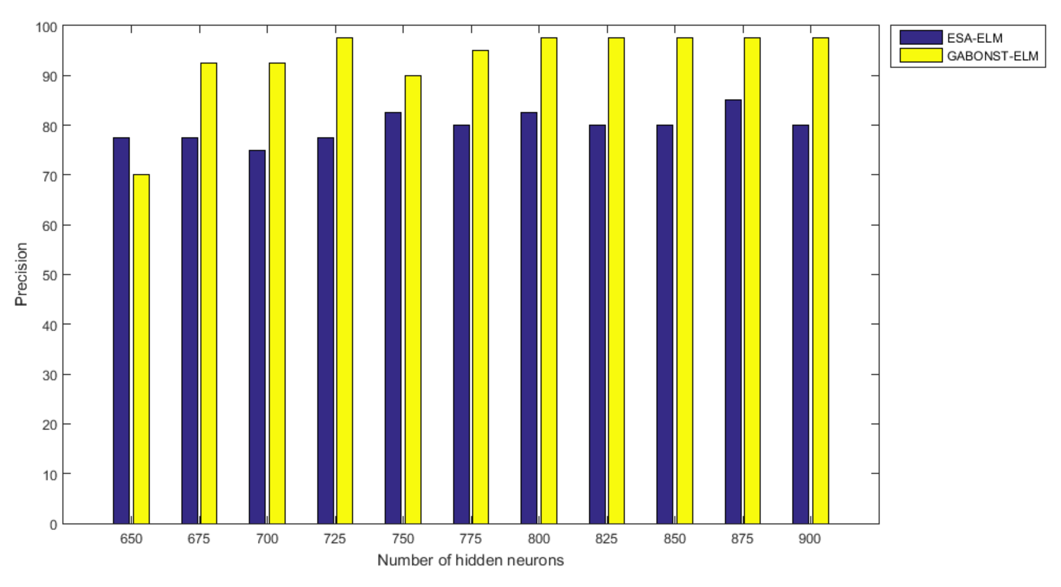
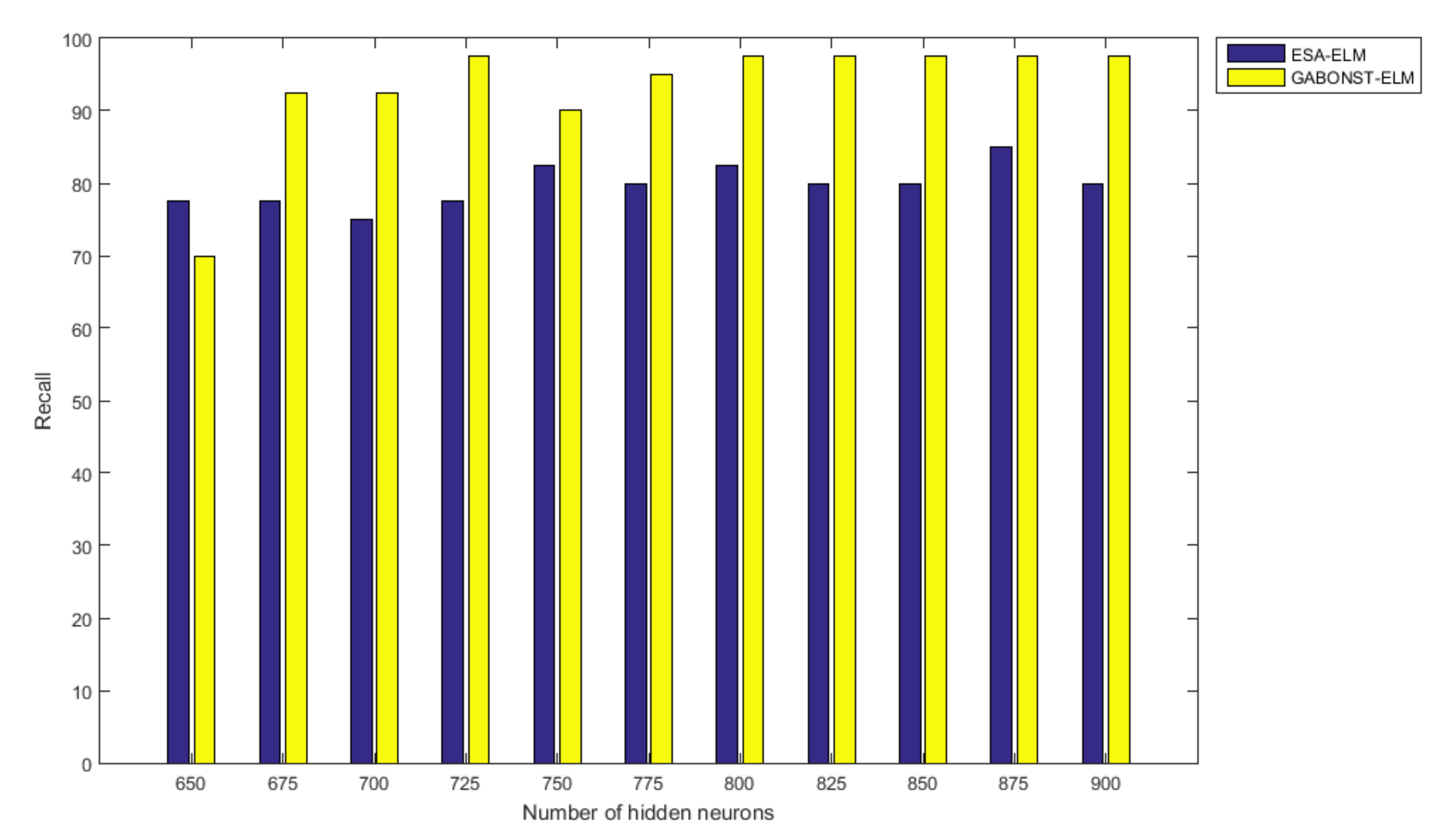
The evaluation of both approaches, ESA-ELM and GABONST-ELM, was based on the same dataset and features the extraction approach with the benchmark [29]. The results for all the experiments carried out between the ESA-ELM and the GABONST-ELM are shown in the figures below. The GABONST-ELM displayed hidden neurones accuracy in the range of 650–900, which was higher than that recorded by the ESA-ELM benchmark, indicating that the performance results of GABONST-ELM in all the iterations are more superior to that of the ESA-ELM benchmark. The comparison of results between both methods in terms of accuracy, precision, recall, F-measure and G-mean are presented in Figure 8, Figure 9, Figure 10, Figure 11 and Figure 12. The GABONST-ELM achieved the highest accuracy with 725, 800–875 neurons whilst the ESA-ELM achieved an accuracy of 875 neurons (see Figure 8). The GABONST-ELM achieved 99.38% accuracy whilst the ESA-ELM achieved a slightly lower accuracy at 96.25%. The outcomes for ESA-ELM for the other measures are precision 85.00%, recall 85.00%, G-mean 73.41%, and F-measure 85.00%. Meanwhile, GABONST-ELM recorded higher results for all the other measures i.e., recall 97.50%, precision 97.50%, F-measure 97.50% and G-mean 95.06%. The following Table 9 and Table 10 present all the results of the evaluation measures for both the ESA-ELM and GABONST-ELM:
Moreover, other experiments were conducted utilizing the i-vector features and the neural network (NN) classifier. “Adam” optimizer and rectified linear unit (ReLU) activation function have been used in the NN. The NN was implemented in LID based on the exact same benchmark’s dataset (see Section 3.2.3) with variation of the hidden neuron numbers in the range of 650–900 with an increment step of 25. Table 11 provides all results of the NN during all experiments.
Additionally, several experiments were performed based on the benchmark’s dataset (see Section 3.2.3) for the basic ELM and fast learning network (FLN) with varying numbers of hidden neurons within the range of 650–900 with an increment of 25. Table 12 and Table 13 provide the experiment results of the basic ELM and FLN. The highest performance of the basic ELM was achieved with 875 neurons, and the achieved accuracy was 89.38%. The results of other evaluation measures were 57.50%, 57.50%, 57.50% and 40.53% for F-measure, precision, recall, and G-mean, respectively. The highest performance of the FLN was achieved with 725 neurons, and the achieved accuracy was 92.50%. The results of other evaluation measures were 70.00%, 70.00%, 70.00%, and 53.44% for F-measure, precision, recall, and G-mean, respectively.
In addition, several experiments were conducted based on the benchmark’s dataset (see Section 3.2.3) for the genetic algorithm-extreme learning machine (GA-ELM), bat-extreme learning machine (Bat-ELM), and bee-extreme learning machine (Bee-ELM) with varying numbers of hidden neurons within the range of 650–900 and an increment of 25. Table 14, Table 15 and Table 16 provide the experiment results of the GA-ELM, Bat-ELM, and Bee-ELM.
As the results show in Table 9, Table 10, Table 11, Table 12, Table 13, Table 14, Table 15 and Table 16, the performance of GABONST-ELM outperformed the basic ELM, FLN, NN, GA-ELM, Bat-ELM, Bee-ELM and the benchmark ESA-ELM in all experiments. This finding confirms that generating suitable biases and weights for the ELM with single hidden layer reduces classification errors. Avoiding unsuitable biases and weights prevents the ELM from becoming stuck in the local maxima of biases and weights. Therefore, the performance of GABONST-ELM is very impressive, with an accuracy of 99.38%.

4. Conclusions

In this study, we proposed the new GABONST based on the existing genetic algorithm (GA) for the optimization problem. GABONST has the same concept as the conventional GA, which imitated the biological structure of the natural world based on Darwin’s principles that are made up of three operations, i.e., selection, crossover, and mutation. The GABONST enhanced the conventional GA based on the idea of natural selection theory. It is worth mentioning that all the experiments have been implemented in MATLAB programming language. Based on the algorithm implementation and its results in fifteen different standard test objective functions, the algorithm has shown to be more effective than the conventional GA. This algorithm is primarily advantageous due to its focus on the search space’s better area, which resulted from a good exploration–exploitation balance. The good exploration results from the idea of (i) giving the chromosomes that do not satisfy the mean two chances to be improved via the crossover and mutation operations. (ii) By deleting the chromosomes that obtained the two chances and still do not satisfy the mean and adding a randomly generated chromosome. Whilst the good exploitation results from using the idea of the mean that intensifies the search space in the best region. Such an advantage allows for the algorithm’s achievement of better convergence. The GABONST is proven to have a better performance than the conventional GA and EATLBO based on the statistical analysis. Additionally, the GABONST-ELM outperformed the ESA-ELM in LID through adopting the GABONST into the ELM instead of EATLBO. Following this study, the plan is to investigate new alternative selection criteria and integrate them into the concept of choosing a chromosome for the crossover operation instead of random selection criteria and apply it on several possible applications.

Author Contributions

Conceptualization, methodology, writing—original draft, software, writing—review and editing: M.A.A.; supervision, funding acquisition, project administration: S.T.; supervision: M.A.; writing—review and editing, investigation: F.A.-D. All authors have read and agreed to the published version of the manuscript.

Funding

This project was under the funding of the Malaysian government with the research code: GUP-2020-063.

Conflicts of Interest

The authors declare no conflict of interest.

References

  1. Alzaqebah, M.; Abdullah, S. An adaptive artificial bee colony and late-acceptance hill-climbing algorithm for examination timetabling. J. Sched. 2013, 17, 249–262. [Google Scholar] [CrossRef]
  2. Alzaqebah, M.; Abdullah, S. Hybrid bee colony optimization for examination timetabling problems. Comput. Oper. Res. 2015, 54, 142–154. [Google Scholar] [CrossRef]
  3. Aziz, R.A.; Ayob, M.; Othman, Z.; Ahmad, Z.; Sabar, N.R. An adaptive guided variable neighborhood search based on honey-bee mating optimization algorithm for the course timetabling problem. Soft Comput. 2016, 21, 6755–6765. [Google Scholar] [CrossRef]
  4. Sabar, N.R.; Ayob, M.; Kendall, G.; Qu, R. A honey-bee mating optimization algorithm for educational timetabling problems. Eur. J. Oper. Res. 2012, 216, 533–543. [Google Scholar] [CrossRef] [Green Version]
  5. Jaddi, N.S.; Abdullah, S.; Hamdan, A.R. Multi-population cooperative bat algorithm-based optimization of artificial neural network model. Inf. Sci. 2015, 294, 628–644. [Google Scholar] [CrossRef]
  6. Jaddi, N.S.; Abdullah, S.; Hamdan, A.R. A solution representation of genetic algorithm for neural network weights and structure. Inf. Process. Lett. 2016, 116, 22–25. [Google Scholar] [CrossRef]
  7. Serapião, A.B.; Corrêa, G.S.; Gonçalves, F.B.; Carvalho, V.O. Combining K-Means and K-Harmonic with Fish School Search Algorithm for data clustering task on graphics processing units. Appl. Soft Comput. 2016, 41, 290–304. [Google Scholar] [CrossRef] [Green Version]
  8. Hassanien, A.E.; Moftah, H.M.; Azar, A.T.; Shoman, M. MRI breast cancer diagnosis hybrid approach using adaptive ant-based segmentation and multilayer perceptron neural networks classifier. Appl. Soft Comput. 2014, 14, 62–71. [Google Scholar] [CrossRef]
  9. Krishna, P.V. Honey bee behavior inspired load balancing of tasks in cloud computing environments. Appl. Soft Comput. 2013, 13, 2292–2303. [Google Scholar]
  10. Albadr, M.A.A.; Tiun, S. Spoken Language Identification Based on Particle Swarm Optimisation–Extreme Learning Machine Approach. Circuits Syst. Signal. Process. 2020, 1–27. [Google Scholar] [CrossRef]
  11. Albadr, M.A.A.; Tiun, S.; Ayob, M.; Al-Dhief, F.T. Spoken language identification based on optimised genetic algorithm–extreme learning machine approach. Int. J. Speech Technol. 2019, 22, 711–727. [Google Scholar] [CrossRef]
  12. Yassen, E.T.; Ayob, M.; Nazri, M.Z.A.; Sabar, N.R. A Hybrid Meta-Heuristic Algorithm for Vehicle Routing Problem with Time Windows. Int. J. Artif. Intell. Tools 2015, 24, 1550021. [Google Scholar] [CrossRef]
  13. Yassen, E.T.; Ayob, M.; Nazri, A.; Zakree, M. The Effect of Hybridizing Local Search Algorithms with Harmony Search for the Vehicle Routing Problem with Time Windows. J. Theor. Appl. Inf. Technol. 2015, 73, 43–58. [Google Scholar]
  14. Yassen, E.T.; Ayob, M.; Nazri, M.Z.A.; Sabar, N.R. Meta-harmony search algorithm for the vehicle routing problem with time windows. Inf. Sci. 2015, 325, 140–158. [Google Scholar] [CrossRef]
  15. Agarwal, P.; Mehta, S. Nature-Inspired Algorithms: State-of-Art, Problems and Prospects. Int. J. Comput. Appl. 2014, 100, 14–21. [Google Scholar] [CrossRef]
  16. Jaddi, N.S.; Abdullah, S. Optimization of neural network using kidney-inspired algorithm with control of filtration rate and chaotic map for real-world rainfall forecasting. Eng. Appl. Artif. Intell. 2018, 67, 246–259. [Google Scholar] [CrossRef]
  17. Poli, R.; Kennedy, J.; Blackwell, T. Particle swarm optimization. Swarm Intell. 2007, 1, 33–57. [Google Scholar] [CrossRef]
  18. Holland, J.H. Adaptation in Natural and Artificial Systems: An Introductory Analysis with Applications to Biology, Control, and Artificial Intelligence; MIT press: Cambridge, MA, USA, 1992. [Google Scholar]
  19. Yang, X.-S. A new metaheuristic bat-inspired algorithm. In Nature Inspired Cooperative Strategies for Optimization (NICSO 2010); Springer: Berlin/Heidelberg, Germany, 2010; pp. 65–74. [Google Scholar]
  20. Geem, Z.W.; Kim, J.H.; Loganathan, G. A New Heuristic Optimization Algorithm: Harmony Search. Simulation 2001, 76, 60–68. [Google Scholar] [CrossRef]
  21. Jaddi, N.S.; Alvankarian, J.; Abdullah, S. Kidney-inspired algorithm for optimization problems. Commun. Nonlinear Sci. Numer. Simul. 2017, 42, 358–369. [Google Scholar] [CrossRef]
  22. Goldberg, D.E.; Holland, J.H. Genetic algorithms and machine learning. Mach. Learn. 1988, 3, 95–99. [Google Scholar] [CrossRef]
  23. Holland, J.H. Genetic algorithms. Sci. Am. 2012, 7, 1482. [Google Scholar] [CrossRef]
  24. Mirjalili, S. Genetic algorithm. In Evolutionary Algorithms and Neural Networks; Springer: New York, NY, USA, 2019; pp. 43–55. [Google Scholar] [CrossRef] [Green Version]
  25. Contreras-Bolton, C.; Parada, V. Automatic Combination of Operators in a Genetic Algorithm to Solve the Traveling Salesman Problem. PLoS ONE 2015, 10, e0137724. [Google Scholar] [CrossRef] [PubMed] [Green Version]
  26. Anam, S. Parameters Estimation of Enzymatic Reaction Model for Biodiesel Synthesis by Using Real Coded Genetic Algorithm with Some Crossover Operations; IOP Publishing: Bristol, UK, 2019; Volume 546, p. 052006. [Google Scholar]
  27. Malik, A. A Study of Genetic Algorithm and Crossover Techniques. Int. J. Comput. Sci. Mob. Comput. 2019, 8, 335–344. [Google Scholar]
  28. Mankad, K.B. A Genetic Fuzzy Approach to Measure Multiple Intelligence; Sardar Patel University: Gujarat, India, 2013. [Google Scholar]
  29. Albadr, M.A.A.; Tiun, S.; Al-Dhief, F.T.; Sammour, M.A.M. Spoken language identification based on the enhanced self-adjusting extreme learning machine approach. PLoS ONE 2018, 13, e0194770. [Google Scholar] [CrossRef] [Green Version]
  30. Holland, J.H. Adaption in Natural and Artificial Systems. An Introductory Analysis with Application to Biology, Control and Artificial Intelligence, 1st ed.; The University of Michigan: Ann Arbor, MI, USA, 1975. [Google Scholar]
  31. Bi, C. Deterministic local alignment methods improved by a simple genetic algorithm. Neurocomputing 2010, 73, 2394–2406. [Google Scholar] [CrossRef]
  32. Mohamed, M.H. Rules extraction from constructively trained neural networks based on genetic algorithms. Neurocomputing 2011, 74, 3180–3192. [Google Scholar] [CrossRef]
  33. Höschel, K.; Lakshminarayanan, V. Genetic algorithms for lens design: A review. J. Opt. 2018, 48, 134–144. [Google Scholar] [CrossRef] [Green Version]
  34. Michalewicz, Z. Genetic Algorithms + Data Structures = Evolution Programs. Math. Intell. 1996, 18, 71. [Google Scholar] [CrossRef]
  35. Yu, F.; Fu, X.; Li, H.; Dong, G. Improved Roulette Wheel Selection-Based Genetic Algorithm for TSP. In Proceedings of the 2016 International Conference on Network and Information Systems for Computers (ICNISC), Wuhan, China, 15–17 April 2016; pp. 151–154. [Google Scholar]
  36. Zhi, H.; Liu, S. Face recognition based on genetic algorithm. J. Vis. Commun. Image Represent. 2019, 58, 495–502. [Google Scholar] [CrossRef]
  37. Zhang, H.; Xie, J.; Ge, J.; Zhang, Z.; Zong, B. A hybrid adaptively genetic algorithm for task scheduling problem in the phased array radar. Eur. J. Oper. Res. 2019, 272, 868–878. [Google Scholar] [CrossRef]
  38. Wong, K.-W.; Yap, W.-S.; Wong, D.C.-K.; Phan, R.C.-W.; Goi, B.-M. Cryptanalysis of genetic algorithm-based encryption scheme. Multimedia Tools Appl. 2020, 79, 25259–25276. [Google Scholar] [CrossRef]
  39. Ahmed, R.; Zayed, T.; Nasiri, F. A Hybrid Genetic Algorithm-Based Fuzzy Markovian Model for the Deterioration Modeling of Healthcare Facilities. Algorithms 2020, 13, 210. [Google Scholar] [CrossRef]
  40. Kar, S.; Kabir, M.M.J. Comparative Analysis of Mining Fuzzy Association Rule using Genetic Algorithm. In Proceedings of the 2019 International Conference on Electrical, Computer and Communication Engineering (ECCE), Cox’sBazar, Bangladesh, 7–9 February 2019; pp. 1–5. [Google Scholar]
  41. Tan, X.; Wu, J.; Mao, T.; Tan, Y. Multi-attribute intelligent decision-making method based on triangular fuzzy number hesitant intuitionistic fuzzy sets. Syst. Eng. Electron. 2017, 39, 829–836. [Google Scholar]
  42. Li, X.; Wang, Z.; Sun, Y.; Zhou, S.; Xu, Y.; Tan, G. Genetic algorithm-based content distribution strategy for F- RAN architectures. ETRI J. 2019, 41, 348–357. [Google Scholar] [CrossRef]
  43. Serbanescu, M.-S. Genetic algorithm/extreme learning machine paradigm for cancer detection. Ann. Univ. Craiova Math. Comput. Sci. Ser. 2019, 46, 372–380. [Google Scholar]
  44. Choudhary, A.; Kumar, M.; Gupta, M.K.; Unune, D.K.; Mia, M. Mathematical modeling and intelligent optimization of submerged arc welding process parameters using hybrid PSO-GA evolutionary algorithms. Neural Comput. Appl. 2019, 1–14. [Google Scholar] [CrossRef] [Green Version]
  45. Jamali, B.; Rasekh, M.; Jamadi, F.; Gandomkar, R.; Makiabadi, F. Using PSO-GA algorithm for training artificial neural network to forecast solar space heating system parameters. Appl. Therm. Eng. 2019, 147, 647–660. [Google Scholar] [CrossRef]
  46. Lipare, A.; Edla, D.R.; Cheruku, R.; Tripathi, D. GWO-GA Based Load Balanced and Energy Efficient Clustering Approach for WSN. In Smart Trends in Computing and Communications; Springer: Singapore, 2020; pp. 287–295. [Google Scholar] [CrossRef]
  47. Beg, A.H.; Islam, Z. Novel crossover and mutation operation in genetic algorithm for clustering. In Proceedings of the 2016 IEEE Congress on Evolutionary Computation (CEC), Vancouver, BC, Canada, 24–29 July 2016; pp. 2114–2121. [Google Scholar] [CrossRef]
  48. Kora, P.; Yadlapalli, P. Crossover Operators in Genetic Algorithms: A Review. Int. J. Comput. Appl. 2017, 162, 34–36. [Google Scholar] [CrossRef]
  49. Darwin, C.; Wallace, A.R. Evolution by Natural Selection; Cambridge University Press: Cambridge, UK, 1958. [Google Scholar]
  50. Livezey, R.L.; Darwin, C. On the Origin of Species by Means of Natural Selection. Am. Midl. Nat. 1953, 49, 937. [Google Scholar] [CrossRef] [Green Version]
  51. Jamil, M.; Yang, X.S. A literature survey of benchmark functions for global optimisation problems. Int. J. Math. Model. Numer. Optim. 2013, 4, 150–194. [Google Scholar] [CrossRef] [Green Version]
  52. Jain, M.; Singh, V.; Rani, A. A novel nature-inspired algorithm for optimization: Squirrel search algorithm. Swarm Evol. Comput. 2019, 44, 148–175. [Google Scholar] [CrossRef]
  53. Huang, G.-B.; Zhu, Q.-Y.; Siew, C.-K. Extreme learning machine: Theory and applications. Neurocomputing 2006, 70, 489–501. [Google Scholar] [CrossRef]
  54. Alexander, V.; Annamalai, P. An Elitist Genetic Algorithm Based Extreme Learning Machine. Softw. Eng. Intell. Syst. 2015, 301–309. [Google Scholar] [CrossRef]
  55. Nayak, P.K.; Mishra, S.; Dash, P.K.; Bisoi, R. Comparison of modified teaching–learning-based optimization and extreme learning machine for classification of multiple power signal disturbances. Neural Comput. Appl. 2015, 27, 2107–2122. [Google Scholar] [CrossRef]
  56. Niu, P.; Ma, Y.; Li, M.; Yan, S.; Li, G. A Kind of Parameters Self-adjusting Extreme Learning Machine. Neural Process. Lett. 2016, 44, 813–830. [Google Scholar] [CrossRef]
  57. Yang, Z.; Zhang, T.; Zhang, D. A novel algorithm with differential evolution and coral reef optimization for extreme learning machine training. Cogn. Neurodyn. 2015, 10, 73–83. [Google Scholar] [CrossRef] [Green Version]
  58. Albadra, M.A.A.; Tiuna, S. Extreme learning machine: A review. Int. J. Appl. Eng. Res. 2017, 12, 4610–4623. [Google Scholar]
  59. Sokolova, M.; Japkowicz, N.; Szpakowicz, S. Beyond Accuracy, F-Score and ROC: A Family of Discriminant Measures for Performance Evaluation; Springer: Berlin/Heidelberg, Germany, 2006; pp. 1015–1021. [Google Scholar]
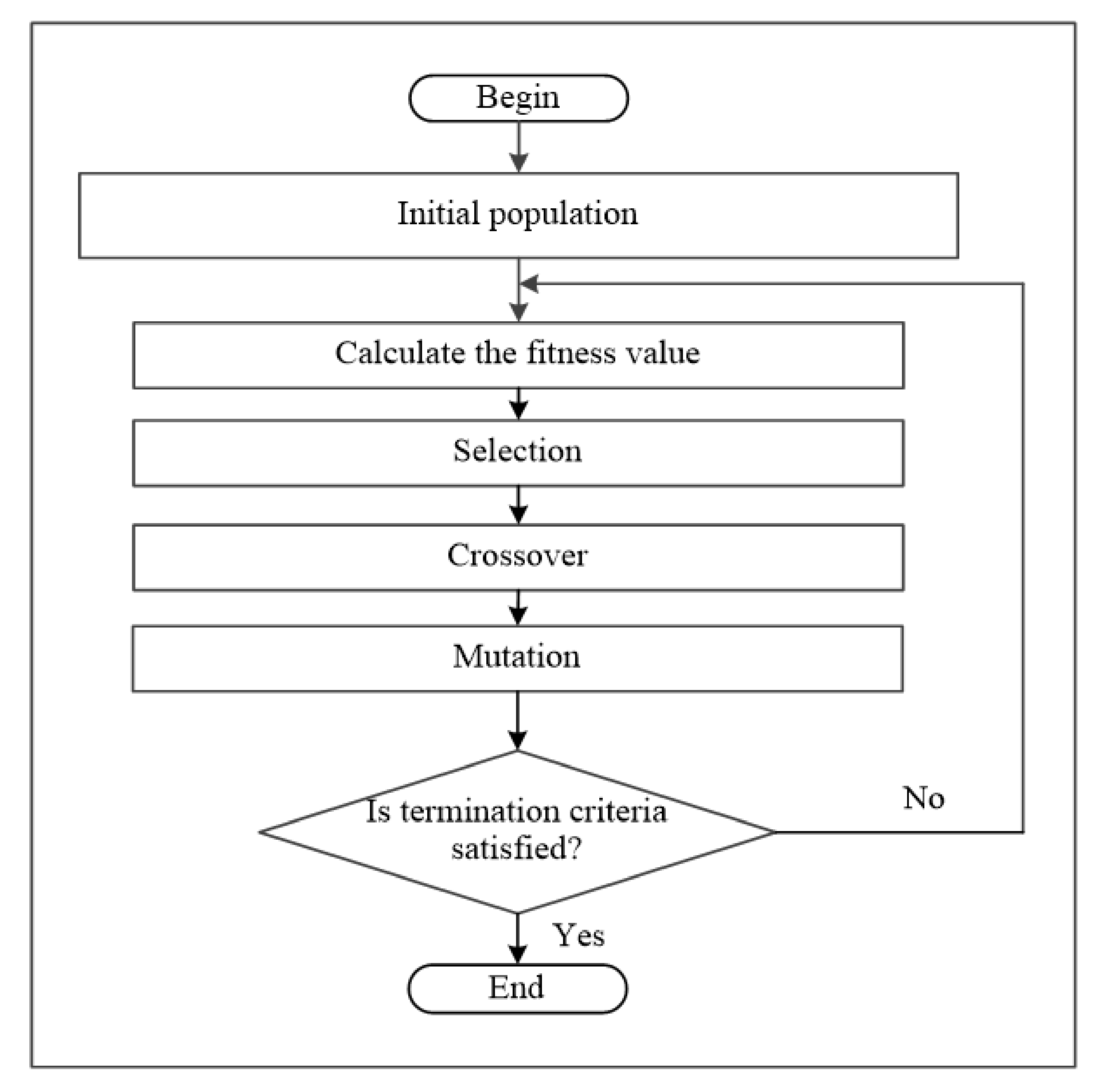
Figure 1. Flowchart of the standard genetic algorithm (GA) [33].
Symmetry 12 01758 g001
Figure 2. Flowchart of the genetic algorithm based on natural selection theory (GABONST).
Symmetry 12 01758 g002
Figure 3. Diagram of the arithmetic crossover and uniform mutation operations example.
Symmetry 12 01758 g003
Figure 4. Graphical representation of mathematical objective functions (mathematical objective functions F1F15 in Table 1).
Symmetry 12 01758 g004aSymmetry 12 01758 g004b
Figure 5. The comparison results of GABONST, GA, EATLBO, Bee and Bat algorithms using the fifteen objective functions (F1F15).
Symmetry 12 01758 g005aSymmetry 12 01758 g005bSymmetry 12 01758 g005cSymmetry 12 01758 g005dSymmetry 12 01758 g005e
Figure 6. Diagram of the ELM [58].
Symmetry 12 01758 g006
Figure 7. Flowchart of the genetic algorithm based on natural selection theory-extreme learning algorithm (GABONST-ELM).
Symmetry 12 01758 g007
Figure 8. Accuracy results of the GABONST-ELM and enhanced self-adjusting extreme learning machine (ESA-ELM).
Symmetry 12 01758 g008
Figure 9. Precision results of the GABONST-ELM and ESA-ELM.
Symmetry 12 01758 g009
Figure 10. Recall results of the GABONST-ELM and ESA-ELM.
Symmetry 12 01758 g010
Figure 11. F-measure results of the GABONST-ELM and ESA-ELM.
Symmetry 12 01758 g011
Figure 12. G-mean results of the GABONST-ELM and ESA-LEM.
Symmetry 12 01758 g012
Table 1. Details of the utilized mathematical objective functions.
Objective FunctionDimRangeOptimal Solution
f 1 x = 1 d i = 1 d sin 6 5 π x i 10[−1, 1]−1
f 2 x = i = 1 d sin x i   sin 2 m ix i 2 π 2[0, π]−1.8013
f 3 x = x 1 + 2 x 2 7 2 + 2 x 1 + x 2 5 2 2[−10, 10]0
f 4 x = 1 2 i = 1 d x i 4 16 x i 2 + 5 x i 10[−5, 5]−391.6599
f 5 x = i = 1 d x i sin x i 2[0, 10]−6.1295
f 6 x = i = 1 n x i 2 256[−5.12, 5.12]0
f 7 x = i = 1 n 1 100 x i + 1 x i 2 2 + x i 1 2 30[−30, 30]0
f 8 x = i = 1 n ix i 4 + random 0 , 1 30[−1.28, 1.28]0
f 9 x = i = 1 n x i 2 10 cos 2 π x i + 10 30[−5.12, 5.12]0
f 10 x = 20 exp 0.2 1 n i = 1 n x i 2 exp 1 n i = 1 n cos ( 2 π x i ) + 20 + e 128[−32.768, 32.768]0
f 11 x = 1 4000 i = 1 n x i 2 i = 1 n cos x i i + 1 30[−600, 600]0
f 12 x = [ 1 + x 1 + x 2 + 1 2 ( 19 14 x 1 + 3 x 1 2 14 x 2 + 6 x 1 x 2 + 3 x 2 2 ) × 30 + 2 x 1 3 x 2 2 × 18 32 x 1 + 12 x 1 2 + 48 x 2 36 x 1 x 2 + 27 x 2 2 ] 2[−2, 2]3
f 13 x = i = 1 11 a i x 1 b i 2 + b i x 2 b i 2 + b i x 3 + x 4 2 4[−5, 5]0.00030
f 14 x = 4 x 1 2 2.1 x 1 4 + 1 3 x 1 6 + x 1 x 2 4 x 2 2 + 4 x 2 4 2[−5, 5]−1.0316
f 15 x = x 2 5.1 4 π 2 x 1 2 + 5 π x 1 6 2 + 10 1 1 8 π cos x 1 + 10 2[−5, 5]0.398
Table 2. Statistical results of the mathematical objective functions for the optimization approaches (GABONST, GA, enhanced ameliorated teaching learning-based optimization (EATLBO), Bat and Bee)).
F1F2F3F4F5
GA–RMSE0.4082660.660050.45717269.844262.734866
GABONST–RMSE0.0089120.1498015.502010
EATLBO–RMSE0.2413620.8039740.379706148.61350.715572
Bat-RMSE0.38200.40335.7316153.32580.2902
Bee-RMSE1.00000.56939.2615 × 10−10186.72170.2444
GA–Mean−0.60383−1.2071718.4889−326.997−3.7482
GABONST–Mean−0.99688−1.95110−380.897−6.1295
EATLBO–Mean−0.77554−0.997330.27178−245.971−5.67757
Bat-Mean−0.6215−1.58893.3044−240.5929−5.9602
Bee-Mean−9.4481 × 10⁻¹¹−1.30246.1739 × 10−10−207.6444−6.0014
GA–STD0.0996540.2904610.27156226.661881.358616
GABONST–STD0.0084342.24299 × 10−15011.267514.48598 × 10−15
EATLBO–STD0.0896370.002570.26785629.624790.56043
Bat-STD0.05260.34634.730726.48760.2381
Bee-STD3.1940 × 10−110.27696.9736 × 10−1031.99600.2103
F6F7F8F9F10
GA–RMSE115.03088.1381 × 1030.161242.711610.9405
GABONST–RMSE002.2336 × 10−400
EATLBO–RMSE4.4872 × 10−5628.94952.7609 × 10−4205.08042.8037
Bat-RMSE1.2039 × 1039.0087 × 10774.3799364.557120.1364
Bee-RMSE1.7538 × 1032.3143 × 10714.6593141.433619.6219
GA–Mean113.93906.7387 × 1030.146441.674210.9243
GABONST–Mean001.5895 × 10−400
EATLBO–Mean3.3624 × 10−5628.94952.0063 × 10−4202.51952.6162
Bat-Mean1.1761 × 1038.1520 × 10767.4795362.386620.1321
Bee-Mean1.7533 × 1032.1898 × 10714.3940140.496019.6218
GA–STD15.97104.6090 × 1030.06829.451639.3751
GABONST–STD001.5852 × 10−400
EATLBO–STD3.0016 × 10−560.01751.9160 × 10−432.63621.0182
Bat-STD259.86003.8731 × 10731.604740.12460.4206
Bee-STD39.37517.5653 × 1062.804916.42410.0496
F11F12F13F14F15
GA–RMSE2.23426.4588 × 10−60.00182.8284 × 10−51.1264 × 10⁻⁴
GABONST–RMSE07.6591 × 10−141.4195 × 10−42.8453 × 10−51.1264 × 10⁻⁴
EATLBO–RMSE09.95160.00670.03720.1170
Bat-RMSE348.486521.60070.06450.82430.5704
Bee-RMSE221.49662.5635 × 10−92.7909 × 10−42.8453 × 10−51.1264 × 10⁻⁴
GA–Mean2.19323.0000009257125610.0017−1.0316282529875150.3978873583048
GABONST–Mean02.9999999999999234.0025 × 10−4−1.0316284534898780.3978873577297
EATLBO–Mean09.92570.0042−1.00780.4496
Bat-Mean338.784718.64280.0464−0.48070.7070
Bee-Mean219.40713.0000000016760815.1854 × 10−4−1.0316284533533410.3979
GA–STD0.43026.4570 × 10−60.00111.3312 × 10−62.3933 × 10⁻⁹
GABONST–STD01.8266 × 10−151.0152 × 10−45.4942 × 10−163.3645 × 10⁻¹⁶
EATLBO–STD07.21880.00550.02880.1061
Bat-STD82.485515.04730.04550.61940.4843
Bee-STD30.66021.9593 × 10−91.7534 × 10−42.0841 × 10−101.0905 × 10⁻¹⁰
Table 3. Extreme learning machine’s (ELM’s) notation table [29].
NotationsImplications
Ndistinct samples set (Xi, ti),
where:
Xi = [xi1, xi2, …, xin]T Rn
ti = [ti1, ti2, …, tim]T Rm
Lhidden neurons number
g(x)activation function, described in Equation (2) [53].
Wi = [Wi1, Wi2, …, Win]Tinput weights that connect the ith input neurons and the hidden neurons
β i = [ β i 1 , β i 2 , , β im ] Toutput weight that connect the ith output neurons and the hidden neurons
bithreshold of the ith hidden neurons
Table 4. Summary of ELM and GABONST parameter settings.
ELMGABONST
ParametersValuesParametersValues
CBias and input weight assembleIteration numbers100
β Output weight matrixPopulation size (PS)50
Input–weights−1 to 1Crossover operationArithmetical crossover
Bias values0–1Mutation operationUniform mutation
Number of input nodesInput attributesSelection operationSelect a random solution from the top five solutions of the current population
Number of hidden nodes650–900, with increment or step of 25Mean Mean = i PS f C i PS
Output neuronesClass valuesGamma0.4
Activation functionSigmoid
Table 5. List of the media channels [29].
NoChanelLanguage
1Syrian TVArabic
2British Broadcasting CorporationEnglish
3TV9, TV3, and TV2Malay
4TF1 HDFrench
5La1, La2, and Real Madrid TV HDSpanish
6Zweites Deutsches FernsehenGerman
7Islamic Republic of Iran News NetworkPersian
8GEO KahaniUrdu
Table 9. ESA-ELM evaluation results during all the experiments.
Hidden Neuron NumbersAccuracyPrecisionRecallF-MeasureG-Mean
65094.3777.5077.5077.5062.76
67594.3777.5077.5077.5062.50
70093.7575.0075.0075.0059.38
72594.3777.5077.5077.5062.81
75095.6382.5082.5082.5069.64
77595.0080.0080.0080.0066.11
80095.6382.5082.5082.5069.64
82595.0080.0080.0080.0066.16
85095.0080.0080.0080.0066.16
87596.2585.0085.0085.0073.41
90095.0080.0080.0080.0066.20
Table 10. GABONST-ELM evaluation results during all the experiments.
Hidden Neuron NumbersAccuracyPrecisionRecallF-MeasureG-Mean
65092.5070.0070.0070.0053.40
67598.1292.5092.5092.5085.85
70098.1292.5092.5092.5085.85
72599.3897.5097.5097.5095.06
75097.5090.0090.0090.0081.56
77598.7595.0095.0095.0090.25
80099.3897.5097.5097.5095.06
82599.3897.5097.5097.5095.06
85099.3897.5097.5097.5095.06
87599.3897.5097.5097.5095.06
90098.1292.5092.5092.5085.85
Table 11. Neural network (NN) evaluation results during all the experiments.
Hidden Neuron NumbersAccuracyPrecisionRecallF-MeasureG-Mean
65089.4455.0055.0055.0031.49
67590.0257.5057.5057.5039.85
70090.5552.5052.5052.5027.67
72588.8847.5047.5047.5027.00
75089.4442.5042.5042.5020.34
77589.1645.0045.0045.0022.80
80090.0055.0055.0055.0036.13
82589.7255.0055.0055.0030.03
85088.8850.0050.0050.0025.95
87590.5555.0055.0055.0030.36
90090.5552.5052.5052.5029.51
Table 12. Basic ELM evaluation results during all the experiments.
Hidden Neuron NumbersAccuracyPrecisionRecallF-MeasureG-Mean
65084.3837.5037.5037.5025.36
67587.5050.0050.0050.0034.19
70085.0040.0040.0040.0027.13
72587.5050.0050.0050.0033.69
75086.8847.5047.5047.5032.21
77588.7555.0055.0055.0038.43
80086.2545.0045.0045.0030.34
82588.7555.0055.0055.0038.34
85086.8847.5047.5047.5031.86
87589.3857.5057.5057.5040.53
90086.8847.5047.5047.5031.86
Table 13. Fast learning network (FLN) evaluation results during all the experiments.
Hidden Neuron NumbersAccuracyPrecisionRecallF-MeasureG-Mean
65088.1252.5052.5052.5036.00
67589.3857.5057.5057.5040.63
70088.7555.0055.0055.0038.40
72592.5070.0070.0070.0053.44
75090.0060.0060.0060.0042.88
77588.7555.0055.0055.0038.16
80090.6362.5062.5062.5045.26
82589.3857.5057.5057.5040.49
85088.7555.0055.0055.0038.09
87588.1252.5052.5052.5036.24
90090.0060.0060.0060.0042.65
Table 14. GA-ELM evaluation results during all the experiments.
Number of Hidden NeuronsAccuracyPrecisionRecallF-MeasureG-Mean
65096.8887.5087.5087.5077.43
67596.2585.0085.0085.0073.19
70095.0080.0080.0080.0066.16
72597.5090.0090.0090.0081.61
75093.7575.0075.0075.0059.11
77597.5090.0090.0090.0081.56
80096.8887.5087.5087.5077.43
82592.5070.0070.0070.0053.40
85095.6382.5082.5082.5069.74
87596.8887.5087.5087.5077.27
90095.0080.0080.0080.0066.16
Table 15. Bat-ELM evaluation results during all the experiments.
Number of Hidden NeuronsAccuracyPrecisionRecallF-MeasureG-Mean
65093.1372.5072.5072.5056.20
67594.3777.5077.5077.5062.58
70093.1372.5072.5072.5056.16
72593.7575.0075.0075.0059.46
75091.8767.5067.5067.5050.44
77592.5070.0070.0070.0053.12
80093.1372.5072.5072.5056.37
82593.7575.0075.0075.0059.38
85093.1372.5072.5072.5056.20
87593.7575.0075.0075.0059.33
90092.5070.0070.0070.0053.09
Table 16. Bee-ELM evaluation results during all the experiments.
Number of Hidden NeuronsAccuracyPrecisionRecallF-MeasureG-Mean
65093.7575.0075.0075.0059.54
67593.1372.5072.5072.5056.37
70092.5070.0070.0070.0053.56
72593.7575.0075.0075.0059.32
75091.8767.5067.5067.5050.24
77593.7575.0075.0075.0059.50
80093.1372.5072.5072.5056.16
82593.7575.0075.0075.0059.37
85093.1372.5072.5072.5056.21
87595.0080.0080.0080.0066.25
90092.5070.0070.0070.0053.29
Publisher’s Note: MDPI stays neutral with regard to jurisdictional claims in published maps and institutional affiliations.