Article

Gyro Motor State Evaluation and Prediction Using the Extended Hidden Markov Model

1
School of Mechanical Engineering, Tianjin University of Technology and Education, Tianjin 300222, China
2
Tianjin Navigation Instrument Research Institute, Tianjin 300131, China
3
Institute of Innovation and Circular Economy, Asia University, Taichung 41354, Taiwan
4
Department of Medical Research, China Medical University Hospital, China Medical University, Taichung 40402, Taiwan
5
Faculty of Economics and Management, Universiti Kebangsaan Malaysia, Bangi 43600, Malaysia
6
State Key Laboratory of Reliability and Intelligence of Electrical Equipment, School of Electrical Engineering, Hebei University of Technology, Tianjin 300130, China
*
Author to whom correspondence should be addressed.
Symmetry 2020, 12(11), 1750; https://doi.org/10.3390/sym12111750
Submission received: 27 July 2020 / Revised: 12 October 2020 / Accepted: 16 October 2020 / Published: 22 October 2020

Abstract

:
This study extracted the featured vectors in the same way from testing data and substituted these vectors into a trained hidden Markov model to get the log likelihood probability. The log likelihood probability was matched with the time–probability curve from where the gyro motor state evaluation and prediction were realized. A core component of gyroscopes is linked to the reliability of the inertia system to conduct gyro motor state evaluation and prediction. This study features the vectors’ extraction from full life cycle gyro motor data and completes the training model to feature the vectors according to the time sequence and extraction to full life cycle data undergoing hidden Markov model training. This proposed model applies to full life cycle gyro motor data for validation, compared with traditional hidden Markov model predictive methods and health condition-trained data. The results suggest precise evaluation and prediction and provide an important basis for gyro motor repair and replacement strategies.

1. Introduction

Electromechanical equipment fault diagnosis and prediction methods are divided into two categories: model-based ones and data-driven ones [1,2,3,4]. The former performs diagnoses and predictions using residuals and the models are based on having definite physics implications; these methods suited the precision analysis extremely well. However, the building of such mathematical models is comparatively difficult due to actual system complexities. Moreover, similar approaches are used to reduce the difficulty level and lead to errors in the described systems. Data-driven methods perform system diagnosis and prediction by learning the patterns and statistical features extracted from the system. The aforementioned methods are more applicable to the description of complex systems. Dash et al. [5] and Venkatasubramanian et al. [6] conducted in-depth research and comparison of both method types and concluded that data-driven methods had more advantages. The data-driven method is further classified into two categories: artificial intelligence ones represented by neural network and fuzzy logic, and statistical learning ones represented by support vector machine (SVM) and hidden Markov model (HMM) [3,7,8].
The HMM establishes the internal connections between hidden states and observation values, and then evaluates the actual system states through limited observation values compared with neural network, fuzzy logic and SVM [1,9,10,11]. This proposed approach matches the gyro motors’ actual usage mode. However, the current HMM applications for state prediction entails a preliminary classification of the states and the HMM is used to decide on the states’ preliminary category that should be measured [12,13,14]. This proposed approach relies significantly on a preliminary state classification, although the state changes gradually and it is not easy to draw a line regarding its industrial applications. There is a formulated model that can facilitate the gyro motor observation values’ evaluation of the actual system states without a preliminary state classification. The gyro motor state prediction satisfies the state prediction theory’s development.
To sum up, the hidden Markov model establishes the internal connections between hidden states and observation values, and it is suitable for the prediction of the actual state of a gyro motor. The hidden Markov model is chosen as the basic model of gyro motor prediction. However, the hidden Markov model is used for state prediction and evaluation, and it depends on the pre-division of the predicted state to affect the actual engineering application. In order to solve this problem, the feature vector of the gyro motor is extracted at a certain time interval to calculate the log likelihood probability value of the HMM model based on the principle of how much the training data affects the log likelihood probability value output by the HMM model. In view of the order of time, a time- probability curve model is constructed to achieve accurate prediction of the state of the gyro motor. Theoretical analysis and experimental verification showed that the model proposed has the following advantages: (1) accurately evaluates and predicts the state of the gyro motor; (2) improving the reliability of the mechanical gyroscope and inertial system and having important industrial application value; and (3) making full use of the HMM model’s structural advantages to improve and develop the HMM model theory.
Being one of the core components of the inertia system, mechanical gyroscopes are widely used in navigation fields. As a core component, gyro motors directly affect the gyroscopes’ performance and lifespan. Differently from the traditional and industrial motors’ approach to application, gyro motors are placed in airtight cases and out of touch; the process is difficult to assemble, dismantle and replace, as well as to perform contact measurements. Filament connections are employed as little as possible in connecting the gyro motors in airtight cases with the outside, wherein the goal is to increase the gyro motor’s sensitivity based on the gyroscopes’ performance and calculations. Gyro motors are mostly symmetrical to improve the gyroscope precision; however, additional measuring transducers are added that requires an overall redesigning of the structure of the gyro motor case, incurring a huge cost and which does not apply to the gyroscopes [15,16]. There is a need to propose a suitable method and discover an algorithm to evaluate and predict gyro motor states. This study is not only to enhance the system’s reliability but also to improve the economic benefits in its industrial application and implications.
This study is organized as follows. The literature review is presented, including the prior studies’ shortcomings, in Section 2. Section 3 describes the model, including the principle and structure of the model, as well as the method of complete data modeling and learning. Section 4 presents the diagnosis and prediction results of the model proposed through the complete experimental data of the gyro motor. Section 5 introduces the common prediction methods in detail and makes comparisons with the prediction models proposed through the experiments. The implications are discussed and, lastly, the conclusions and potential future studies are presented.

2. Literature Review

As a representative of artificial methods, neural network has been successfully applied to state diagnosis and prediction in various fields, and it has excellent robustness in diagnosis and prediction of uncertain information [17,18,19]. For instance, Paya et al. [20] used wavelet transformation to conduct a multi-layer neural network processing on pre-processed data and successfully detected single- and multi-class faults of such rotary machinery as transmissions. Li et al. [21] proposed a rolling element bearing fault diagnosis method based on neural network and time domain frequency vibration analyses. The emulation and experimental results indicated that neural network-based fault diagnosis methods could diagnose all sorts of motor bearing faults effectively. Gan et al. [22] used a fuzzy c-means algorithm to group the historical tracks and then employed artificial neural network to predict ships’ track length and it effectively improved the system’s efficiency. Nagulan et al. [23] applied artificial neural network to the prediction of heave displacement of non-buoyant-type wave energy converters. However, such methods are prone to be lost in the local optimum and have a low convergence speed.
As a statistical learning method, SVM achieves a fairly better classification and prediction results with less sample learning. It also has the strength of a high convergence speed and strong generalization ability. For these reasons, SVM has been widely applied to fields such as speech and image recognition as well as fault diagnosis and prediction [24,25,26]. Rojas et al. [27] applied SVM to rolling bearing fault classification, using sequential minimal optimization to train the SVM. The sequential minimal optimization significantly improved the SVM’s fault diagnosis speed and efficiency by adjusting the parameter selection mechanism. Jang et al. [16] employed SVM to predict large-scale solar power. Prior studies also compared SVM with traditional time series models and artificial neural networks. The results showed that SVM had a higher degree of prediction precision. Li et al. [28,29] adopted an SVM predictive model based on improved chicken swarm optimization to predict the switching loss of an insulated-gate bipolar transistor. Compared with other methods, the SVM proved to have higher convergence and prediction precision. Nevertheless, difficulty arises when the SVM algorithm is applied to multi-class problems.
HMM is a kind of time series probability model to establish internal connections between hidden states and observation values and thus is capable of pattern recognition [30,31,32]. It is widely applied to speech and image recognition as well as fault diagnosis and prediction [33,34,35,36,37]. Xiong et al. [38] proposed a new traffic accident prediction framework that combined SVM with HMM, using SVM to classify scenes of vehicles leaving driveways and HMM to build accident and non-accident recognition patterns. Soualhi et al. [39] combined HMM with an adaptive neuro-fuzzy inference system to conduct bearing degeneration state prediction, extracting time domain statistical features from vibration signals, carrying out classification by means of the ant colony clustering algorithm, and identifying the urgency of the next bearing degeneration state through the HMM. Tobon-Mejia et al. [40] accomplished bearing fault diagnosis and prediction by combining Mixture Gaussian model with HMM. Prior studies made full use of the HMM structure and entailed preliminary state classification, which has no unified standards and the analytical results vary along with the differences in the preliminarily classified states.
To sum up, the artificial intelligence method represented by neural network and statistical learning represented by SVM and HMM have made a gratifying progress and gained many applications, especially in the diagnosis and prediction fields. The current method is inadequate in some way. For gyro motors, the essence of HMM is a perfect match, but as for state classification, it has no unified standards; it does not work well for prediction and thus the need to improve the algorithms. The goal of this study is to build a reliable model that is capable of accurately predicting the gyro motor states and their specific positions over a full life cycle without a preliminary state classification, and to provide supporting data for maintenance and replacement strategies and, lastly, to improve the system’s reliability.

3. The Model

3.1. Principle and Structure of the Prediction Model

Gyro motors’ full life cycle of degeneration varies in length of time, from the initial break-in to stable operation, degeneration before losing efficacy, and the eventual failure. Performing HMM training on the extracted full life cycle features, a group of log likelihood probabilities is obtained to generate a time–probability curve. Besides the similarity of the data itself, the amount of training data also affects the log likelihood probability calculated by the HMM model. The acquisition of one data set at the same time interval results in the inconsistency in the trained data for different states due to the differences in state duration; hence this causes the log likelihood probability obtained via test data on HMM calculations to vary according to the different amounts of trained data. For instance, a stable operation has the longest duration and the log likelihood probability is the biggest obtained via data calculations of the same state; in turn, failure has the shortest duration and highest degree of data discreteness and the log likelihood probability is the smallest obtained via data calculations of the same state. When unexpected situations arise or the form of failure changes, the data is not trained in the original model, so the log likelihood probability obtained is small and even spills over. This is categorized as a failure in relation to the HMM classification rules. The detailed structure flowchart is shown in Figure 1.
The detailed state evaluation and prediction methods are as follows. (a) Perform feature extraction and reduction on full life cycle data. The multi-dimensional features are extracted and reduced from each data set that constitutes the feature vectors. Therefore, several groups of observation feature vectors are obtained in accordance with the number of features extracted during a full life cycle. (b) Substitute the several groups of feature vectors from step (a) in the training HMM and obtain the full life cycle HMM parameter λ. (c) Substitute the several groups of feature vectors from step (a) in the HMM that had completed training in step (b) and obtain a group of lifetime-recursive log likelihood probabilities. (d) Sort the probability obtained from step (c) in chronological order and get a lifetime–probability curve. (e) For the convenience of description, use calendar days to represent the gyro motor full life cycle periods, or divide them into break-in, normal operation, initial degeneration, degeneration before failure, and failure (or define break-in, normal operation, and initial degeneration as the normal period). Then in step (d), the log likelihood probability of each correspondent period is obtained. (f) Substitute the to-be tested data in the HMM, which has completed the training from step (b), and obtain the maximum log likelihood probability. (g) Match the log likelihood probability obtained from step (f) and test it with the scope of the lifetime–probability curve and degeneration log likelihood probability from step (d) and (e), then obtaining the degeneration periods that the test data is in and its residual life. (h) According to the results of step (g), the corresponding maintenance and replacement strategy shall be adopted.

3.2. Modeling and Learning with Complete Data

The HMM model is used to train the complete data and calculate the log likelihood probability. The data collected by the gyro motor on day n (state n) is extracted to form observation value o t . The observation sequence O = { o 1 , o 2 , , o T } is composed of all observation values. The observation data is brought into the HMM model (for the definition of the specific parameters of the HMM model, refer to Rabiner et al. [7] for details) and the forward–backward algorithm is used to simplify the calculation:
P ( O | λ ) = i = 1 N α t ( i ) β t ( i )
where α t ( i ) is the forward variable and β t ( i ) is the backward variable.
The expectation modification algorithm is used to train the HMM model, and the local optimal solution of the model is obtained through a gradual iteration:
λ = arg   max λ P ( O | λ )
In step E, the ξ t ( i , j ) and γ t ( i ) are calculated using the forward–backward algorithms:
ξ t ( i , j ) = P ( q t = S i , q t + 1 = S j | O , λ ) P ( O | λ ) = α t ( i ) a i j b j ( o t + 1 ) β t + 1 ( j ) i = 1 N j = 1 N α t ( i ) a i j b j ( o t + 1 ) β t + 1 ( j )
γ t ( i ) = P ( q t = S i , O | λ ) P ( O | λ ) = α t ( i ) β t ( i ) j = 1 N α t ( j ) β t ( j ) = j = 1 N ξ t ( i , j )
where ξ t ( i , j ) represents the probability of state S j at time t + 1 and state S i at time t , and γ t ( i ) is the probability that the state is S i a t time t . Use (3) and (4) to calculate step M, and reevaluate the parameters:
π = P ( O , q 1 = S i | λ ) P ( O , λ ) = γ 1 ( i )
a i j = t = 1 T 1 P ( O , q t 1 = S i , q t = S j ) t = 1 T 1 P ( O , q t 1 = S i | λ ) = t = 1 T 1 ξ t ( i , j ) t = 1 T 1 γ t ( i )
b i j = t = 1 T 1 P ( O , q t = S i | λ δ ( o t , v k ) t = 1 T 1 P ( O , q t 1 = S i | λ ) = t = 1 s . t . o t = v k T γ t ( j ) t = 1 T 1 γ t ( j )
where δ ( x , y ) is the Dirac function; that is,
δ ( x , y ) = { 1 ,   x = y 0 ,   x y
By Formula (5)–(7), the new HMM parameters are obtained. Steps E and M alternate until convergence, and the corresponding optimal model parameters are λ * .
The data collected by the gyro motor every day (state n) is extracted to form the observation value to carry into the HMM model with completed parameter training according to the time sequence. The forward–backward algorithm is used to simplify the P ( Q | λ ) calculation and a group of log likelihood probabilities corresponding to the time are obtained. Taking the time as the X axis and the corresponding log likelihood probabilities as the Y axis, a log likelihood probability curve is generated. The gyro motor test data in the undetermined state is brought into the HMM model to complete the parameter training based on the same method. Using the forward–backward algorithm to calculate P ( Q | λ ) , the curve’s corresponding position to the test data is determined and the test data represents the state of the gyro motor, providing data support for the adopted maintenance strategy.

4. Diagnosis and Prediction Results

This section includes the experimental devices and schemes, time domain statistical feature analysis, experimental results, and test analyses.

4.1. Experimental Devices and Schemes

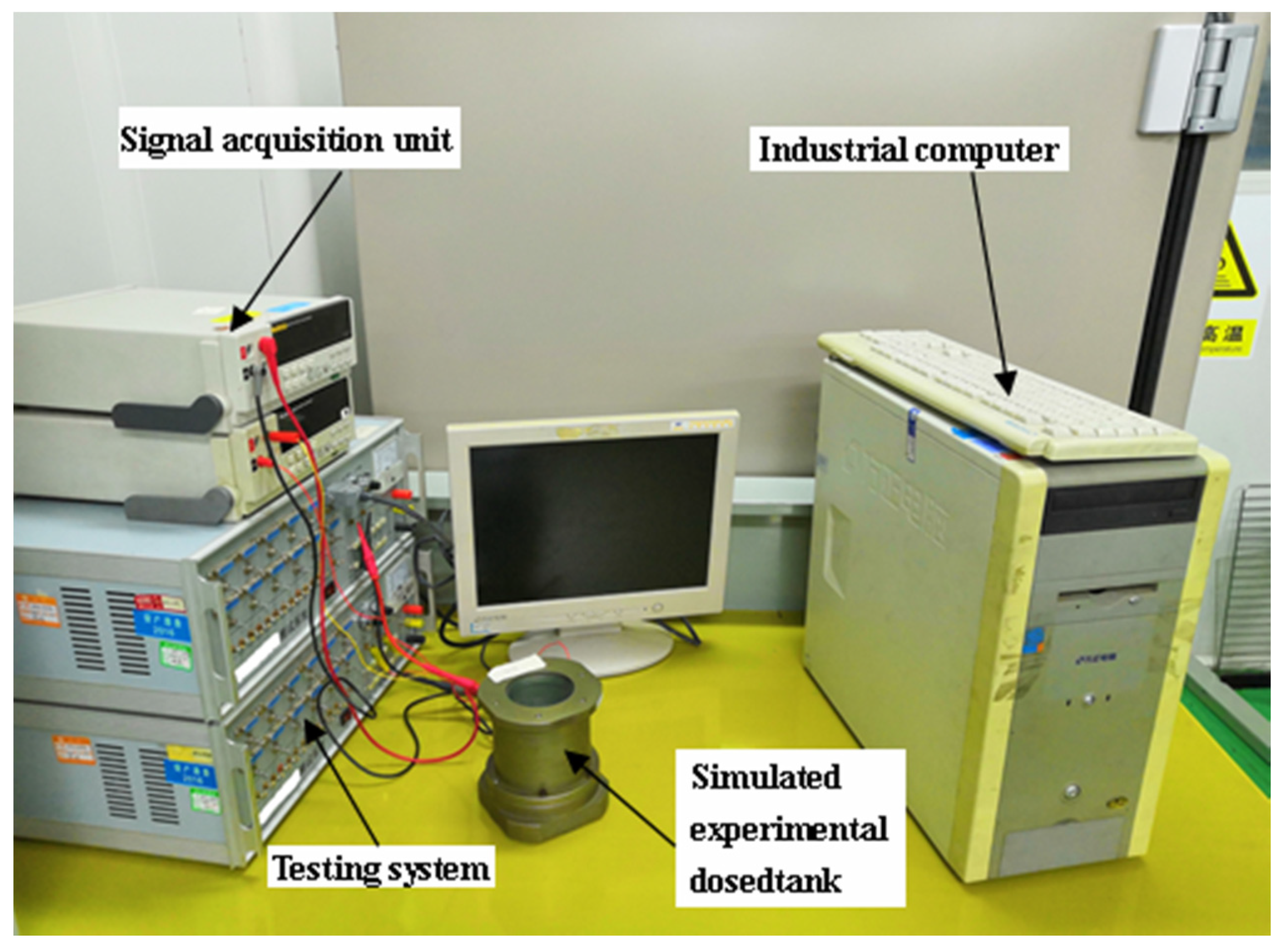
To verify the experimental methodologies, the gyro motor was tested on an experimental platform, from where we then conducted the data acquisition and time domain statistical feature extraction. The detailed acquisition method and procedures of the time domain statistical features are referred to in Soualhi et al. [37]. A photo of the experimental platform is shown in Figure 2.
In this study we carried out gyro motor fault signal acquisition on motor current signals to meet industrial needs. A gyro motor life span experiment needs to be done on a full life cycle basis without an accelerated test. The experiment utilized a newly assembled gyro motor whose bearing and other components had gone through strict testing before being assembled so that any defects are ruled out. In addition, in this study we put the experiment motor into a special test fixture and fastened the motor stator axis to prevent the experiment effect from being affected by any interference during the experiment. Simultaneously, motor degeneration is a gradual process and is not demanding in real time since the experimental data is in long-running tests, and it takes up a great deal of storage space. Consequently, timing data acquisition is employed to represent the state at a certain time interval.
Adjust the motor to ensure that it does not differ from a normal working gyro motor before the test begins. After the adjustment, re-fasten all motor fasteners to prevent interference from being introduced. The gyro motor’s rated voltage is 24 V and rated speed is 6000 rpm. The motor is placed inside a thermostatic lab to prevent temperature changes from exerting an influence on the experiment. Then, conduct bus data signal acquisition. The detailed acquisition method and procedures are as follows:
(1)
Place the cleaned bearing into the gyro motor to prevent interference from being introduced. Align the motor to a proper state and put the motor into a special test fixture.
(2)
Start the motor on a 24-h non-stop running mode with 24 h as a time unit.
(3)
Carry out one data acquisition in a fixed length way every 24 h of running. Acquire 10,000 points for each data set. Conduct the acquisition during the stable operation of the motor. If the motor needs to be restarted due to a power outage, then do not begin the data acquisition until the motor has run for five minutes.
(4)
Check the operational conditions of the gyro motor after every 24 h of operation, identify the state the gyro motor is in according to the changes in the gyro motor current and motor voice, see if the fault occurs, and keep records.
(5)
Restart the experiment by repeating steps (2) to (4) until the gyro motor loses efficacy when the test stops.

4.2. Time Domain Statistical Feature Analysis

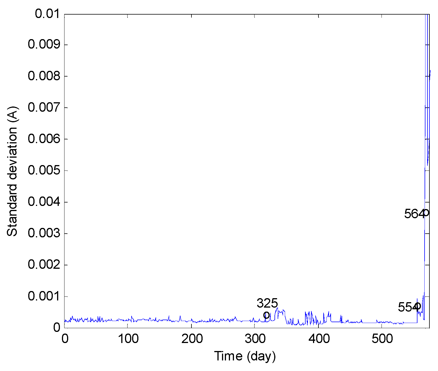
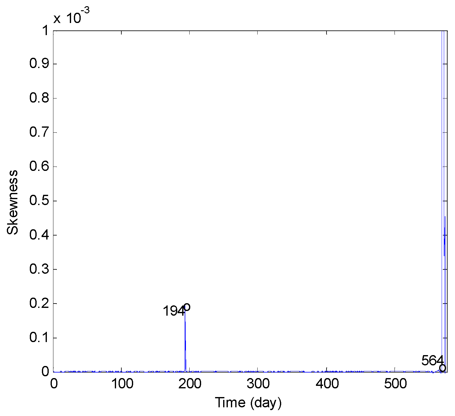
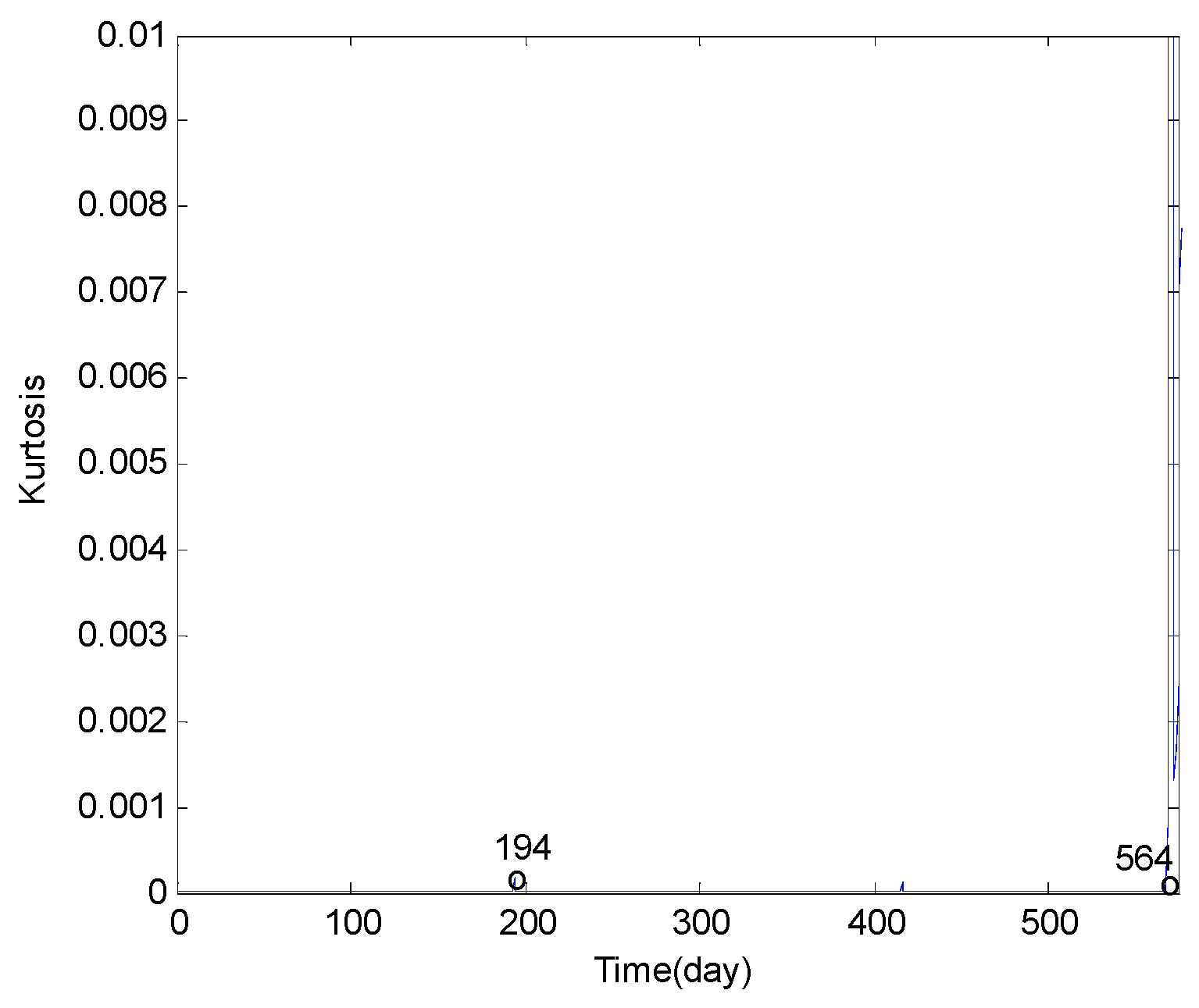
The whole gyro motor full life cycle experiment took 13,832 h. The signals were acquired from bus lines. A data set is acquired every 24 h and a total of 576 groups of data were acquired. The data included six common time domain statistical features. The motor lost its efficacy in the form of the outer ring, inner ring, and rolling body ware of varying degrees. Then, we analyzed the variation in the six time domain statistical features, as the mean value, standard deviation, crest factor, kurtosis, skewness, and power factor, as shown in Figure 3, Figure 4, Figure 5, Figure 6, Figure 7 and Figure 8.
Figure 3 presented the mean value of the gyro motor bus current. From the perspective of a full life cycle, the mean value of the current overall showed tendencies of gradual descend and gradual ascend. A wide oscillation diagram appeared when the efficacy started to be lost. Although Figure 3 is composed of the mean values of the current sample, to some extent it reflects the overall trend of the current. The current trend is explained from the perspective of energy. In the initial stage, the bearing was in a brand-new state and the initial error would lead to an increase in extra power. As the motor operated, components like bearing would become smoother due to break in. Under the same damping, the energy was less needed and the power decreased, so the current dropped. Subsequently, as the bearing increased, more and more energy was needed, and the current showed an upward trend. On Day 554, the mean value of the current exceeded and showed an upward trend, which, however, was close to the high point of the previous mean values. The actual motor experiment entered the degeneration state before failing and was judged from the traditional indicators and experience. On Day 564, the mean value showed drastic oscillation, indicative of faults in the motor, which resulted in instability in the current. The states prior to Day 554 were considered as a relatively healthy and stable.
However, in the actual test, the current sampling results still had many little fluctuations due to the test conditions and environment. On Day 215, the current showed an apparent upward trend. Current oscillation existed constantly for the following 100 days, which was inconsistent with the theoretical analysis. This was probably because after a day’s running, dust entered the motor bearing and caused micro-variation in the surface roughness and changes in the current, but not a failure. The following days, dust kept entering into the bearing and caused some degree of wear in the bearing, but this did not cause substantial damage rather than instability in the current. As the test continued, the wear would become smooth due to break-in and the value of the current would drop again and stabilize. This had a certain effect on the experiment but did not lead to failure. Meanwhile, some unpredictable factors impacted the experiment but did not cause damage. This was common in the engineering field. Therefore, all the same data were effective.
This study is viewed from the overall change in current and from the trend of a descend to ascend in shock failure; it was definite for fault state analysis. However, it was still difficult to analyze the state that was gradually getting close to failure, whereas such kind of state was the most useful for maintenance strategies. Therefore, the mean value of the current alone could not analyze well the health condition and the degeneration state that was getting close to failure.
Figure 4 is the standard deviation diagram of the gyro motor current. It shows that the standard deviation of the motor current was fairly stable prior to the first 325 days. This indicates that the value of the current acquired during the acquisition period deviated slightly from the mean value, an indicator of motor stability. Even though during the period from Day 215 to Day 325 some foreign matter might have entered into the bearing, the analysis revealed that it did not cause the bearing to fail, so there was no big fluctuation that deviated from the mean value during the acquisition period. This corroborated with what was showed in Figure 3. Starting from Day 325, the standard deviation showed some degree of fluctuation, indicating that following more than 300 days of running the current acquisition value deviated a great deal from the deviation value. On Day 554, the motor started to enter a degeneration state that was getting close to failure and there was greater fluctuation in the standard deviation. However, the fluctuation was not different from the fluctuation starting from Day 325, so the effect of the classification was ideal. Starting Day 564, the motor started to fail, and the standard deviation of the current began to fluctuate drastically for classification. This indicated that the standard deviation of the current alone could not analyze well the health conditions and the degeneration state that was getting close to failure.
Figure 5 and Figure 6 show that when in the stable state of a full life cycle, the skewness and kurtosis are close to the stable horizontal lines (humped) on Day 194. This was a disadvantage for classification and might be caused by interferences sensitive to the two indicators of skewness and kurtosis. Following Day 564, both indicators showed considerable improvement and there was no significant change on Day 554. The result presented suggest the two indicators only be employed when the faults appear. However, the changes during the process still caused interference and affected the diagnostic effect.
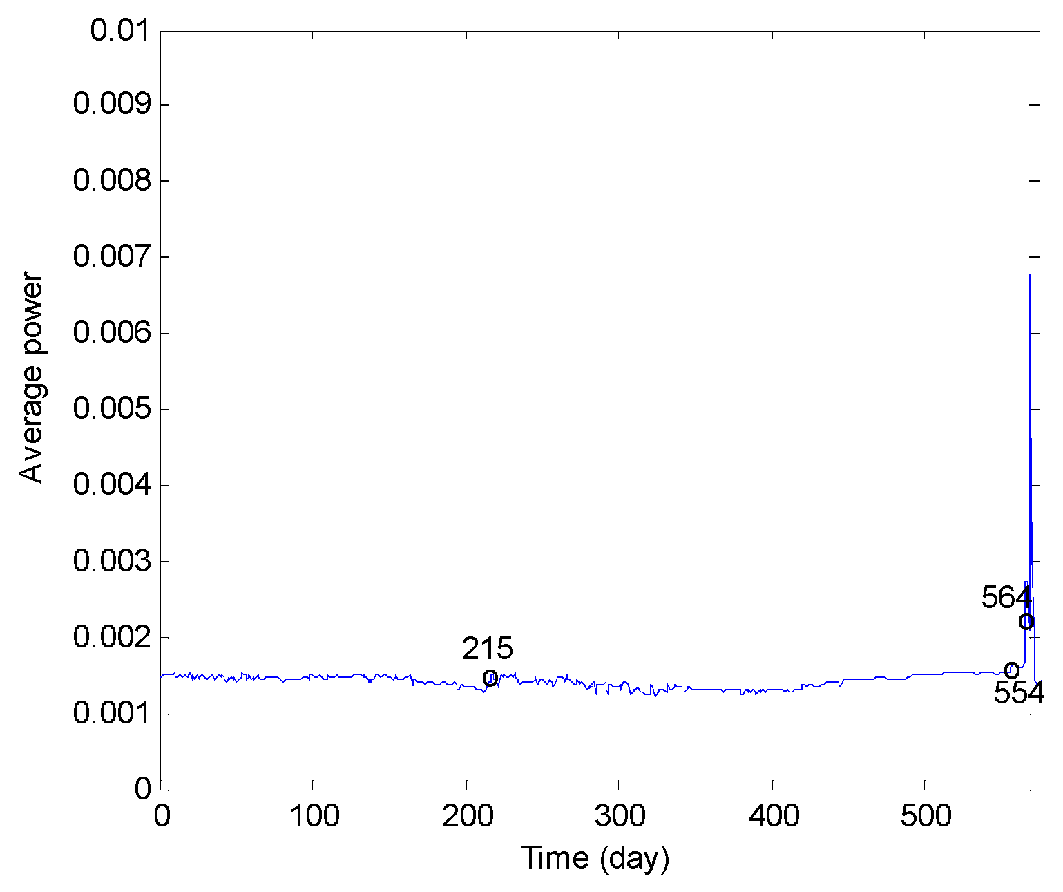
Figure 7 showed the power factor diagram of the gyro motor bus. From the perspective of a full life cycle, the power factor overall presented a gradual downward rather than upward trend, and a diagram of wide oscillation appeared when the efficacy was lost. This was generally consistent with the trend of the mean value of the current and the higher smoothness. On Day 554, the power factor exceeded the older values and showed a continual upward trend, but close to the previous high point, which was bad for classification. On Day 564, the power factor showed drastic oscillation, indicating that, as faults appeared on the motor, it caused the power factor to rise. On Day 215, the power factor showed a certain upward trend consistent with the current’s changed mean value. Therefore, the power factor alone could not provide an ideal analysis of the health conditions and the degeneration state that was getting close to failure.
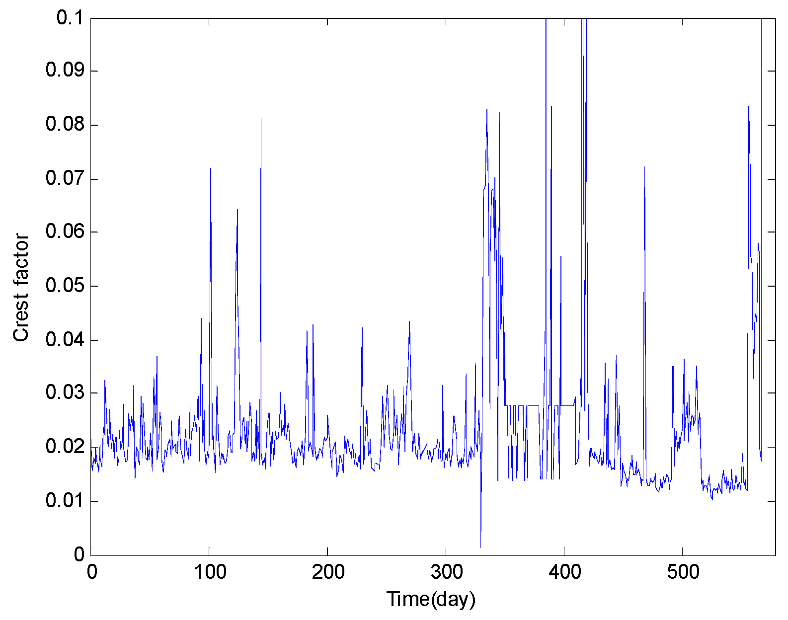
Figure 8 present the crest factor diagram and shows its insensitivity to the various states of the motor, which could not effectively reflect the gyro motor bearing’s stable state, the degeneration state before failure, nor the faulty state. Therefore, this indicator was not applicable to the analysis of gyro motor bearing states. The time domain statistical features are sorted out in Table 1.
Table 1 revealed that the time domain statistical indicators were utilized alone to analyze the various states of the gyro motor bearing’s full life cycle; the classification effects were relatively better only for the mean value, standard deviation, and power factor. However, the classification effects were not better for the other indicators, since the classification results of the degeneration states before the failure could not be delivered. Hence, using multi-statistical features for comprehensive classification is a more ideal option.

4.3. Experimental Results

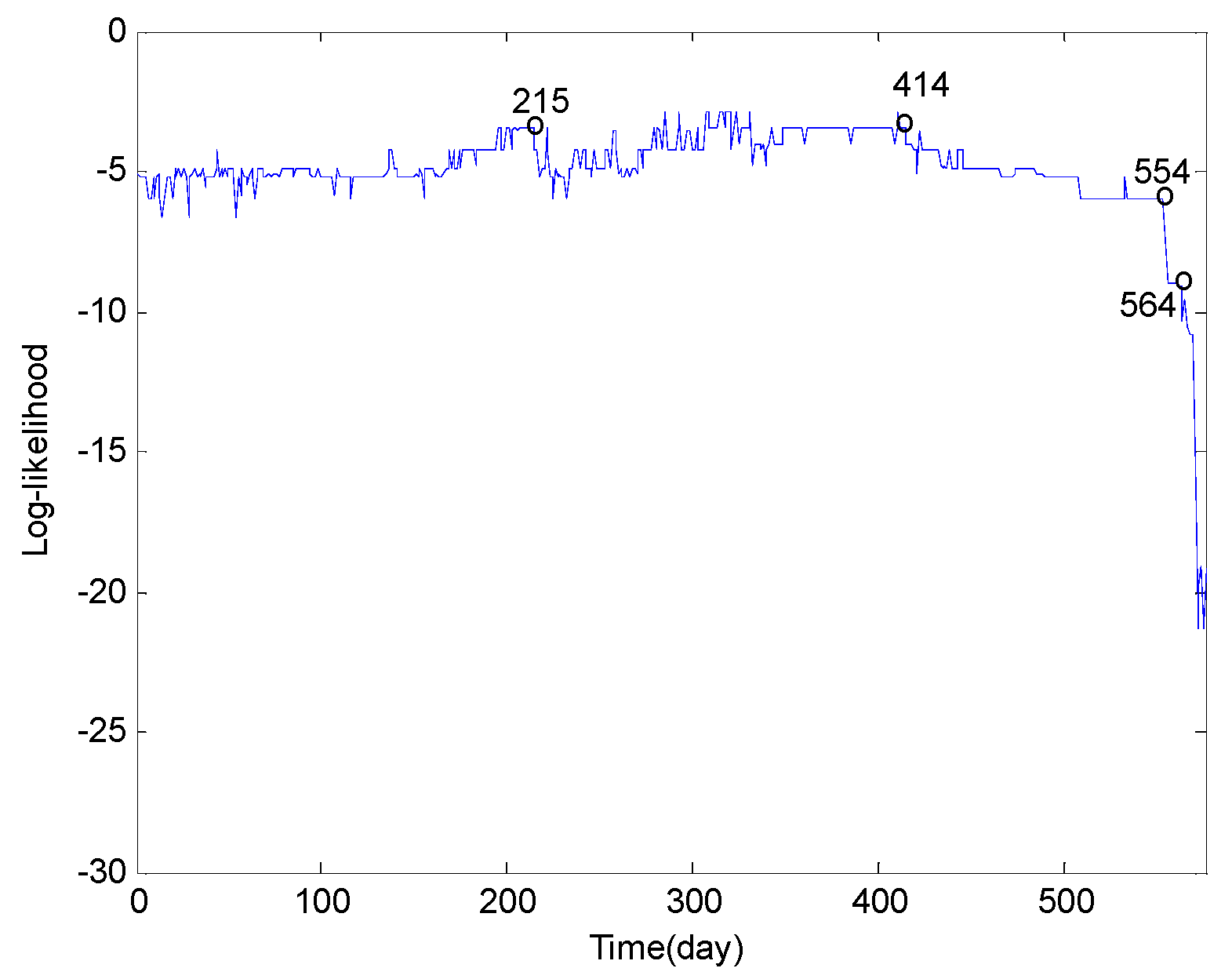
We performed feature reduction using the minimum intra-class distance algorithm on the 576 groups of time domain statistical features extracted from the gyro motor’s full life data over 576 days, and obtained three features: (1) the mean value; (2) standard deviation; and (3) power factor [41]. The three features were transformed into feature vectors to normalize the data extracted and we substituted the normalized data in the training HMM to obtain the full life cycle trained HMM. Following the normalization of the full life cycle data, we substituted the data into the full life cycle trained HMM in chronological order from the data that was extracted and obtained from the 576 log likelihood probabilities. If one takes time as the horizontal coordinates, and the log likelihood probability as the vertical coordinate, which had been obtained by substituting each day’s data in the HMM, you get the time-probability curve as shown in Figure 9.
The gyro motor has a running-in period about 60 days, as shown in Figure 9. In this period, because all kinds of parts were brand-new and needed to be run in, the curve showed more convex changes. From the curve, the time-probability curve of the motor also had a lot of oscillating changes in this period, with values ranging from −4.9 to −6.6. Because the running-in period of the gyro motor was at a routine experiment stage, only motors that had performed these experiments could perform the following. Therefore, the motor tested under the actual-use conditions would not be in this stage. From the 60th day to the 214th day, this was a steady run-in period. In this stage, the log likelihood probability value increased steadily and gradually, and the oscillation decreased, keeping the mean value between −3.4 and −6.0. From the average current graph in Figure 3, the current gradually decreased, which meant that, with the operation of the motor, the operation of each component was more stable. Between Day 215 and Day 414, the log likelihood probability oscillated around the maximum value, namely the normal stage, which also lasted the longest. Figure 3 showed the current in a relatively low steady stage and normal stage. Note that in this stage the full life cycle time-probability curve fluctuated for a while and the log likelihood probability oscillation decreased to −5.2 on Day 229 and the oscillation continued several times, returning to −3.4~−4.0.
Meanwhile, the current curve also had some oscillation. Changes in the current due to accidental factors would cause the statistical features extracted from the current to deviate from the normal value and the log likelihood probability to decline. This stage was also suggested from the consistencies of Figure 3 and Figure 9. Figure 9 showed that, between Day 414 and Day 553, the log likelihood probability gradually went down from −4.2 to −6.0, whereas Figure 3 indicated a gradually increasing value of the current, and the motor was actually in a state of degeneration. Figure 9 showed that, between Day 554 and Day 564, the log likelihood probability gradually went down from −8.9 to −9.0, whereas the value of the current in Figure 4 also reached a relatively high level that lasted only for 10 days before the oscillation started, indicative of the degeneration state before failure. After Day 564, the current vibrated drastically and Figure 9 showed that the log likelihood probability also went down rapidly. All generation stages of the life cycle are showed in Table 2.
Table 2 presented the actual situation and the running-in period impact is ignored. There are overlapping parts in the run-in period, normal state, and preliminary degeneration state. On the one hand, it is due to the influence of the accidental events, and on the other hand, it is also due to the gradual degradation process. The log likelihood probability of the degeneration state before failure and the failure state decreases significantly.
Hence, 15 groups of data were selected for verification in order to verify the time-probability curve. In these 15 groups of data, there were 5 states: the run-in period, normal state, preliminary degeneration state, degeneration state before failure, and failure state. Three days of data were randomly selected for each state, and it was used to verify the state estimation and life prediction. The specific results are shown in Table 3.
In Table 3, ①~⑤ represent the run-in period, normal state, preliminary degeneration state, degeneration state before failure, and failure state, respectively. Table 3 shows the 15 groups of data analysis. The diagnostic correctness rate is 100% during the degeneration state and degeneration state before failure. Of the nine groups of data from the run-in period, normal state, and preliminary degeneration state, seven groups were misjudged. This phenomenon occurs because the three states are close, and it also contains accidental events, all of which must overlap. If the run-in period, normal state, and preliminary degeneration state are defined as a healthy state, the curve can correctly classify all states to be divided like this in actual engineering. The estimation of the run-in state is the largest difference from the actual state for the estimation of the remaining life. This state is in the early stage of application and has less value for engineering applications. The estimation of the normal state, degeneration state before failure, and failure state are close to the actual state. The preliminary degeneration state is relatively close, too, and the normal state, preliminary degeneration state, and degeneration state before failure have the greatest value for the actual needs of the project, and can provide data reference for repair and replacement. These analyses can prove that the time-probability curve is accurate for relatively large stage estimates, and can also make better predictions of the life estimates for the normal state, preliminary degeneration state, and degeneration state before failure.
This analysis leads to present the following: (1) The overall test data curve and the curve of the current mean value went in the opposite directions and the pattern displayed provides evidence for the state wherein the test data was. (2) The longer the motor is in the normal state, the larger the log likelihood probability is obtained from the normal test data; otherwise, the smaller the log likelihood probability obtained from the normal test data. This indicated that the normal state took up the longest bearing life span and the normal log likelihood probability that was obtained from the test on normal data would be larger. The fault state variety and massive data acquisition that continues for the following faults due to the log likelihood probability obtained from test on fault data would be small. (3) New circumstances occurred due to a non-deviating normal state and reaching failure; instead, to continue for some time resulted from the log likelihood probability decreasing. The log likelihood probability increased a little when things got back to normal. This indicated that the method is reacting better to actual engineering accidents and if new situations arises this may cause some degree of overlap between the log likelihood probability of the preliminary degeneration state and of the normal state since it poses some difficulty to the matches. However, in actual engineering, the degeneration state before failure is the most important in ten days’ time and 240 h is enough to provide a buffer time for the maintenance strategies. (4) The evaluative method could judge the gyro motor degeneration processes fairly accurately. It could determine the temporal position the equipment was in, accomplishing the residual life prediction when the curve was ideal.

5. Comparing Analysis

A comparative analysis was performed using a multi-HMM state prediction method and a multi-HMM state prediction method to verify the effectiveness of the proposed prediction method.

5.1. Multi-HMM State Prediction Method

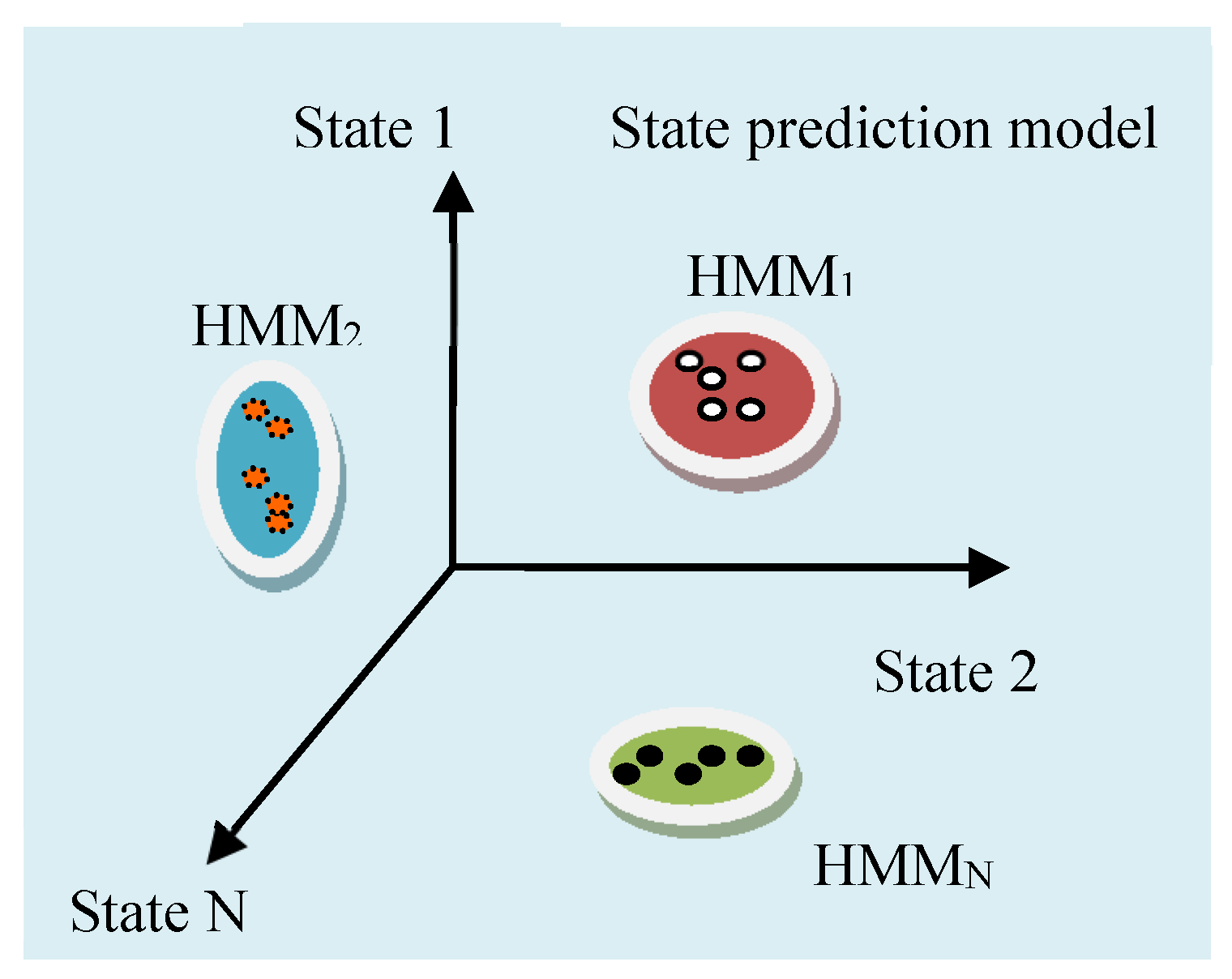
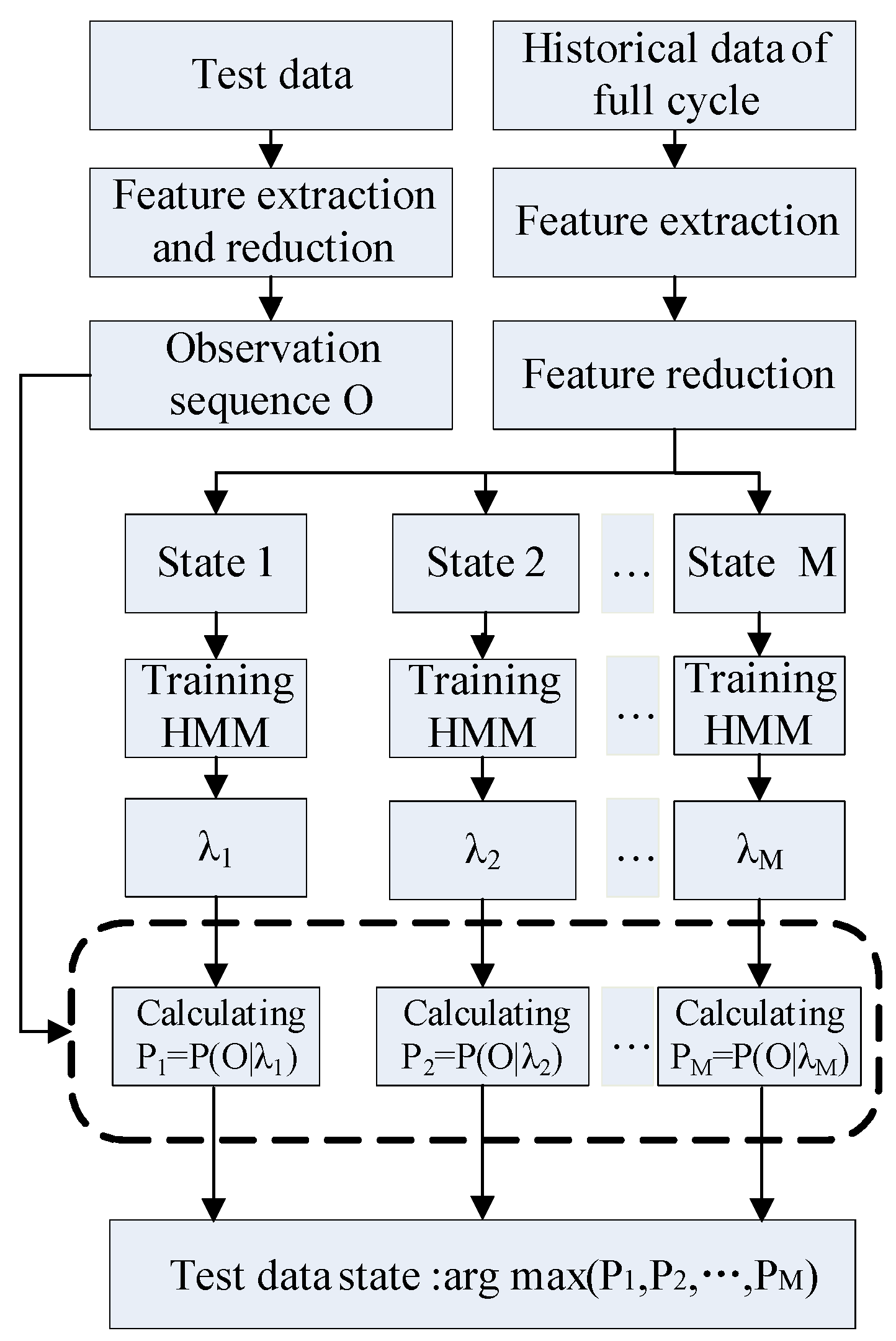
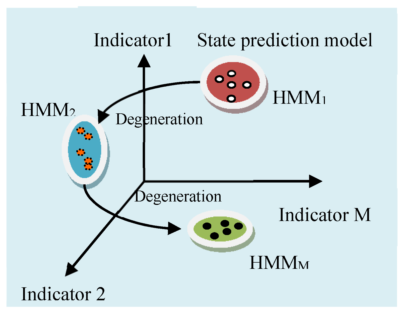
Using several HMM models as means of state prediction actually is to use trained the models to represent each type of degeneration state, substituting unknown state data into trained models to calculate the maximum log likelihood probability and thereby accomplishing fault state prediction. The structure is shown in Figure 10.
The flow chart of the multi-HMM fault prediction procedures are shown in Figure 11. The detailed steps are as follows: (1) Data acquisition: conduct training data acquisition on each state. (2) Feature extraction: normally, the signals acquired are not applied directly to the HMM’s diagnosis and prediction due to the original acquired signals containing a large amount of redundant information and noise and sometimes submerging the feature signals and causing fault classification errors. Hence, there is a need for feature extraction of the original data. (3) Feature reduction using all the features at the same time results in a large data size and low classification efficiency. This poses high demands on equipment hardware and real-time monitoring that cannot be achieved. Hence, there is a need for feature reduction. (4) State prediction: feature prediction is divided into two steps. The first step is to train the historical data and the second step is to classify the test data. For historical data, choose the feature signals of the most representative fault state to train and obtain the feature parameter λ.
Then, substitute the test data in Formula (1) to calculate the P ( O | λ ) probability. The correspondence maximum probability λM is the prediction result.

5.2. Health Condition HMM Prediction Method

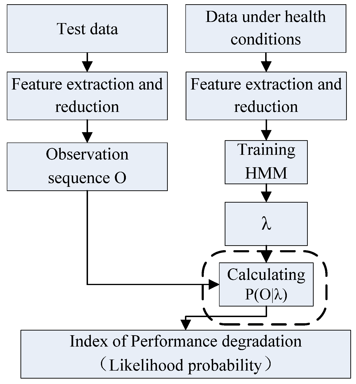
The gyro motor’s state degenerate from a healthy condition to failure, an irreversible process during the gyro motor state degeneration process. This study extracted data under healthy conditions during the state evaluation. The process carried out sample training on the data and then substituted test data to calculate the log likelihood probability, which actually reflects the membership grade of test data to the normal state. The larger the log likelihood probability is, the higher the possibility of a normal state membership for the test data; the smaller the log likelihood probability is, the higher the tendency of failure. The structure of the health condition an HMM prediction method is shown in Figure 12.
The flow chart of the health condition HMM prediction method is shown in Figure 13. The detailed procedures are the same as those of the multi-HMM state prediction method by setting up an alarm door threshold and to determine the degree of the test data’s deviation from the health condition and thereby accomplish the evaluation and prediction of the test state.
To sum up, during the gyro motor degeneration state diagnosis and evaluation, employing the two aforementioned methods faced the following problems. (1) When method one is used, the gyro motor full life cycle degenerates in the way of simultaneous failure of several components. Therefore, the eventual failure modes vary; hence, full data fault diagnosis and prediction cannot be described in one way and this adds difficulty to the HMM classification. (2) When method two is used, the part of the gyro motor state fault and evaluation that has the most industrial implications is evaluated as the state in which a gyro motor is in and the time until the faulty state. Using incomplete data for state evaluation actually reflects the similarity between the current and the normal state. Such a method does not take full advantage of prior knowledge. (3) Problems that both methods have: the gyro motor degeneration stages are generally classified by experience and each state requires a training HMM. If the length of each stage varies, the same data got different log likelihood probabilities and this affects the results of the evaluation and prediction.
Therefore, both the afore-discussed methods of gyro motor full life cycle state evaluation are inadequate. This study proposes a time-probability curve model in view of these inadequacies. The comparisons of the three methods are shown in Table 4.
Table 4 reveals that the time-probability curve model and the multi-HMM prediction method need the same amount of training data and have a higher data utilization ratio than the single HMM prediction method does. In terms of the prediction capability of residual life, the time-probability curve model is more accurate than the other two methods and does not need a degeneration state classification.

5.3. Test Analysis

In the test, the selection and division of the data remains the same as the division used in the prediction method of the life cycle time-probability curve. The training data is still used for training and the test data is still used for testing. The purpose is to enhance contrast. The experimental results are shown in Table 5.
In Table 5, ①~⑤ represent the run-in period, normal state, preliminary degeneration state, degeneration state before failure, and failure state. Table 5 shows the classification accuracy of the multi-HMM model state assessment method is 60%. The normal state and the degeneration state before failure have achieved completely correct predictions, while the run-in period, the preliminary degeneration state, and the failure state have lower correct rates. The characteristics of the normal state and degeneration state before failure are relatively clear, while the data in the run-in period and the preliminary degeneration state are relatively close, resulting in a miscalculation, especially in the form of various failure states, with large data changes, so it is easy to overflow. The multi-HMM model life estimation is related to the division of states, so in addition to the preliminary degeneration state and the failure state, the life estimation errors of the other three states are relatively large.
The output probability is estimated by using the state evaluation method of the health condition HMM prediction model, and the log likelihood probability obtained during the normal state and the preliminary degeneration state is basically the same as the time-probability curve. Since no degeneration data is used, the log likelihood probability of all the failure states is much smaller than −9.0; this method can determine the degree of state degradation by setting an alarm threshold, but it also cannot achieve a more accurate estimation of the remaining life.
Table 6 shows Table 3 with 5 comparisons to get the three prediction methods’ comparison results. The time-probability curve model has an accurate evaluation of the degeneration state before failure and failure state, especially for the estimation of residual life. For the health state, the running time of this stage is longer, and the experiment process contains accidental factors. The health state test data is prone to multi-point correspondence in the normal state, and it is difficult to judge the remaining life. In practical engineering applications, the normal state is not the focus of attention. The result has practical value to accurately predict and estimate the residual life in the degeneration state before failure. In the degeneration state before failure, the log likelihood probability curve presents a monotonic downward trend, and the log likelihood probability starts to be less than −6.0. In this stage, the log likelihood probability output from the state test data can have a more accurate corresponding relationship, which is used to estimate the remaining life.

6. Discussion

The traditional HMM is a rather mature mathematical model, which after being trained can diagnose and predict the state of the test data by means of the log likelihood probability of the output [37,42,43]. The data membership of the training model is correlated with the training data besides from the data itself; that is, the model first conducts classification according to data similarity. When the similarity matches, the amount of data in the same class can influence the size of the log likelihood probability and could provide a basis for the classification. Based on this trait, aside from the classification of the test data, all training data are substituted in the original training model to generate a time-probability curve, which is compared with the log likelihood probability of the test data output that can accomplish an accurate classification and prediction. This is the core idea of the proposed model. Nevertheless, using the HMM structure, the proposed model needs development and provides a new perspective to the application.
The proposed model is a development improvement for the HMM. This model combined the influence of the amount of training data on the prediction results while making use of the full advantage of the HMM structure. The amount of training data would directly affect the log likelihood probability obtained when the test data and training data share the same similarity. This is equivalent to a classification of prediction data, making the time-probability curve show chronological variation. The model that was proposed by this study has a better state evaluation and prediction ability when the data showed monotonous variation tendency. This stage is more likely to appear in the gyro motor’s later degeneration state and the model is better for gyro motor state diagnosis and prediction. Moreover, this model could directly match the positions where the degeneration states have no detailed classification. The classification method employed was analyzed with the convenience of expression.
In addition to solving the problem of gyro motor state evaluation and prediction, the method employed has another advantage—a certain degree of fault tolerance for accidental incidents. This study analyzed the accidental incidents that were affected by the normal classification results due to the full life cycle data. Although accidental incidents would cause some overlap with the degeneration states, which increased the difficulty of the evaluation and prediction, in practical engineering applications, the influence of the health conditions and preliminary degeneration states was not significant on equipment maintenance and replacement strategies, whereas evaluation and prediction of the stage from a later degeneration state to a failure state is the most important. The model was showed to be most sensitive to the later degeneration state and failure state, indicating the advantage of the proposed method. The prediction proposed method provided the reference for the diagnosis and prediction of other equipment, becoming a powerful tool for state diagnosis and prediction.
In the gyro motor state prediction field, signal acquisition is only done by non-invasive ways, and model training and calculation by means of time domain statistical features in the special work environment. The proposed model makes full use of the HMM’s strength, which when combined with the features of a gyro motor can accomplish state prediction within the full life cycle scope. This model is applied to fields such as fault diagnosis, speech, and image recognition. When the amounts of same-class data are the same, the model is an ordinary HMM, whereas when the amounts vary, the model can provide fairly accurate classification and prediction. In practical engineering applications, generally the amounts of same-class data acquired according to certain rules varies, or under the conditions when the results are not affected, human intervention is imposed to add or reduce the amounts of same-class data. The proposed model has gained a wider application scope and provides a powerful prediction tool for various practical fields.

7. Conclusions

This study proposes a time-probability curve model for a gyro motor full life cycle prediction. The results indicate that the full life cycle time-probability curve based on the HMM displayed different curve features in different degeneration states and reflected the accurate changes in the process of the gyro motor’s states. The results were also verified by means of a current mean value curve, indicating that the model could deliver accurate gyro motor state evaluation and prediction. The model provides a better approach to gyro motor state evaluation and prediction, and it is beneficial to the improvement of mechanical gyroscope and inertia system reliability. In addition, this method extends its scope to industrial applications, providing a powerful tool for state diagnosis and prediction for different equipment. Due to time limits, the experimental conditions, and energy, this model still needs improvement in the following aspects: (1) a future study is needed for the matching method that is employed by the time–probability curve to conduct evaluation and prediction. The goal is to carry out real-time diagnosis and prediction via full life cycle data. This facilitates online measuring and expands the application scope. (2) The prediction results are not only correlated to the similarity of the tested states but also to the amount of training samples acquired for each state. The amounts of historical data for each state are the same or closer under the real condition when the test data and training data share the same similarities and the different degrees of the time–probability curve drops significantly.

Author Contributions

Conceptualization, L.D.; Data curation, B.M.; Formal analysis, Z.Y.; Writing—original draft, L.D. and J.W.; Writing—review & editing, M.-L.T. and L.-L.L. All the authors contributed equally to the conception of the idea, implementing and analyzing the experimental results, and writing the manuscript. All authors have read and agreed to the published version of the manuscript.

Funding

This work was funded by the National Natural Science Foundation of China [Project No. 51475136].

Conflicts of Interest

The authors declare no conflict of interest.

References

  1. Darong, H.; Lanyan, K.; Chu, X.; Zhao, L.; Mi, B. Fault diagnosis for the motor drive system of urban transit based on improved Hidden Markov Model. Microelectron. Reliab. 2018, 82, 179–189. [Google Scholar] [CrossRef]
  2. Tobon-Mejia, D.A.; Medjaher, K.; Zerhouni, N.; Tripot, G. A data-driven failure prognostics method based on mixture of Gaussians hidden Markov models. IEEE Trans. Reliab. 2012, 61, 491–503. [Google Scholar] [CrossRef] [Green Version]
  3. Zhu, J.; Ge, Z.; Song, Z. HMM-driven robust probabilistic principal component analyzer for dynamic process fault classification. IEEE Trans. Ind. Electron. 2015, 62, 3814–3821. [Google Scholar] [CrossRef]
  4. Zhang, S.-q.; Lin, K.-P. Short-term traffic flow forecasting based on data-driven model. Mathematics 2020, 8, 152. [Google Scholar] [CrossRef] [Green Version]
  5. Dash, S.; Venkatasubramanian, V. Challenges in the industrial applications of fault diagnostic systems. Comput. Chem. Eng. 2000, 24, 785–791. [Google Scholar] [CrossRef]
  6. Venkatasubramanian, V.; Rengaswamy, R.; Kavuri, S.N.; Yin, K. A review of process fault detection and diagnosis: Part III: Process history based methods. Comput. Chem. Eng. 2003, 27, 327–346. [Google Scholar] [CrossRef]
  7. Rabiner, L.R. A tutorial on hidden Markov models and selected applications in speech recognition. Proc. IEEE 1989, 77, 257–286. [Google Scholar] [CrossRef]
  8. Wang, S.; Xiang, J.; Zhong, Y.; Zhou, Y. Convolutional neural network-based hidden Markov models for rolling element bearing fault identification. Knowl. Based Syst. 2018, 144, 65–76. [Google Scholar] [CrossRef]
  9. Baruah, P.; Chinnam, R.B. HMMs for diagnostics and prognostics in machining processes. Int. J. Prod. Res. 2005, 43, 1275–1293. [Google Scholar] [CrossRef]
  10. Ilhem, B.; Amar, B.; Lebaroud, A. Classification method for faults diagnosis in reluctance motors using Hidden Markov Models. In Proceedings of the Industrial Electronics (ISIE), 2014 IEEE 23rd International Symposium on IEEE, Istanbul, Turkey, 1–4 June 2014; pp. 984–991. [Google Scholar]
  11. Le, D.; Provost, E.M. Emotion recognition from spontaneous speech using hidden Markov models with deep belief networks. In Proceedings of the 2013 IEEE Workshop on Automatic Speech Recognition and Understanding (ASRU), Olomouc, Czech Republic, 8–12 December 2013; pp. 216–221. [Google Scholar]
  12. Cai, Y.; Shi, X.; Shao, H.; Wang, R.; Liao, S. Energy efficiency state identification in milling processes based on information reasoning and Hidden Markov Model. J. Clean. Prod. 2018, 193, 397–413. [Google Scholar] [CrossRef]
  13. Putland, R.L.; Ranjard, L.; Constantine, R.; Radford, C.A. A hidden Markov model approach to indicate Bryde’s whale acoustics. Ecol. Indic. 2018, 84, 479–487. [Google Scholar] [CrossRef]
  14. Roman-Galvez, R.; Roman-Roldana, R.; Martınez-Arozab, J.; Gomez-Loper, J.F. Semi-hidden Markov models for generation and analysis of sequences. Math. Comput. Simul. 2015, 118, 320–328. [Google Scholar] [CrossRef]
  15. Ali, S.M.; Bhatti, U.I.; Munawwar, K.; Alsaggaf, U.M.; Mansoor, S.; Ali, J. Gyroscopic Drift Compensation by Using Low Cost Sensors for Improved Attitude Determination. Measurement 2018, 116, 199–206. [Google Scholar] [CrossRef]
  16. Jang, H.S.; Bae, K.Y.; Park, H.S.; Sung, D.K. Solar power prediction based on satellite images and support vector machine. IEEE Trans. Sustain. Energy 2016, 7, 1255–1263. [Google Scholar] [CrossRef]
  17. Wang, S.; Chen, M.; Song, M. Energy constraints, green technological progress, and business profit ratios: Evidence from big data of Chinese enterprises. Int. J. Prod. Res. 2018, 56. [Google Scholar] [CrossRef]
  18. Zhang, W.; Liu, K.; Zhang, W.; Zhang, Y.; Gu, J. Deep Neural Networks for wireless localization in indoor and outdoor environments. Neurocomputing 2016, 194, 279–287. [Google Scholar] [CrossRef]
  19. Ren, Y.; Li, H.; Lin, H.C. Optimization of Feedforward Neural Networks Using an Improved Flower Pollination Algorithm for Short-Term Wind Speed Prediction. Energies 2019, 12, 4126. [Google Scholar] [CrossRef] [Green Version]
  20. Paya, B.A.; Esat, I.I.; Badi, M.N.M. Artificial neural network based fault diagnostics of rotating machinery using wavelet transforms as a preprocessor. Mech. Syst. Signal Process. 1997, 11, 751–765. [Google Scholar] [CrossRef]
  21. Li, B.; Chow, M.Y.; Tipsuwan, Y.; Hung, J.C. Neural-network-based motor rolling bearing fault diagnosis. IEEE Trans. Ind. Electron. 2000, 47, 1060–1069. [Google Scholar] [CrossRef] [Green Version]
  22. Gan, S.; Liang, S.; Li, K.; Deng, J.; Cheng, T. Trajectory length prediction for intelligent traffic signaling: A data-driven approach. IEEE Trans. Intell. Transp. Syst. 2018, 19, 426–435. [Google Scholar] [CrossRef]
  23. Nagulan, S.; Selvaraj, J.; Arunachalam, A.; Sivanandam, K. Performance of artificial neural network in prediction of heave displacement for non-buoyant type wave energy converter. IET Renew. Power Gener. 2016, 11, 81–84. [Google Scholar] [CrossRef]
  24. Zhang, L.; Xiong, G.; Liu, H.; Zou, H.; Guo, W. Applying improved multi-scale entropy and support vector machines for bearing health condition identification. Proc. Inst. Mech. Eng. Part C J. Mech. Eng. Sci. 2010, 224, 1315–1325. [Google Scholar] [CrossRef]
  25. Widodo, A.; Kim, E.Y.; Son, J.D.; Yang, B.S.; Tan, A.C.; Gu, D.S.; Choi, B.-K.; Mathew, J. Fault diagnosis of low speed bearing based on relevance vector machine and support vector machine. Expert Syst. Appl. 2009, 36, 7252–7261. [Google Scholar] [CrossRef]
  26. Widodo, A.; Yang, B.S.; Han, T. Combination of independent component analysis and support vector machines for intelligent faults diagnosis of induction motors. Expert Syst. Appl. 2007, 32, 299–312. [Google Scholar] [CrossRef]
  27. Rojas, A.; Nandi, A.K. Practical scheme for fast detection and classification of rolling-element bearing faults using support vector machines. Mech. Syst. Signal Process. 2006, 20, 1523–1536. [Google Scholar] [CrossRef]
  28. Li, L.; Lv, C.M.; Tseng, M.L.; Song, M. Renewable energy utilization method: A novel Insulated Gate Bipolar Transistor switching losses prediction model. J. Clean. Prod. 2018, 176, 852–863. [Google Scholar] [CrossRef]
  29. Li, L.; Lin, G.Q.; Tseng, M.L.; Tan, K.; Lim, M.K. A Maximum Power Point Tracking Method for PV System with Improved Gravitational Search Algorithm. Appl. Soft Comput. 2018, 65, 333–348. [Google Scholar] [CrossRef]
  30. Zhang, F.; Zhang, Z.; Zhang, P.; Wang, S. UD-HMM: An unsupervised method for shilling attack detection based on hidden Markov model and hierarchical clustering. Knowl. Based Syst. 2018, 148, 146–166. [Google Scholar] [CrossRef]
  31. Liang, J.; Ma, M.; Sadiq, M.; Yeung, K.H. A filter model for intrusion detection system in Vehicle Ad Hoc Networks: A hidden Markov methodology. Knowl. Based Syst. 2019, 163, 611–623. [Google Scholar] [CrossRef]
  32. Fu, R.; Wang, H.; Zhao, W. Dynamic driver fatigue detection using hidden Markov model in real driving condition. Expert Syst. Appl. 2016, 63, 397–411. [Google Scholar] [CrossRef]
  33. Khan, S.S.; Karg, M.; Kuli, D.; Hoey, J. Detecting falls with X-Factor Hidden Markov Models. Appl. Soft Comput. 2017, 55, 168–177. [Google Scholar] [CrossRef] [Green Version]
  34. Yuwono, M.; Guo, Y.; Wall, J.; Li, J.; West, S.; Platt, G.; Su, S.W. Unsupervised feature selection using swarm intelligence and consensus clustering for automatic fault detection and diagnosis in Heating Ventilation and Air Conditioning systems. Appl. Soft Comput. 2015, 34, 402–425. [Google Scholar] [CrossRef]
  35. Song, M.; Wang, J.; Zhao, J.; Baležentis, T.; Shen, Z. Production and safety efficiency evaluation in Chinese coal mines: Accident deaths as undesirable output. Ann. Oper. Res. 2018, 291, 827–845. [Google Scholar] [CrossRef]
  36. Song, M.; Du, Q. Analysis and exploration of damage-reduction measures for flood disasters in China. Ann. Oper. Res. 2019, 283, 795–810. [Google Scholar] [CrossRef]
  37. Song, M.; Wang, S. The impact of knowledge trade on sustainable development and environment-biased technical progress. Technol. Forecast. Soc. Chang. 2019, 144, 512–523. [Google Scholar] [CrossRef]
  38. Xiong, X.; Chen, L.; Liang, J. A new framework of vehicle collision prediction by combining SVM and HMM. IEEE Trans. Intell. Transp. Syst. 2018, 19, 699–710. [Google Scholar] [CrossRef]
  39. Soualhi, A.; Clerc, G.; Razik, H.; Guillet, F. Hidden Markov models for the prediction of impending faults. IEEE Trans. Ind. Electron. 2016, 63, 3271–3281. [Google Scholar] [CrossRef]
  40. Tobon-Mejia, D.A.; Medjaher, K.; Zerhouni, N.; Tripot, G. Hidden Markov models for failure diagnostic and prognostic. In Proceedings of the Prognostics and System Health Management Conference (PHM-Shenzhen), Shenzhen, China, 24–25 May 2011; pp. 1–8. [Google Scholar]
  41. Dong, L.; Li, W.M.; Wang, C.H.; Lin, K.P. Gyro motor fault classification model based on a coupled hidden Markov model with a minimum intra-class distance algorithm. Proc. Inst. Mech. Eng. Part I J. Syst. Control Eng. 2019, 234. [Google Scholar] [CrossRef]
  42. Soualhi, A.; Razik, H.; Clerc, G.; Doan, D.D. Prognosis of bearing failures using hidden Markov models and the adaptive neuro-fuzzy inference system. IEEE Trans. Ind. Electron. 2014, 61, 2864–2874. [Google Scholar] [CrossRef]
  43. Campos-Delgado, D.U.; Pecina-Sánchez, J.A.; Espinoza-Trejo, D.R.; Arce-Santana, E.R. Diagnosis of open-switch faults in variable speed drives by stator current analysis and pattern recognition. IET Electr. Power Appl. 2013, 7, 509–522. [Google Scholar] [CrossRef]
Figure 1. The flow chart of the state prediction based on the hidden Markov model (HMM).
Symmetry 12 01750 g001
Figure 2. A view of the gyro motor test system.
Symmetry 12 01750 g002
Figure 3. Mean value change chart of the current signal.
Symmetry 12 01750 g003
Figure 4. Standard deviation diagram of the current signal.
Symmetry 12 01750 g004
Figure 5. Skewness diagram of the current signal.
Symmetry 12 01750 g005
Figure 6. Kurtosis diagram of the current signal.
Symmetry 12 01750 g006
Figure 7. Average power diagram of the current signal.
Symmetry 12 01750 g007
Figure 8. Crest factor diagram of the current signal.
Symmetry 12 01750 g008
Figure 9. Full life cycle time-probability curve of the gyro motor.
Symmetry 12 01750 g009
Figure 10. The fault prediction structure of the multi-HMM model.
Symmetry 12 01750 g010
Figure 11. Flow chart of fault prediction for the multi- HMM model.
Symmetry 12 01750 g011
Figure 12. Structure diagram of fault prediction for the single HMM model.
Symmetry 12 01750 g012
Figure 13. Flow chart of the fault prediction for a single HMM model.
Symmetry 12 01750 g013
Table 1. Life cycle characteristic comparison of the common time domain statistical features.
StateChange TendencyClassification EffectDegeneration State Indication before Failure
Name
Mean value averageobvious
Standard deviation averageobvious
Kurtosis fairly badnot obvious
Skewness fairly badnot obvious
Crest factorRepeated oscillationvery badnot obvious
Power factor averageobvious
Note: stands for down; for up and for stable; for basically invariant.
Table 2. Probability range for all the degenerate stages of the life cycle.
StateRunning-In PeriodRun-In PeriodNormal StatePreliminary Degeneration StateDegeneration State before FailureFailure State
Content
Working days
(day)
601544141191012
Log likelihood
probability range
−4.9~−6.6−3.4~−6.0−5.1~−3.4−4.2~−6.0−8.9~−9.0<−9.0
Table 3. Test data of the time-probability curve in the life cycle.
Select SamplesActual StateProbabilityState EstimationActual Remaining Life (day)Remaining Life Prediction
(day)
Day 72 −5.1①, ② or ③491>63
Day 79−4.9①, ② or ③484>68
Day 171−4.1①, ② or ③392>140
Day 208−3.4355149~368
Day 314−2.8249233~256
Day 385−4.1①, ② or ③178>140
Day 443−4.2①, ② or ③120>140
Day 468−5.2①, ② or ③95>55
Day 516−6.0① or ③4710~54
Day 555−8.982~9
Day 557−8.962~9
Day 562−9.012~9
Day 564−15.500
Day 568−21.300
Day 570−10.300
Table 4. Comparison of three methods of evaluation and prediction based on the HMM model.
StateMulti-HMM Prediction MethodSingle HMM Prediction MethodTime-Probability Curve Model
Content
Data needed to be trainedFull life cycle dataData under health conditionsFull life cycle data
Utilization ratio of training dataHighLowHigh
Evaluation methodState identification by means of output probabilityState identification by means of alarm doorState identification by means of time-probability curve
Life span prediction capabilityEstimation stageEstimation stageFairly accurate
Classification of degeneration stateNeededNot neededNot needed
Table 5. Test data of the life cycle multi-HMM state prediction method and health condition HMM prediction method.
Select SamplesActual StateResidual LifeMulti-HMM State Prediction MethodHealth Condition HMM Prediction Method
Classification ResultsRemaining Life Prediction
(day)
Log Likelihood ProbabilityRemaining Life Prediction
(day)
Day 72491Error>10−5.0Unattainable
Day 79484Right>349−4.9
Day 171392Error>149−4.2
Day 208355Right>149−3.4
Day 314249Right>149−2.8
Day 385178Right>149−4.0
Day 443120Error>149−4.2
Day 46895Error>10−5.2
Day 51647Right>10−6.0
Day 5558Right0~9−9.1
Day 5576Right0~9−9.1
Day 5621Right0~9−9.2
Day 5640Right0-Inf(overflow)
Day 5680-Inf(overflow)0-Inf(overflow)
Day 5700-Inf(overflow)0-Inf(overflow)
Table 6. The experimental result comparison of the three models’ evaluation and prediction methods.
Comparative ContentMulti-HMM State Prediction MethodHealth Condition HMM Prediction MethodTime-Probability Curve Model
Assessment resultsOutput classification resultsOutput log likelihood probabilityJudging the state by time-probability curve
Residual life estimationLarger errorInestimableHigh accuracy
Dependence on partitioned StatesNeededNot neededNot needed
Publisher’s Note: MDPI stays neutral with regard to jurisdictional claims in published maps and institutional affiliations.